


1. Introduction
It is well known that waves become attenuated as they propagate through an inhomogeneous disordered medium that has randomly varying properties. The term ‘localisation’ is used to describe this phenomenon since the waves are localised in space. Localisation is recognised as a multiple scattering effect caused by incoherent reflections from within the disordered medium and is an energy-conserving process; that is, attenuation is not a feature of natural physical dissipative effects.
The pioneering work of Anderson (Reference Anderson1958) which first described localisation in quantum systems has since been applied to many other physical systems supporting wave motion. Amongst these, considerable attention has been paid to the propagation of water waves over randomly varying bathymetry and this is the main initial focus of this paper. Early work in this area considered the randomness be manifested by rectangular steps in the bed. Following the experiments of Belzons, Guazzelli & Parodi (Reference Belzons, Guazzelli and Parodi1988), Devillard, Dunlop & Souillard (Reference Devillard, Dunlop and Souillard1988) used both shallow water and wide-spacing analogous full linear potential theory to consider the effect of random stepped bathymetry on wave propagation. Their numerical results supported an asymptotic theory based on a long-wavelength assumption that attenuation (the spatial rate of decay and the reciprocal of localisation length) is proportional to the square of the wave frequency. For longer waves, their numerical results based on shallow-water theory diverged, unsurprisingly, from the asymptotic long-wavelength theory and from numerical simulations based on full potential theory, and indicated that attenuation tended to a constant for high frequencies. Full linear potential theory suggested otherwise: that attenuation becomes exponentially weak as wavelengths tend towards the short-wavelength regime and this was explained as being associated with the exponential decay of wave energy throughout the fluid depth.
Other work on random beds worthy of note include a series of papers by Nachbin and coauthors (see Nachbin & Papanicolaou Reference Nachbin and Papanicolaou1992a,Reference Nachbin and Papanicolaoub; Nachbin Reference Nachbin1995). Much of the work on waves over random beds have supported the findings outlined previously. Within a linearised setting Mei, Stiassnie & Yue (Reference Mei, Stiassnie and Yue2005, § 7.4) applies a multiple-scale method (based on the work of Kawahara et al. Reference Kawahara, Yoshimura, Nakagawa and Ohsaka1976) for non-shallow potential flow and reaches similar conclusions. The calculation results in an explicit formula for the attenuation rate which is linked to the assumed statistical properties of the bed (now assumed to be defined by a smoothly varying function), as well as wavelength and the mean water depth. Around the same time, a number of papers (see Pihl et al. Reference Pihl, Jørgen, Mei and Hancock2002; Grataloup & Mei Reference Grataloup and Mei2003; Mei & Li Reference Mei and Li2004) applied similar multiple-scale analysis to various nonlinear descriptions of wave propagation. In particular, Mei & Li (Reference Mei and Li2004) and Grataloup & Mei (Reference Grataloup and Mei2003) considered weakly nonlinear long-wavelength theories (Boussinesq approximations). The analytically derived formulae for wave attenuation differed in that they predicted attenuation increasing like the frequency squared across all frequencies. Thus, there is no levelling off in the attenuation as described by Devillard et al. (Reference Devillard, Dunlop and Souillard1988) nor exponential decay as predicted by full linear potential theory.
More recently, Bennetts, Peter & Chung (Reference Bennetts, Peter and Chung2015) returned to the problem of linear full potential theory and performed a series of careful numerical simulations, over stepped beds, which they compared with the theory described by Mei et al. (Reference Mei, Stiassnie and Yue2005, § 7.4). They estimated the attenuation of individual waves, averaged over different realisations of random bathymetry and showed attenuation is significantly weaker than predicted by the theory. They correctly conclude that the ensemble averaging process used in the multiple-scale analysis contributes to an over-prediction of the decay of wave energy due to phase cancellation of propagating waves. Bennetts et al. (Reference Bennetts, Peter and Chung2015) also attempted to correct for the failings of the existing modelling by including both left- and right-going waves in the leading-order solution and by assuming a dependence on the random variables (i.e. stochastic) in the leading-order solution, as opposed to making the usual assumption that it is deterministic.
In this paper we revisit the problem of scattering by random bathymetry using a long-wavelength/shallow-water model which reduces the scattering process to solving an ordinary differential equation (ODE) that includes a coefficient of a random variable with given statistical properties (see § 3). In particular, the random variations in height are considered small compared with the depth. Our analysis (§ 4) is different to previous approaches. First, we assume the randomness occupies a semi-infinite region and define the problem in terms of an incident wave which has the effect of introducing an energy budget. Like Bennetts et al. (Reference Bennetts, Peter and Chung2015) we include left- and right-propagating waves, but we assume the leading-order solution is deterministic. Like Mei et al. (Reference Mei, Stiassnie and Yue2005, § 7.4) (and others) we adopt a multiple-scale approach, but note that the ensemble averaging which determines the attenuation requires careful consideration to remove phase cancellations which are not associated with multiple scattering. In making this correction we also show that energy is conserved.
Theory is compared with numerical simulations which are described in § 5 of the paper. In § 6 we use an extension of the model (derived in the Appendix) which allows for the surface of the water to be entirely covered by fragmented ice of variable thickness. The ODE that results differs from the variable bathymetry case only in the definition of three scaling coefficients and a dispersion relation; theory and numerical results are compared in § 7.
There are a number of existing studies in the literature that have explored the relationship between attenuation as a result of multiple scattering through randomness in ice. Only a few are three dimensional (e.g. Bennetts et al. Reference Bennetts, Peter, Squire and Meylan2010; Montiel, Squire & Bennetts Reference Montiel, Squire and Bennetts2016) and most make the same two-dimensional simplification made here. Others such as Mosig, Montiel & Squire (Reference Mosig, Montiel and Squire2019) have derived one-dimensional models in the form of a transport equation derived from the work of Ryzhik, Papanicolaou & Keller (Reference Ryzhik, Papanicolaou and Keller1996) investigating elastic waves in random media. Attenuation due to changes in the thickness of ice were considered by Kohout & Meylan (Reference Kohout and Meylan2008) who represent ice floes as a series of thin elastic plates with free edges floating in the surface with zero (non-Archimedian) draught. Additional dissipation models related to dependence on ice thickness were considered by Yu, Rogers & Wang (Reference Yu, Rogers and Wang2022), who derived a nonlinear model dependent on ice thickness, Yu (Reference Yu2022), who considered Reynolds stress in a two-layer fluid system, and Sutherland et al. (Reference Sutherland, Rabault, Christensen and Jensen2019), who used dimensional analysis under the assumption of their being some self-similarity scaling law. The floes are considered sufficiently long to make a wide-spacing approximation (Porter & Evans (Reference Porter and Evans2006) showed this requires the length of the floes to be of the order of the wavelength for this approximation to hold) and averaging is performed over randomly varying length (see Williams Reference Williams2006) to avoid coherent resonant effects. Furthermore, the serial transmission method of Wadhams et al. (Reference Wadhams, Squire, Goodman, Cowan and Moore1988) is used in which reflections at each ice edge are discarded, leading to attenuation being equated to accumulated transmission across multiple floes. Squire, Vaughan & Bennetts (Reference Squire, Vaughan and Bennetts2009) built on the work of Kohout & Meylan (Reference Kohout and Meylan2008) using data on the thickness of ice from a 1670 km transect of the Arctic ocean. They also included a damping term in their plate equation following Vaughan, Bennetts & Squire (Reference Vaughan, Bennetts and Squire2009) whose role was intended to capture some natural physical dissipative effects. This approach neglects an associated frequency dependence which depends on the physical damping process being modelled and its contribution to attenuation is easily seen to be proportional to  $\omega ^2$. The results claimed that multiple scattering dominates at low periods and damping at higher periods. The method of Kohout & Meylan (Reference Kohout and Meylan2008) is extended further in Bennetts & Squire (Reference Bennetts and Squire2012) to include the effects of cracks, leads and pressure ridges. Scattering from these more sophisticated features are parametrised and the overall attenuation from all three features are blended using the method of Dumont, Kohout & Bertino (Reference Dumont, Kohout and Bertino2011).
All the models predict some attenuation which is frequency dependent but, without introducing a damping term of non-physical origin into the boundary conditions (see Meylan et al. (Reference Meylan, Bennetts, Mosig, Rogers, Doble and Peter2018) who discuss the ‘Robinson–Palmer model’), no model has yet successfully replicated the field measurements; see discussions in Montiel, Kohout & Roach (Reference Montiel, Kohout and Roach2022) and Meylan et al. (Reference Meylan, Bennetts, Mosig, Rogers, Doble and Peter2018). Another feature of the field data is the onset of a high-frequency rollover effect in which the attenuation peaks and then appears to decrease as the frequency increases past a critical frequency. Recently Thomson et al. (Reference Thomson, Hošeková, Meylan, Kohout and Kumar2021) have provided evidence that the rollover effect may be a byproduct of instrument noise as opposed to a physical effect.
In the final part of § 7 we discuss the general features exhibited by our model and how these relate to the models and the field data discussed above, taking care to note that our modelling assumptions of shallow water and a continuum description of the broken ice cover have limitations. Finally, the work is summarised in § 8.
2. Summary of the model
We consider a two-dimensional scattering problem in which plane-crested monochromatic waves of small amplitude propagate in the positive  $x$-direction in $x < 0$ over fluid of constant depth with a surface covered by a continuous layer of fragmented ice of constant thickness. There are no physical mechanisms included in the model for energy dissipation such as fluid viscosity or ice–ice friction. Incident wave energy is partially reflected from, and partially transmitted into, the region $x >0$. This is due to either randomly varying bathymetry or by randomly varying thickness of broken ice (both are illustrated in figure 1) which extends over the interval $0 < x < L$ before returning, in $x > L$, to the same constant values found in $x < 0$. We are interested in monitoring the reflected and transmitted wave energy. In § 4 we set $L = \infty$ so that the randomness extends indefinitely into $x > 0$. In this case all incoming wave energy will be reflected and the focus is determining the attenuation of waves as a function of distance into $x>0$.

Figure 1. Definition sketch of variable floating broken ice over a variable bed.
Porter (Reference Porter2019) developed a shallow-water (long-wavelength) model for wave scattering over variable bathymetry with no ice cover. This model results from an expansion to second order in a small parameter representing the ratio of vertical to horizontal lengthscales combined with depth averaging and is expressed by
 \begin{equation} ({\hat {\hat h}}(x) \varOmega'(x))' + K \varOmega(x) = 0, \end{equation}
where  $K = \omega ^2/g$, $\omega$ is the angular frequency of the motion, $g$ represents gravitational acceleration and
 \begin{equation} {\hat {\hat h}}(x) = \frac{h(x)\left(1-\dfrac13 K h(x)\right)}{1 + \dfrac13 v(h) h'^2(x)} \end{equation}
is defined in terms of the fluid depth  $h(x)$. Here, $v(h) = 1 + \frac {1}{12} Kh(x)/(1-\frac 13 Kh(x))$ and $v(h) \approx 1$ is a simplification which will be adopted hereafter. The underlying assumptions are expressed by the formal constraint that $K h \ll 1$, although Porter (Reference Porter2019) showed by comparing with exact results for reflected and transmitted wave energy for shoaling beds of finite length, that the model produces accurate predictions up to $Kh \approx 1$.
The dependent variable,  $\varOmega$, in (2.1) is related to the time-independent wave elevation $\eta (x)$ obtained under the time-harmonic assumption $\zeta (x,t) = {\rm Re} \{ \eta (x) {\rm e}^{{-\mathrm {i} \omega t}}\}$ by
 \begin{equation} \eta(x) = \frac{-(\mathrm{i} /\omega)}{\sqrt{1 - \dfrac13 K h(x)}} \left(\varOmega(x) - \frac{\dfrac16 h h'}{1+\dfrac13 h'^2} \varOmega'(x)\right) \end{equation}
and is referred to as the ‘pseudo-potential’ by Toledo & Agnon (Reference Toledo and Agnon2010). It was shown in Porter (Reference Porter2019) that  $\varOmega (x)$ and $\varOmega '(x)$ remain continuous at discontinuities in $h'(x)$.
Porter (Reference Porter2019) highlighted the significant improvement in results away from the zero frequency limit that could be achieved when  ${\hat {\hat h}}(x) = h(x)$ is replaced by the definition in (2.2), applying in the case of the standard linear shallow-water equation. Thus, the modification in (2.2) includes, in the numerator, the effect of weak dispersion and, in the denominator, a geometric factor indicating a reduction in wave speed over sloping beds. We also remark that (2.1) can also be derived from a linearisation of Boussinesq equations (e.g. Peregrine Reference Peregrine1967) whereby wave amplitudes are assumed sufficiently small compared with $Kh$.
$Kh$.
In the Appendix, the model developed by Porter (Reference Porter2019) is extended to include the additional effect of a floating fragmented ice cover. Additional assumptions apply here. Ice is assumed to completely cover the surface of the fluid and is broken into sections which are sufficiently small in horizontal extent and whose thickness varies slowly enough that the submergence of the ice is represented by a continuous function,  $d(x)$. Thus, the model is simulating the effect of randomness within the ice cover as rather than from incoming waves approaching the cover. The motion of the ice is constrained in heave (vertical) motion and the expansion to second order of the depth ratio ( $\epsilon$ in the Appendix) in the modelling is needed to include the effect of inertia of floating ice. That is, a basic first-order linear shallow-water model neglects vertical accelerations and the effect of ice cover at leading order is manifested only through a reduction in the depth of the fluid from $h(x)$ to $h(x) - d(x)$. Thus, our second-order model extended to incorporate floating ice of submergence $d(x)$ is, see (A38),
 \begin{equation} ({\hat {\hat d}}(x) \varOmega'(x))' + K \varOmega(x) = 0, \end{equation}
where  ${\hat {\hat d}}(x)$ is defined by (A39) and the loaded surface elevation is related to $\varOmega$ by (A40). As before, $\varOmega$ and $\varOmega '$ are continuous even if $d'(x)$ and/or $h'(x)$ is discontinuous.
In  $x < 0$ and in $x > L$ we assume $h = h_0$, $d = d_0$ are both constant. Then (2.4) can be solved explicitly and
 \begin{gather} \varOmega (x) = \mathrm{e}^{\mathrm{i} k_0 x} + R_L \mathrm{e}^{-\mathrm{i} k_0 x}, \quad x < 0, \end{gather}
 \begin{gather}\varOmega(x) = T_L {\rm e}^{\mathrm{i} k_0 x},\quad x > L, \end{gather}
where  $R_L$ and $T_L$ are reflection and transmission coefficients, satisfying $|R_L|^2 + |T_L|^2 = 1$ (energy conservation) and
 \begin{equation} k_0^2 (h_0 - d_0) = \frac{K}{1 - \dfrac13 K (h_0 + 2 d_0)} \end{equation}
defines the wavenumber,  $k_0$, in terms of the frequency, $\omega$. This shallow-water dispersion relation is weakly dispersive, but for sufficiently small frequencies we note that $k_0 \propto \omega$.
3. Description of randomness
We consider wave propagation over a region  $0 < x < L$ in which either the bed or the ice thickness randomly varies. We could consider both simultaneously varying, but for clarity consider the two effects separately.
We say that either
 \begin{equation} d = 0,\quad h(x) = h_0(1+ \sigma r(x)) \end{equation}
or that
 \begin{equation} h = h_0,\quad d(x) = d_0(1 + \sigma r(x)) \end{equation}
such that  $r(x)$ is a random function with mean zero and unit variance. That is,
 \begin{equation} \langle r \rangle = 0,\quad \langle r^2 \rangle = 1, \end{equation}
implying that  $\sigma$ is the root mean square (r.m.s.) of the vertical variations of $h(x)$ or $d(x)$. We ensure that the $r(0) = r'(0) = r(L) = r'(L) = 0$ so that the bed/ice thickness joins the constant values in $x < 0$ and $x > L$ smoothly. The random function $r(x)$ also satisfies the Gaussian correlation relation
 \begin{equation} \langle r(x) r(x') \rangle = {\rm e}^{-|x-x'|^2/\varLambda^2} \end{equation}
(other models have used an exponential correlation function, but show that it produces only small differences in results). Thus,  $\varLambda$ characterises the horizontal length scale of the random bed fluctuations.
4. Analysis of the model
In this section, we assume  $L \to \infty$ so that the randomness occupies $x > 0$. The main assumption that is made is that the amplitude of the randomness is small, i.e. $\sigma \ll 1$. We assume $\sigma = O(\epsilon )$ and will expand up to $O(\sigma ^2)$ to be consistent with the $O(\epsilon ^2)$ expansion derived in the Appendix. We note that we can write (2.4) with (A39), (A41) and either (3.1a,b) or (3.2a,b) as
 \begin{equation} ((1+ \sigma C_1 r(x) - \sigma^2 (C_2r^2(x) + C_3 r'^2(x))) \varOmega')' + k_0^2 \varOmega = 0,\quad x > 0 ,\end{equation}
where terms up to  $O(\sigma ^2)$ have been retained, and
 \begin{equation} \varOmega'' + k_0^2 \varOmega = 0,\quad x < 0 ,\end{equation}
where  $k_0$ is defined by (2.7). In (4.1), the coefficients depend on the whether the bed or the thickness of floating ice is represented by the random function $r(x)$. In the case that the bed is varying and the ice is absent, $d_0 = 0$ and
 \begin{equation} C_1 = \frac{1-{\dfrac23} Kh_0}{1 - {\dfrac13} Kh_0},\quad C_2 = \frac{{\dfrac13} Kh_0}{1 - {\dfrac13} Kh_0},\quad C_3 = {\frac13} h_0^2 \end{equation}
and in the case where the ice is varying and the bed is of constant depth,  $h(x) = h_0$ and
 \begin{align} \left.\begin{gathered} C_1 = \frac{-d_0\left(1+{\dfrac13}K(h_0-4d_0)\right)}{(h_0-d_0)\left(1-{\dfrac13}K(h_0+2d_0)\right)},\quad C_2 = \frac{-{\dfrac23} K d_0^2}{(h_0-d_0)\left(1-{\dfrac13}K(h_0+2d_0)\right)},\\ C_3 = {\frac13} d_0^2. \end{gathered}\right\} \end{align}
The long-wave assumption on which the model is based formally requires  $Kd_0 < Kh_0 \ll 1$ and so we do not envisage using the model close to $Kh_0 = 3$ or $K(h_0+2d_0)=3$. The solution to (4.2) is
 \begin{equation} \varOmega(x) = {\rm e}^{\mathrm{i} k_0 x} + R_\infty {\rm e}^{-\mathrm{i} k_0 x} \end{equation}
and since we anticipate decay of waves into  $x \to \infty$ we also impose $\varOmega \to 0$ as $x \to \infty$ and so we must require that $|R_\infty | = 1$; all incident wave energy is reflected.
We make the multiple scales assumption of, e.g. Mei & Li (Reference Mei and Li2004) (but also see other references listed in the introduction) and introduce a slow variable  $X = \sigma ^2 x$, writing
 \begin{equation} \varOmega(x) = \varOmega_0(x,X) + \sigma \varOmega_1(x,X) + \sigma^2 \varOmega_2(x,X) + \cdots. \end{equation}
Accordingly (4.1) becomes
 \begin{align} & \left[\left(\frac{\partial}{\partial x} + \sigma^2 \frac{\partial}{\partial X} \right) \left( 1 + \sigma C_1 r(x) - \sigma^2 (C_2r^2(x)+ C_3 r'^2(x))) \left(\frac{\partial}{\partial x} + \sigma^2\frac{\partial}{\partial X} \right) \right)+k_0^2 \right] \nonumber\\ &\quad \times(\varOmega_0 + \sigma \varOmega_1 + \sigma^2 \varOmega_2 +\cdots ) = 0,\quad x > 0. \end{align}
The matching conditions at  $x=0$ consist of
 \begin{equation} \varOmega(0^-) = 1 + R_\infty = (\varOmega_0 + \sigma \varOmega_1 + \sigma^2 \varOmega_2+ \cdots)_{x=X=0} \end{equation}
and
 \begin{equation} \varOmega'(0^-) = ik_0(1 - R_\infty) = \left(\frac{\partial}{\partial x} + \sigma^2\frac{\partial}{\partial X}\right) (\varOmega_0 + \sigma \varOmega_1 + \sigma^2 \varOmega_2+ \cdots)_{x=X=0}. \end{equation}
At leading order,  $\varOmega _0$ satisfies the same wave equation (4.2) as in $x < 0$ and its general solution is
 \begin{equation} \varOmega_0(x,X) = A(X) {\rm e}^{\mathrm{i} k_0 x} + B(X) {\rm e}^{-\mathrm{i} k_0 x}. \end{equation}
This implies that the leading order solution is not explicitly dependent on individual realisations,  $r(x)$; $A$ and $B$ will contain information relating to the statistical properties of $r(x)$ however. We require that long-scale variations, $A(X)$ and $B(X)$, tend to zero as $X \to \infty$, whilst $A(0) = 1$ and $B(0) = R_\infty$ are determined from the matching conditions (4.8) and (4.9) at leading order.
Since  $|R_\infty | = 1$ there must be no net time-averaged transport of energy flux in $x > 0$ and so we expect that
 \begin{equation} |A(X)| = |B(X)|. \end{equation}
 At  $O(\sigma )$ we have
 \begin{equation} \frac{\partial^2 \varOmega_1}{\partial x^2} + k_0^2 \varOmega_1 ={-}C_1 \frac{\partial}{\partial x} \left(r(x)\frac{\partial \varOmega_0}{\partial x}\right). \end{equation}
Its solution can be determined using the Green's function for the one-dimensional wave equation,
 \begin{equation} g(x,x') = \frac{{\rm e}^{\mathrm{i} k_0 |x-x'|}}{2 \mathrm{i} k_0}, \end{equation}
satisfying
 \begin{equation} \frac{\partial^2}{\partial x^2} g + k_0^2 g = \delta(x-x'), \end{equation}
and outgoing as  $|x-x'| \to \infty$. The right-hand side of (4.12) is composed of two terms forced by right- and left-propagating waves and the solution $\varOmega _1$, in $x > 0$, is a superposition of solutions derived using $g$ and $\bar {g}$ (where the overbar denotes complex conjugate), respectively, in Green's identity with the two components of $\varOmega _1$ over $x > 0$ and results in
 \begin{align} \varOmega_1(x,X) &={-} \mathrm{i} k_0 C_1 A(X) \int_0^\infty g(x,x') \frac{\partial}{\partial x'} (r(x') {\rm e}^{\mathrm{i} k_0 x'}) \, \mathrm{d}\kern0.7pt x' \nonumber\\ &\quad +\mathrm{i} k_0 C_1 B(X) \int_0^\infty \bar{g}(x,x') \frac{\partial}{\partial x'} (r(x') {\rm e}^{-\mathrm{i} k_0 x'}) \, \mathrm{d}\kern0.7pt x',\quad x > 0. \end{align}
The use of  $\bar {g}$ is non-standard and implies that the component of the first-order solution associated with left-propagating leading-order wave is represented by a distribution of incoming waves. This is required to satisfy the energy balance equation (4.11). Put another way, we require the amplitude, $B(X)$, of the left-going wave to grow as it propagates from right to left, its associated energy being generated from the energy lost to outgoing waves from the right-propagating wave with amplitude $A(X)$.
Integrating by parts once, using  $r(0) = 0$ (since the random variations in the bed or the ice continuously joins the constant value set in $x < 0$) gives
 \begin{align} \varOmega_1(x,X) &={-} \mathrm{i} k_0 C_1 A(X) \int_0^\infty \frac{\partial}{\partial x} g(x,x') r(x') {\rm e}^{\mathrm{i} k_0 x'} \,\mathrm{d}\kern0.7pt x' \nonumber\\ &\quad + \mathrm{i} k_0 C_1 B(X) \int_0^\infty \frac{\partial}{\partial x} \bar{g}(x,x') r(x') {\rm e}^{-\mathrm{i} k_0 x'} \,\mathrm{d}\kern0.7pt x'. \end{align}
Here  $\partial _x g = - \partial _{x'} g$ has been used and we note that this function is discontinuous at $x=x'$.
We also remark that  $\varOmega _1$ is a random function with zero mean since $\langle \varOmega _1 \rangle = 0$ follows from ensemble averaging (4.16) and using (3.3a,b).
At  $O(\sigma ^2)$ we have
 \begin{align} \frac{\partial^2 \varOmega_2}{\partial x^2} + k_0^2 \varOmega_2 ={-}C_1 \frac{\partial}{\partial x} \left( r(x)\frac{\partial \varOmega_1}{\partial x} \right) - 2 \frac{\partial^2 \varOmega_0}{\partial x \partial X} + \frac{\partial}{\partial x} \left( ( C_2r^2(x)+ C_3 r'^2(x)) \frac{\partial \varOmega_0}{\partial x} \right). \end{align}
We ensemble average the equation using the results from (3.3a,b) and  $\langle r'^2 \rangle = 2/\varLambda ^2$ (this can be established using the definition of the derivative as a limit) to give
 \begin{align} & \frac{\partial^2}{\partial x^2} \langle \varOmega_2 \rangle + k_0^2 \langle \varOmega_2 \rangle ={-} C_1 \frac{\partial}{\partial x} \left\langle r(x) \frac{\partial \varOmega_1}{\partial x} \right\rangle - 2 \mathrm{i} k_0 (A'(X) {\rm e}^{\mathrm{i} k_0 x} - B'(X) {\rm e}^{-\mathrm{i} k_0 x}) \nonumber\\ &\quad -k_0^2 ( C_2 + 2 C_3/\varLambda^2)(A(X) {\rm e}^{\mathrm{i} k_0 x} + B(X) {\rm e}^{-\mathrm{i} k_0 x}). \end{align}
It is instructive to write  $\varOmega _1$ from (4.16) in terms of separate wave-like components as
 \begin{align} & \varOmega_1(x,X) \nonumber\\ &\quad ={-}\frac{C_1 A(X) \mathrm{i} k_0}{2} \left[ {\rm e}^{\mathrm{i} k_0 x} \int_0^x r(x') \, \mathrm{d}\kern0.7pt x' - {\rm e}^{-\mathrm{i} k_0 x} \int_x^\infty r(x') {\rm e}^{2 \mathrm{i} k_0 x'} \,\mathrm{d}\kern0.7pt x' \right] \nonumber\\ &\qquad + \frac{C_1 B(X) \mathrm{i} k_0}{2} \left[ {\rm e}^{-\mathrm{i} k_0 x} \int_0^x r(x') \, \mathrm{d}\kern0.7pt x' - {\rm e}^{\mathrm{i} k_0 x} \int_x^\infty r(x') {\rm e}^{-2 \mathrm{i} k_0 x'} \,\mathrm{d}\kern0.7pt x' \right]. \end{align}
We note that the leading-order right-propagating wave excites both right-propagating waves which accumulate from interactions with the bed to the left of the observation point,  $x$, and left-propagating waves which represent the accumulation of upwave reflections from bed interactions to the right of the observation point. Similar comments apply to terms proportional to the leading-order left-propagating wave. The ensemble averaging of the first and third terms of (4.19) in (4.18) lead to a contribution to the attenuation which we describe as ‘fictitious decay’. That is, it is a feature of wave scattering not experienced by individual waves, but which instead originates from phase cancellations from first-order waves when averaged over realisations of $r(x)$. The coefficient multiplying the two ${\rm e}^{\pm \mathrm {i} k_0 x}$ terms under scrutiny is a real integral which depends only on $r(x)$, the geometry and, hence, randomness does not alter the phase of these contributions. This contrasts with the second and fourth terms in (4.19) which correspond to the accumulation of waves that have propagated from the field point $x$ to a point $x'$ and reflected by the bathymetry/broken ice $r(x')$ necessarily encoding randomness into the phase of these contributions. For the purpose of computing the attenuation experienced by individual waves we remove this fictitious decay effect, replacing (4.19) by
 \begin{align} \varOmega_1(x,X) &= \frac{C_1 A(X) \mathrm{i} k_0}{2} {\rm e}^{-\mathrm{i} k_0 x} \int_x^\infty r(x') {\rm e}^{2 \mathrm{i} k_0 x'}\,\mathrm{d}\kern0.7pt x' \nonumber\\ &\quad -\frac{C_1 B(X) \mathrm{i} k_0}{2}{\rm e}^{\mathrm{i} k_0 x} \int_x^\infty r(x') {\rm e}^{-2 \mathrm{i} k_0 x'} \,\mathrm{d}\kern0.7pt x'. \end{align}
The only term requiring attention now is the first term on the right-hand side of (4.18) where  $\varOmega _1$ is given by (4.20). It is straightforward to determine from (4.20) that
 \begin{align} \left\langle r(x) \frac{\partial \varOmega_1}{\partial x} \right\rangle &={-}\frac{\mathrm{i} k_0}{2} C_1 A(X) {\rm e}^{\mathrm{i} k_0 x} + k_0^2 C_1 A(X) {\rm e}^{\mathrm{i} k_0 x} \nonumber\\ &\quad \times\int_0^\infty {\rm e}^{-\xi^2/\varLambda^2}{\rm e}^{2 \mathrm{i} k_0 \xi} \,\mathrm{d} \xi \nonumber\\ &\quad +\frac{\mathrm{i} k_0}{2} C_1 B(X) {\rm e}^{-\mathrm{i} k_0 x} + k_0^2 C_1 B(X) {\rm e}^{-\mathrm{i} k_0 x} \nonumber\\ &\quad \times\int_0^\infty {\rm e}^{-\xi^2/\varLambda^2} {\rm e}^{-2 \mathrm{i} k_0 \xi} \,\mathrm{d} \xi \end{align}
after using the definition in (3.4) and making a substitution  $\xi = x-x'$. As demanded by (4.18), we need to take a further derivative which results in
 \begin{equation} C_1 \frac{\partial}{\partial x} \left\langle r(x) \frac{\partial \varOmega_1}{\partial x} \right\rangle = \frac{C_1^2 k_0^2}{2} (A(X) F {\rm e}^{\mathrm{i} k_0 x} + B(X) \bar{F} {\rm e}^{-\mathrm{i} k_0 x}), \end{equation}
where
 \begin{align} F &= 1 +\mathrm{i} k_0 \int_{0}^\infty {\rm e}^{-\xi^2/\varLambda^2} {\rm e}^{2 \mathrm{i} k_0 \xi} \,\mathrm{d} \xi \nonumber\\ &=1 + \frac{\sqrt{\rm \pi}}{2} \mathrm{i} k_0 \varLambda {\rm e}^{-k_0^2 \varLambda^2}(1 + \mathrm{i}\,\mbox{erfi}(k_0 \varLambda)), \end{align}
(see, e.g. Mei & Li Reference Mei and Li2004) and  $\mbox {erfi}({\cdot })$ is the imaginary error function.
Armed with (4.22), we return to the governing equation (4.18) for  $\langle \varOmega _2 \rangle$ and note that the right-hand side contains secular terms; that is, functions proportional to ${\rm e}^{\pm \mathrm {i} k_0 x}$. These must be removed to avoid unbounded growth in the solution for $\langle \varOmega _2 \rangle$ as $x \to \infty$. In other words, we wish to obtain
 \begin{equation} \frac{\partial^2}{\partial x^2} \langle \varOmega_2 \rangle + k_0^2 \langle \varOmega_2 \rangle = 0, \end{equation}
requiring  $A(X)$ and $B(X)$ to satisfy the solvability conditions
 \begin{align} 2 \mathrm{i} k_0 A'(X)
&={-}k_0^2 A(X) \left(C_1^2 \left( \frac{1}{2} +
\frac{\sqrt{\rm \pi}}{4} \mathrm{i} k_0
\varLambda{\rm e}^{-k_0^2\varLambda^2} (1 +
\mathrm{i}\,\mbox{erfi}(k_0 \varLambda))\right)
\right.\nonumber\\ &\quad
\left.\vphantom{\frac{\sqrt{\rm \pi}}{4}} + C_2 + 2
C_3/\varLambda^2\right) \end{align}
\begin{align} 2 \mathrm{i} k_0 A'(X)
&={-}k_0^2 A(X) \left(C_1^2 \left( \frac{1}{2} +
\frac{\sqrt{\rm \pi}}{4} \mathrm{i} k_0
\varLambda{\rm e}^{-k_0^2\varLambda^2} (1 +
\mathrm{i}\,\mbox{erfi}(k_0 \varLambda))\right)
\right.\nonumber\\ &\quad
\left.\vphantom{\frac{\sqrt{\rm \pi}}{4}} + C_2 + 2
C_3/\varLambda^2\right) \end{align}
and
 \begin{align} -2 \mathrm{i} k_0 B'(X)
&={-}k_0^2 B(X) \left(C_1^2 \left(\frac{1}{2} -
\frac{\sqrt{\rm \pi}}{4} \mathrm{i} k_0 \varLambda
{\rm e}^{-k_0^2\varLambda^2}(1 - \mathrm{i}\,\mbox{erfi}(k_0
\varLambda)) \right) \right.\nonumber\\ &\quad
\left.\vphantom{\frac{\sqrt{\rm \pi}}{4}} + C_2 + 2
C_3/\varLambda^2\right).
\end{align}
\begin{align} -2 \mathrm{i} k_0 B'(X)
&={-}k_0^2 B(X) \left(C_1^2 \left(\frac{1}{2} -
\frac{\sqrt{\rm \pi}}{4} \mathrm{i} k_0 \varLambda
{\rm e}^{-k_0^2\varLambda^2}(1 - \mathrm{i}\,\mbox{erfi}(k_0
\varLambda)) \right) \right.\nonumber\\ &\quad
\left.\vphantom{\frac{\sqrt{\rm \pi}}{4}} + C_2 + 2
C_3/\varLambda^2\right).
\end{align}
Solving for  $A(X)$ with $A(0) = 1$ gives
 \begin{equation} A(X) = {\rm e}^{- Q X + \mathrm{i} \kappa X}, \end{equation}
where
 \begin{equation} Q = \frac{\sqrt{\rm \pi}}{8} C_1^2 k_0^2 \varLambda {\rm e}^{-k_0^2 \varLambda^2} \end{equation}
and
 \begin{equation} \kappa = C_1^2 \left( \frac{k_0}{4} - \frac{\sqrt{\rm \pi}}{8} k_0^2 \varLambda {\rm e}^{-k_0^2 \varLambda^2} \mbox{erfi}(k_0 \varLambda)\right) + k_0 C_2/2 + k_0 C_3/\varLambda^2. \end{equation}
Meanwhile, solving (4.26) for  $B(X)$ with $B(0) = R_\infty$ such that $|R_\infty | = 1$ gives
 \begin{equation} B(X) = R_\infty {\rm e}^{- Q X - \mathrm{i} \kappa X} \end{equation}
and, thus, (4.16) is satisfied.
Had the first and third terms in (4.19) not been removed and (4.19) not been replaced by (4.20) then, amongst other changes, the expression in (4.28) would have been replaced by  $Q = (\sqrt {{\rm \pi} }/{8}) C_1^2 k_0^2 \varLambda (1+{\rm e}^{-k_0^2 \varLambda ^2})$. A similar attenuation factor is determined in the work of Mei et al. (Reference Mei, Stiassnie and Yue2005, § 7.4) and Bennetts et al. (Reference Bennetts, Peter and Chung2015). The additional factor of $+1$, associated with phase cancellation in the ensemble averaging, completely changes the character of attenuation. Bennetts et al. (Reference Bennetts, Peter and Chung2015) highlight the discrepancy between theoretical results and attenuation measured through discrete numerical simulations, most notably in figures 5 and 6 of their paper. Moreover, the expression for $B(X)$ would also change with the factor of $Q$ associated with (4.30) replaced by $Q = (\sqrt {{\rm \pi} }/{8}) C_1^2 k_0^2 \varLambda (-1+{\rm e}^{-k_0^2 \varLambda ^2})$ implying exponential growth towards infinity of the left-propagating wave whilst (4.16) is no longer satisfied.
Returning to (4.10) gives the leading-order solution in  $x > 0$ as
 \begin{align} \varOmega(x) \approx \varOmega_0(x,\sigma^2 x) = {\rm e}^{- \sigma^2 Q x} ({\rm e}^{\mathrm{i} (k_0 + \sigma^2 \kappa) x} + R_\infty {\rm e}^{-{\rm i} (k_0 + \sigma^2 \kappa) x}). \end{align}
Furthermore, since  $\langle \varOmega _1 \rangle = 0$, corrections to (4.31) are $O(\sigma ^2)$. From (4.31) the attenuation rate is defined to be
 \begin{equation} k_i = \sigma^2 Q =\frac{\sqrt{\rm \pi}}{8} k_0^2 \sigma^2 \varLambda C_1^2 {\rm e}^{-k_0^2 \varLambda^2} \end{equation}
with  $C_1$ given by (4.3a–c) (or (4.4a–c)), a factor which depends upon $k_0h_0$ (and $d_0/h_0$). In the case of a randomly varying bed with no ice cover and assuming $C_1^2 \approx 1$ since $Kh_0 \ll 1$, the maximum value of $k_i$ will occur at $k_0 \varLambda \approx 1$. This value can be interpreted as being associated with Bragg resonance which occurs close to $k_0 \varLambda = 1$ for periodic beds with periodicity $\varLambda$. Bragg resonance is characterised by coherent multiple reflections. In the case of varying ice $C_1^2\approx d_0^2/(h_0-d_0)^2$ which alters the magnitude of the attenuation, but not the condition $k_0\varLambda \approx 1$ for the maximum.
For  $k_0 \varLambda \ll 1$, $k_i \propto k_0^2$, and for $k_0 \varLambda \gg 1$ the attenuation decays exponentially as $k_0 \varLambda$ increases, although we note this limit is outside the long-wavelength assumptions used to develop this model. The latter result holds in this long-wavelength model and contrasts with the conclusions drawn by previous researchers (see, e.g. Devillard et al. (Reference Devillard, Dunlop and Souillard1988) and Mei et al. (Reference Mei, Stiassnie and Yue2005, § 5)) who associate exponential decay in wave attenuation as a finite water depth effect.
These conclusions are based on a long-wave model of wave propagation with randomness described by a continuously varying function. For short wave scattering by floating broken ice, for example, the physics will be different as scattering by discrete ice floes will need to be modelled correctly.
5. Numerical methods and simulations
5.1. Generating a random surface
In order to numerically generate a random function,  $r(x)$, with statistical properties (3.1a,b) and (3.4) characterised by the r.m.s. height $1$ and the correlation length $\varLambda$ we implement the weighted moving average method described in Sarris et al. (Reference Sarris, Haslinger, Huthwaite, Nagy and Lowe2021) and originally due to Ogilvy (Reference Ogilvy1988). The function $r(x)$ will be defined at $x = x_i = \textrm {i}\Delta x$ for $i=0,\ldots, V$ where $\Delta x = L/V$; either $\Delta x$ or $V$ can be used as the numerical parameter defining the resolution of the random surface.
We generate the Gaussian weights
 \begin{equation} w_j = W {\rm e}^{-2(j\Delta x)^2/\varLambda^2} \end{equation}
for  $j=-M,\ldots,M$, where $M = \lfloor 4\varLambda /(\Delta x\sqrt {2}) \rceil$ (denoting integer part) is a truncation parameter and $W$ is defined to normalise these values so that
 \begin{equation} \sum_{j={-}M}^{M} w_j = 1. \end{equation}
Next, we define
 \begin{equation} \sigma_v^2 = 1/\sum_{j={-}M}^{M}w_j^2 ,\end{equation}
which is used to generate the  $2N+1$ uncorrelated random numbers $v_i$, $-N \leq i \leq N$ from a Gaussian distribution with a variance of $\sigma _v$. The height of a random surface at $x=x_i$ is defined by
 \begin{equation} r_i = \sum_{j={-}M}^{M} w_j v_{j+i+M-N},\quad i=0,\ldots,V ,\end{equation}
requiring  $N$ to be defined by $2N = V+2M$. Our theory requires that $r(x) = 0$ at $x=0$, $x=L$ and that these values are approached smoothly from within the interval $x \in (0,L)$. We thus introduce a Tukey smoothing window at either end of the interval of length $\varLambda$ (assumed to be less than $L/2$) via
 \begin{equation} r(x_i) = \left\{
\begin{array}{l} r_i, \quad V_\varLambda +1 \leq i \leq
V-V_\varLambda -1,\\ r_i \left(\dfrac12 - \dfrac12 \cos
\left(\dfrac{{\rm i}{\rm \pi}}{V_\varLambda}\right)\right),\quad
i=0,\ldots,V_{\varLambda},\\ r_i \left(\dfrac12 - \dfrac12
\cos \left({\rm \pi}
\dfrac{V-i}{V_\varLambda}\right)\right),\quad
i=V-V_{\varLambda},\ldots,V, \end{array}\right.
\end{equation}
\begin{equation} r(x_i) = \left\{
\begin{array}{l} r_i, \quad V_\varLambda +1 \leq i \leq
V-V_\varLambda -1,\\ r_i \left(\dfrac12 - \dfrac12 \cos
\left(\dfrac{{\rm i}{\rm \pi}}{V_\varLambda}\right)\right),\quad
i=0,\ldots,V_{\varLambda},\\ r_i \left(\dfrac12 - \dfrac12
\cos \left({\rm \pi}
\dfrac{V-i}{V_\varLambda}\right)\right),\quad
i=V-V_{\varLambda},\ldots,V, \end{array}\right.
\end{equation}
where  $V_\varLambda = \lfloor \varLambda /\Delta x \rceil$. Numerically, we ensure $V_\varLambda$, which represents the number of points per characteristic length of bed, is sufficiently large.
5.2. Determining decay via a transfer matrix
Simulations of scattering are performed over a region  $0 < x < L$ with $L/h_0 \gg 1$. Taking $L$ to be large is done since we wish to compare our results with the theoretical results where $L= \infty$. Thus, we aim to ensure that waves pass over enough of the bed for the effect of randomness to be felt. Attenuation over longer beds can also help suppress multiple scattering effects associated with the junctions at $x=0$ and $x=L$ between constant and random surfaces. However, the method described in the following for determining attenuation is insensitive to multiple scattering effects.
Instead of (2.5), (2.6), let us momentarily express the solution in  $x < 0$, $x > L$ more generally as
 \begin{align} \varOmega(x)=\begin{cases} A_{-}{\rm e}^{\mathrm{i} k_0x} + B_{-}{\rm e}^{-\mathrm{i} k_0x}, & x<0\\ A_+{\rm e}^{\mathrm{i} k_0x} + B_+{\rm e}^{-\mathrm{i} k_0x}, & x>L \end{cases} \end{align}
for complex constants  $A_\pm$, $B_\pm$, representing amplitudes of right- and left-propagating waves, respectively, whilst $k_0$ satisfies (2.7).
We encode scattering using either a  $2 \times 2$ scattering matrix, $\boldsymbol{\mathsf{S}}$, satisfying
 \begin{equation} \begin{pmatrix} A_+ \\ B_- \end{pmatrix}=\boldsymbol{\mathsf{S}} \begin{pmatrix} A_- \\ B_+ \end{pmatrix}, \end{equation}
which relates outgoing to incoming waves or a  $2 \times 2$ transfer matrix, $\boldsymbol{\mathsf{P}}$, satisfying
 \begin{equation} \begin{pmatrix} A_+ \\ B_+ \end{pmatrix}= \boldsymbol{\mathsf{P}} \begin{pmatrix} A_- \\ B_- \end{pmatrix}, \end{equation}
which relates waves in  $x > L$ to waves in $x < 0$. Energy conservation requires incoming and outgoing wave energy fluxes balance so that $|A_-|^2 + |B_+|^2 = |A_+|^2 + |B_-|^2$ and this implies $\bar{\boldsymbol{\mathsf{S}}}^\textrm {T} \boldsymbol{\mathsf{S}} = {\mathsf I}$ where $\textit {\textsf {I}}$ is the identity and the overbar denotes conjugation; $\boldsymbol{\mathsf{S}}$ is a unitary matrix. Multiplying (5.8) by $(\overline {A}_+, - \overline {B}_+)^\textrm {T}$ results in a similar identity
 \begin{equation} {\mathsf{E}} {\bar{\mathsf P}}^{\rm T} {\mathsf{E}} {\mathsf{P}} = \boldsymbol{\mathsf{I}},\quad {\mathsf{E}} = \begin{pmatrix} 1 & 0 \\ 0 & -1 \end{pmatrix}. \end{equation}
This is sufficient to show that if  $\lambda$ is an eigenvalue of $\boldsymbol{\mathsf{P}}$, then so is $\bar {\lambda }$, as is $1/\bar {\lambda }$. The pair of eigenvalues $\lambda _\pm$ of ${\mathsf {P}}$ are therefore either both real, occurring in reciprocal pairs, or complex conjugates lying on the unit circle.
As shown in, for example, Porter & Porter (Reference Porter and Porter2003), the eigenvalues characterise wave propagation across  $0 < x < L$: if $\lambda _{\pm }$ are complex conjugates, then there is no attenuation as waves travel from left to right. If, however, $\lambda _{\pm }$ are real, then writing $\lambda _+={\rm e}^{-k_i L}$ and $\lambda _-={\rm e}^{k_i L}$, say, indicate that right- and left-propagating waves are attenuated with the rate $k_i$.
Since the transfer matrix,  $\boldsymbol{\mathsf{P}}$, describes the solution over $0 < x < L$ without coupling to the solution in $x < 0$ and $x > L$ its eigenvalues determine decay (or otherwise) without interference from multiple scattering effects associated with waves being reflected at the junctions $x=0$ and $x=L$.
The entries of  $\boldsymbol{\mathsf{P}}$ and $\boldsymbol{\mathsf{P}}$ requires us to solve (2.4). We follow Porter (Reference Porter2019), write $x = \xi L$, $p(\xi ) = \varOmega (x) = (1+R)p_1(\xi ) + \mathrm {i} k_0 {{\hat {\hat d}}_0}(1-R)p_2(\xi )$ and $q(\xi ) = {\hat {\hat d}}(x)\varOmega '(x)= (1+R)q_1(\xi ) + \mathrm {i} k_0{{\hat{\hat d}}_0}(1-R)q_2(\xi )$, where ${{\hat{\hat d}}_0} = {\hat {\hat d}}(0)$, and numerically solve the dimensionless coupled first-order system
 \begin{equation} p_i'(\xi) = (L/{\hat {\hat d}}(L \xi)) q_i(\xi),\quad q'_i(\xi) ={-}KL p_i(\xi),\quad 0 < \xi < 1 \end{equation}
for  $i=1,2$ with the initial conditions $p_1(0) = 1$, $q_1(0) = 0$ and $p_2(0) = 0$ and $q_2(0) = 1$. This allows us, after matching to the solution given by (5.6) in $x < 0$ and $x > L$ and with some manipulation of the algebra, to express the solution either using (5.7) with
 \begin{align} \boldsymbol{\mathsf{S}} &= \begin{pmatrix} \mathrm{i} {{\hat{\hat d}}_0}k_0 p_2(1) - p_1(1) & {\rm e}^{\mathrm{i} k_0 L} \\ \mathrm{i} {{\hat{\hat d}}_0}k_0 q_2(1) - q_1(1) & \mathrm{i} {{\hat{\hat d}}_0}k_0 {\rm e}^{\mathrm{i} k_0 L} \end{pmatrix}^{{-}1} \nonumber\\ &\quad \times\begin{pmatrix} \mathrm{i} {{\hat{\hat d}}_0}k_0 p_2(1) + p_1(1) & {\rm e}^{-\mathrm{i} k_0 L} \\ \mathrm{i} {{\hat{\hat d}}_0}k_0 q_2(1) + q_1(1) & -\mathrm{i} {{\hat{\hat d}}_0}k_0 {\rm e}^{-\mathrm{i} k_0 L} \end{pmatrix} \end{align}
or using (5.8) with
 \begin{align} \boldsymbol{\mathsf{P}} &= \begin{pmatrix} {\rm e}^{\mathrm{i} k_0L} & {\rm e}^{-\mathrm{i} k_0L} \\ \mathrm{i} {{\hat{\hat d}}_0}k_0 {\rm e}^{\mathrm{i} k_0L} & -\mathrm{i} {{\hat{\hat d}}_0}k_0 {\rm e}^{-\mathrm{i} k_0L} \end{pmatrix}^{{-}1} \nonumber\\ &\quad \times\begin{pmatrix} \mathrm{i}{{\hat{\hat d}}_0}k_0p_2(1)+p_1(1) & -\mathrm{i} {{\hat{\hat d}}_0}k_0p_2(1)+p_1(1) \\ \mathrm{i} {{\hat{\hat d}}_0}k_0q_2(1)+q_1(1) & -\mathrm{i} {{\hat{\hat d}}_0}k_0q_2(1)+q_1(1) \end{pmatrix}. \end{align}
When we set  $A_- = 1$ and $B_+=0$, $B_- = R_L$ and $A_+ = T_L$ become the reflection and transmission coefficients to due waves incident from $x < 0$ which are most easily determined from (5.7) with (5.11).
Attenuation, on the other hand, simply requires us to evaluate the pair of eigenvalues of  $\boldsymbol{\mathsf{P}}$ from (5.12). The corresponding decay rate is then determined from $k_i = | \ln |\lambda _+||/L$ which, in the case of complex conjugate eigenvalues is zero.
For the ensemble averaging the results we run  $N \gg 1$ simulations of different realisations of the bed or the ice thickness and then compute
 \begin{equation} \langle k_i \rangle = \frac1N \sum_{n=1}^{N} k_i,\quad \langle |R_L| \rangle = \frac1N \sum_{n=1}^{N} |R_L|,\quad \langle |T_L| \rangle = \frac1N \sum_{n=1}^{N} |T_L|, \end{equation}
where the terms under the sum represent the output of each random simulation. Depending on numerical parameters used, computations of the three averages will typically take between 20 and 200 seconds on a standard desktop PC when  $N=500$. A standard Runge–Kutta–Fehlberg method is used to solve (5.10a,b).
6. Results for randomly varying beds without ice cover
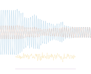
Initially, we wish to comment that the following results only account for multiple-scattering effects present in shallow water and do not account for other non-negligible sources of attenuation such as bed friction and other sources of physical dissipation. We start by illustrating the numerical solution from a single realisation of a random bed. In figure 2 the function  $h(x)/h_0$ is plotted about $-$2 on the vertical scale in the figure which is used to represent the real and imaginary parts of the pseudo-potential. In this simulation the bed is defined by $h_0 = 1$, $\varLambda = 2h_0$, $\sigma ^2 = 0.02$ and $L = 400h_0$. The figure illustrates the randomness of the wave response over the bed and partial reflection and transmission of the incident wave. Note that partial transmission is not necessarily a result of wave attenuation over the random bed and occurs whenever there are changes in propagation characteristics. See, for example, the results of Mei & Black (Reference Mei and Black1969) for wave propagation over a rectangular step.

Figure 2. An example of the pseudo-potential (real and imaginary parts of  $\varOmega (x)$) and an overlay of the random function representing bathymetry $0 < x < L$. Here, $\sigma ^2 = 0.02$, $\varLambda =2h_0$ and $L=400h_0$.
We should also mention that the function describing the random beds are stored numerically at discrete points at a sufficiently high resolution that linear interpolation can be used to accurately represent  $h(x)$ and $h'(x)$ at any intermediate points needed by the numerical integration routine.
In figure 3 we present plots illustrating the typical convergence of the dimensionless attenuation rate,  $h_0 \langle k_i \rangle$, against $N$, the number of simulations. In both plots, the bed is of fixed length of $L = 400h_0$ with vertical variations parametrised by $\sigma ^2 = 0.02$. In one plot we fix frequency at $k_0 \varLambda = 1$ and vary $\varLambda /h_0 = 1,2,4,8$. In the second plot we fix $\varLambda /h_0 = 4$ and vary $k_0 \varLambda = 0.5,1,2,4$. Similar results are found when $\sigma$ is varied with $\varLambda /h_0$ and $k_0 \varLambda$ are held fixed. These and other tests performed suggest $N=500$ simulations is sufficiently large to obtain reasonable convergence to the ensemble average when balanced against computational time. We use $N=500$ by default occasionally increasing $N$ when there is good reason to do so. Generally we find convergence is faster for larger $k_0 \varLambda$ and for larger $\varLambda /h_0$ and smaller values of $\sigma$.

Figure 3. Variation of the dimensionless attenuation constant as  $N$, the number of simulations, increases for random bathymetry with $L=400h_0$ and $\sigma ^2 = 0.02$. In (a) $k_0\varLambda =1$ is fixed and $\varLambda /h_0$ is varied; in (b) ${\varLambda /h_0 = 4}$ is fixed and $k_0 \varLambda$ is varied.
The next issue we address is the effect of bed length on convergence of the attenuation rate computed from the numerical simulation. In figure 4 we have fixed the bed statistics to  $\sigma ^2 = 0.02$, $\varLambda /h_0 = 2$ and plotted the ensemble average of dimensionless attenuation coefficient against $k_0 \varLambda$ for bed lengths increasing from $L = 80h_0$ to $2000h_0$. Overlaid is the theoretical prediction for a semi-infinite bed given by (4.32). Thus, in figure 4, the numerical simulations appear to be converging to the theory as $L \to \infty$.

Figure 4. Non-dimensional ensemble-averaged attenuation coefficient for  $N=500$ simulations for beds of increasing length $L$, compared with theory. Here, $\sigma ^2 = 0.02$ and $\varLambda =2h_0$.
Figure 4 indicates that the section of variable bed needs to be sufficiently long for multiple wave scattering interactions over the variable bed to accurately capture decay due to randomness. Since this is determined by calculating  $\lambda _{\pm } = {\rm e}^{\mp k_i L}$ for each realisation, it is expected that $L$ will be defined by $k_i L = C$ for a constant $C$ sufficiently large that variations due to randomness in eigenvalues $\lambda _{\pm }$ of the transfer matrix ${\mathsf {P}}$ remain on the real line. Extensive numerical experimentation has indicated that the rule $k_i L = 1$, $k_i$ being the theoretically derived attenuation rate, seem to produce ensemble averages which converge across all frequencies although a small proportion of realisations still return eigenvalues from the transfer matrix indicating no attenuation. However, setting $L$ according to the rule $k_i L = 1$ implies increasingly long beds in both the low- and high-frequency limits. Numerical simulations become both computationally expensive and prone to rounding errors. Instead we have produced results with $L = 10 \varLambda /\sigma ^2$ which has the benefit of being independent of frequency so that the same bed realisations can be used across all frequencies. In doing so we are not able guarantee convergence of numerical results for $k_0 \varLambda$ such that $k_0 \varLambda {\rm e}^{-k_0^2 \varLambda ^2/2} \lesssim 0.05 \sqrt {\varLambda /\sigma ^2 h_0}$. For example, with $\sigma ^2 = 0.01$ and $\varLambda /h_0 = 2$ this translates to $k_0 \varLambda \lesssim 0.7$. Discrepancies between the numerical simulations and theory are noticeable at low frequencies especially for $\sigma ^2 = 0.01$ in the plots in figure 5. The issue of $L$ not being sufficiently large for high frequencies does not appear to affect the results so much. Similar general comments apply later to figure 10, although we do note the lack of convergence at high frequencies in the case where $L$ takes its lowest value.

Figure 5. Scaled ensemble-averaged attenuation coefficients for  $N=500$ simulations for beds of length $L = 10\varLambda /\sigma ^2$, compared with theory: (a) $\varLambda /h_0 = 2$; (b) $\varLambda /h_0 = 4$.
In figure 5 we collapse simulated data for different values of  $\sigma ^2 = 0.01,0.02,0.04$ onto the theoretical predictions for the scaled attenuation $\varLambda \langle k_i \rangle /\sigma ^2$ for two values of $\varLambda /h_0 = 2,4$. The only differences in the two theoretical predictions are due to the scaling $C_1^2$ which depends on both $k_0 \varLambda$ and $\varLambda /h_0$. Although there is noise in the data, we have confirmed through extensive runs of the model that the fit between the data and the theory improves as $\sigma ^2$ tends to zero. This is expected since the theoretical attenuation is a leading order result from an asymptotic expansion in $\sigma ^2$. The numerical results in figure 5 appear similar in character to results produced by Bennetts et al. (Reference Bennetts, Peter and Chung2015) in their figure 5 where they highlighted the discrepancy between decay experienced by individual realisations and the decay predicted by their theory. These authors correctly surmise: ‘We deduce that the dominant source of attenuation of the effective wave elevation is wave cancellation (decoherence)’. In our analysis, we identified and removed the terms which give rise to this ‘fictitious decay’.
In figure 6 we show ensemble average of the modulus of the transmission coefficient against frequency for beds with statistics  $\sigma ^2 = 0.02$, $\varLambda /h_0 = 2$ in one plot and $\varLambda /h_0 = 4$ in the second, for different lengths $L/h_0 = 100$, 200 and 400. The limit $L \to \infty$ results in $T_\infty = 0$, so the convergence to this limit with increasing $L$ is slow and the variations with $L$ are significant. Results have been produced by averaging over 20 000 simulations to produce much more accurate averages than in previous results. This is done to give a clear indication of the fit between the numerical results for $\langle |T_L| \rangle$ for beds of finite length $L$ and an approximate fit given by the curve $\langle |T_L| \rangle = {\rm e}^{-k_i L}$ where $k_i$ is the attenuation rate defined by (4.32) for a semi-infinite bed. We offer no formal theoretical basis for this ‘model’ fit, but note it agree with exact results in both limits $L\to 0$ and $L \to \infty$. Heuristically, this fit might be explained by the reflection at the junctions at $x=0$ and $x=L$ between varying and constant depths being weak in comparison to the accumulated attenuation via multiple scattering over the length of random bed.

Figure 6. Variation with frequency of the ensemble average of the modulus of the transmission coefficient for  $N=20\,000$ random bed simulations with statistical properties: (a) $\sigma ^2 = 0.02, \varLambda = 2h_0$; (b) $\sigma ^2 = 0.02, \varLambda = 4h_0$. Model refers to the curve fit $\langle |T_L| \rangle = {\rm e}^{-{k_iL}}$.
Another model fit has been found for the ensemble average of the reflection coefficient for scattering over random beds of finite extent. These results are shown in figure 7 for beds of different lengths with  $N=20\,000$ simulations used for averaging. The model fit $\langle |R_L| \rangle = \sqrt {1 - {\rm e}^{-{\sqrt {2}k_iL}}}$ to these results has no theoretical basis but appears to be remarkably accurate. We felt it useful to present this result in the event that it might have practical use or help develop new theoretical results for scattering over random beds of finite extent.

Figure 7. Ensemble average of the reflection coefficient for  $N=20\,000$ simulations of random beds of varying length with statistics: (a) $\sigma ^2 = 0.02, \varLambda = 2h_0$; (b) $\sigma ^2 = 0.02, \varLambda = 4h_0$. The model fits are curves given by $\langle |R_L| \rangle = \sqrt {1 - {\rm e}^{-{\sqrt {2}k_iL}}}$.
7. Results for randomly varying ice thickness in water of constant depth
Having presented theory and simulations in the case of variable bathymetry with no ice cover, we now consider a similar analysis of results for a fluid of constant depth  $h_0$ covered with floating broken ice submerged to a variable depth $d(x)$, $0 < x < L$, varying randomly about $d_0$, with constant submergence found in $x < 0$ and $x > L$. The only changes from the previous results come from different definitions for $C_1$ and $k_0$. Figure 8 shows the real and imaginary parts of the pseudo-potential for a single random simulation of the ice submergence $d(x)/d_0$ illustrated in the same plot for which $d_0 = 1$ and $h_0=2d_0$ (the vertical range $(-3,-1)$ is used to represent $(-h_0,0)$). Again, we observe the signature of partial transmission and reflection in the elevation and note the random response of the pseudo-potential through the variable broken ice cover.

Figure 8. An example of the pseudo-potential (real and imaginary parts of  $\varOmega (x)$) and an overlay of the random function representing ice submergence across $0 < x < L$. Here, $\sigma ^2 = 0.02$, $\varLambda =2d_0$ and $L=400d_0$ and the fluid depth is $h_0 = 2 d_0$.
Figure 9 illustrates how the ensemble average of the attenuation coefficient converges with  $N$, the number of numerical simulations. Each curve is computed from a single set of realisations for particular parameters, but is typical of results across a range of parameters and convergence is identical in character to results for random bathymetry. The depth of the water in these and later results, chosen as $h_0 = 2d_0$ may seem small for a physical setting. The primary role of the depth is in setting the wavenumber $k_0$ in terms of the frequency, $K$. The choice $h_0 = 2d_0$ allows us to extend the range of values of $K$ over which the results can be presented without violating the assumptions of shallowness.

Figure 9. Variation of the non-dimensional attenuation coefficient with increasing  $N$, the number of simulations in the case of randomly varying ice thickness with $\sigma ^2 = 0.02$, $L=400d_0$ and $h_0 = 2 d_0$. In (a) $k_0\varLambda =1$ is fixed and $\varLambda /h_0$ is varied; in (b) $\varLambda /h_0 = 4$ is fixed and $k_0 \varLambda$ is varied.
Figure 10 shows results which are analogous to those obtained in figure 5, comparing the attenuation coefficient calculated by ensemble-averaging numerically determined decay over 500 realisations of a long finite variable ice cover against theoretical results. The vertical axis is scaled so that results for different values of  $\sigma$ can be collapsed onto a single theoretical curve. The results for random ice cover differ from those for random bathymetry only in the definition of $k_0$ and $C_1$ for ice.

Figure 10. Scaled attenuation coefficient averaged over  $N=500$ simulations of random ice over distance defined by $L = 10 \varLambda /\sigma ^2$ compared with theoretical predictions. Here, $h_0 = 2d_0$, $\sigma$ is varied (see legend) and (a) $\varLambda =2d_0$ and (b) $\varLambda =4d_0$.
7.1. Relationship with other models and field data
The shallow-water setting and the low-frequency homogenisation used to replace floes of small finite width by a continuum implies that it is inappropriate to make direct comparisons with field data and existing theoretical models especially at very low or high frequencies. However, it is useful to comment on the general features exhibited by our model of wave propagation through broken ice.
The average attenuation coefficient (4.32) scales like  $k_0^2$ for $k_0 \varLambda \ll 1$ (i.e. at low frequencies) and since $k_0 \propto \omega$ from (2.2) in the shallow-water setting, the attenuation scales like $\omega ^2$ at low frequencies. The attenuation coefficient peaks at $k_0 \varLambda \approx 1$ and then decays exponentially for $k_0 \varLambda > 1$. One of the requirements of homogenisation is that $d(x)$ varies sufficiently slowly and not significantly faster than the wavelength. This translates into the condition $k_0 \varLambda \not \ll 1$ and so the peak in the attenuation is consistent with the assumptions of the model.
Ongoing work which extends the shallow-water theory presented here to deep water (but retaining a homogenisation of the ice floe cover) results in attenuation which is proportional to  $\omega ^8$ at low frequencies, whilst a peak and a high-frequency exponential tail remains.
There has been longstanding interest (see, for example, Squire et al. Reference Squire, Dugan, Wadhams, Rottier and Liu1995) in developing a plausible model which captures the relationship between wave frequency and attenuation observed in field measurements. Analysis of historical data by Meylan et al. (Reference Meylan, Bennetts, Mosig, Rogers, Doble and Peter2018) suggest attenuation scales like  $\omega ^n$ for $n$ between 2 and 4 with variations away from this at high and low frequencies. A simple power-law relationship across all frequencies and all ice conditions may therefore not be appropriate. Attenuation of wave energy as it propagates over shallow water or through broken ice is contributed to by both multiple-scattering-induced localisation and natural physical dissipation. The primary driver of attenuation in broken ice is unclear (see, e.g. Bennetts & Squire Reference Bennetts and Squire2012; Meylan et al. Reference Meylan, Horvat, Bitz and Bennetts2021) and this paper has only attempted to evaluate multiple-scattering effects. Previous attempts at modelling of attenuation based on multiple scattering through variations in ice thickness (see, e.g. figure 4 of Squire et al. Reference Squire, Vaughan and Bennetts2009; Meylan et al. Reference Meylan, Horvat, Bitz and Bennetts2021) suggest that, at very low frequencies, the attenuation may scale like $\omega ^n$ where $n$ is between 8 and 10. However, neither these studies nor other multiple-scattering models (see the discussion in the introduction) have captured a peak and ‘rollover effect’ in the attenuation at higher frequencies as we have done in our theory. This may be because the onset of rollover occurs at frequencies beyond the limitations of our theory. It may also be due to differences in how the multiple-scattering calculations are made in this work compared with others. Beyond the assumptions of homogenisation we make no other approximation to the scattering process within the ice. In the work of Squire et al. (Reference Squire, Vaughan and Bennetts2009), for example, it is typical that the ice is modelled as a thin elastic plate with no draft and that scattering is calculated using a serial approximation (see Williams Reference Williams2006) which effectively neglects reflections at ice floe interfaces and is based on wide-spacing approximations. In particular, this latter assumption formally requires breaks in the ice to be large compared with the wavelength and is complementary to our assumption.
The rollover effect that appears in our theory of random multiple scattering has been a feature of many sets of field measurements taken in the marginal ice zones. See, for example, Squire et al. (Reference Squire, Dugan, Wadhams, Rottier and Liu1995), who include field measurements of Wadhams et al. (Reference Wadhams, Squire, Goodman, Cowan and Moore1988) and Liu et al. (Reference Liu, Vachon, Peng and Bhogal1992) in which attenuation is observed to peak and start to drop as the frequency increases beyond a critical value. High-frequency rollover effects have since been disputed, most notably in Rogers et al. (Reference Rogers, Thomson, Shen, Doble, Wadhams and Cheng2016) and Thomson et al. (Reference Thomson, Hošeková, Meylan, Kohout and Kumar2021) who attributes rollover to a statistical effect in data analysis. Thus, Thomson et al. (Reference Thomson, Hošeková, Meylan, Kohout and Kumar2021) consider a synthetic (not floating ice) problem in which the attenuation is known and show that measurements fail to replicate the expected high-frequency behaviour and, instead, exhibit a rollover effect.
8. Conclusions
The paper has considered a basic model for the propagation of long waves through water of variable shallow depth with a surface covered by fragmented broken ice. Simple expressions have been derived for the attenuation of waves over randomly varying bathymetry and through ice of randomly varying thickness. In the analytic derivation of the expression for attenuation based on randomness occupying a semi-infinite domain, we have identified and removed terms responsible for incoherent phase cancellations in the ensemble-averaging process which contribute to fictitious decay not experienced by individual realisations of wave propagation through randomness. The theory has been shown to agree with numerical simulations in which averaging was performed over individual wave realisations across randomness of finite extent. In the simulations, for which our shallow-water models require numerical solutions to simple two-dimensional ODEs, attenuation was measured accurately by computing eigenvalues of the resulting transfer matrix. These encode propagation but exclude multiple scattering effects relating to transitions at the ends of the scattering region from variable to constant parameter values.
In addition to resolving the discrepancy between theory and numerical simulations for random bathymetry highlighted by Bennetts et al. (Reference Bennetts, Peter and Chung2015), we have also shown that there is a peak in attenuation which relates closely to a Bragg resonant effect, the significant length scale of the bed being its statistical correlation length. Beyond this peak, attenuation decreases exponentially as a function of the square of the wavenumber. This decay, predicted by the shallow-water model, therefore appears not to be a finite-depth effect as proposed in some previous studies (e.g. Devillard et al. (Reference Devillard, Dunlop and Souillard1988) and Mei et al. (Reference Mei, Stiassnie and Yue2005, § 5)).
The shallow-water formulation has been extended to include the effect of broken ice using the method of Porter (Reference Porter2019). This second-order extension of the classical shallow-water model includes vertical acceleration which is needed for the ice thickness to enter the dynamics. Agreement has been confirmed between theory and numerical simulations.
Whilst our model may not be applicable to field data due to it being highly simplified, it does provide evidence for a key, albeit disputed, feature of the data sets in that of a ‘rollover effect’. This gives us reason to believe that random variations in ice thickness could be a plausible mechanism for the attenuation of waves through broken sea ice; however, as the sea ice is multi-phase and non-continuous and our model is limited to a shallow-water model in a continuum ice cover limit, further work is needed to establish greater certainty. We plan a range of extensions to the current work to include more complex effects which include: (i) finite water depth; (ii) variable ice cover concentration; (iii) discrete ice floe models; (iv) weak nonlinearity; and (v) three-dimensional scattering.
Funding
L.D. is grateful for the support of an EPSRC (UK) studentship.
Declaration of interests
The authors report no conflict of interest.
Data availability statement
The data used to produce the figures in this study are openly available at https://doi.org/10.6084/m9.figshare.23912769.v2
Appendix. Derivation of the long-wave model
The model will be developed in a two-dimensional Cartesian framework  $(x,z)$ with $z$ directed vertically upwards. Fluid of density $\rho$ is bounded below by a rigid bed located at $z=-h(x)$ and above by freely-floating fragmented ice of thickness $d(x) \rho /\rho _i$ where $\rho _i$ is the density of ice. The moving fluid/ice interface is described by $z = -d(x) + \zeta (x,t)$ where $\zeta (x,t)$ represent the wave elevation and $t$ is time. Thus, the rest position of an unloaded fluid surface would be $z=0$.
We assume that the depth is small compared with the wavelength and that gradients of  $h(x)$ and $d(x)$ are equally small. The ice is assumed broken into individual floes whose horizontal extent is small compared with the wavelength. The floes are constrained to move vertically. The length of individual floes does not enter our model since we assume a continuum model from the outset (the description of the ice submergence as $d(x)$ already indicates this) which avoids engaging in a formal derivation based on multiple horizontal scales.
The fluid is assumed to be both inviscid and incompressible and its motion is represented by the velocity field  $(u(x,z,t),w(x,z,t))$, $u$ and $w$ being the horizontal and vertical components of the flow, respectively.
Within the fluid, conservation of mass requires
 \begin{equation} u_x + w_z = 0 \end{equation}
is satisfied. Conservation of momentum gives
 \begin{equation} \rho u_t + \rho (u u_x + w u_z) ={-}p_x,\quad \mbox{and}\quad \rho w_t + \rho (u w_x + w w_z) ={-}p_z, \end{equation}
where  $p(x,z,t)$ is the dynamic pressure in the fluid in excess of background hydrostatic pressure $-\rho g z$, where $g$ is acceleration due to gravity and the background atmospheric pressure above the ice is assumed without loss of generality to be zero. On the rigid bed, the no-flow condition is represented by
 \begin{equation} w + h'(x) u = 0,\quad \mbox{on } z ={-}h(x), \end{equation}
and on the moving fluid/ice interface we have the kinematic and dynamic conditions
 \begin{equation} \zeta_t = w + (d'(x)-\zeta_x(x,t)) u,\quad \mbox{on } z ={-}d(x) + \zeta(x,t), \end{equation}
and
 \begin{equation} \rho d(x) \zeta_{tt} = p(x,-d(x)+\zeta(x,t),t) - \rho g \zeta(x,t). \end{equation}
We rescale physical variables using
 \begin{equation} x = Lx^*,\quad z = Hz^*,\quad h=Hh^*,\quad d=Hd^*\quad \mbox{and}\quad \zeta = A\zeta^*, \end{equation}
where  $L$ represents a characteristic horizontal length scale (a different definition from that used in the main text for the length of the bed) associated with the wavelength and/or the variable bed/ice cover, $H$ is a characteristic fluid depth and $A$ a characteristic wave elevation. We also define
 \begin{equation} \epsilon = \frac{H}{L},\qquad \delta=\frac{A}{H}, \end{equation}
which represents shallowness and linearisation parameters, respectively. We suppose that both  $\epsilon$ and $\delta$ are small and assume that $\delta =o(\epsilon ^2)$ to ensure we operate within a linearised setting.
Based on the shallow-water dispersion relation, we select a time scale  $T=L/\sqrt {gH}$ so that $t= Lt^*/\sqrt {gH}$ and set
 \begin{equation} u = \frac{A}{H}\sqrt{gH}u^* \quad \mbox{and} \quad w = \frac{A}{L}\sqrt{gH}w^* \end{equation}
whilst  $p = \rho g A p^*$. Under this change of variables the governing equations become (after dropping asterisks)
 \begin{equation} u_{x} + w_{z} = 0 \end{equation}
with
 \begin{equation} u_{t} + \delta (u u_{x}+w u_{z}) ={-}p_{x} \end{equation}
and
 \begin{equation} \epsilon^2 w_{t} + \delta \epsilon^2 (u w_{x}+w w_{z}) ={-}p_{z}. \end{equation}
Our boundary condition at the fluid bed reads
 \begin{equation} w + h'(x) u = 0 \quad \mbox{on } z={-}h(x), \end{equation}
with our boundary conditions on the ice becoming
 \begin{equation} \zeta_{t} = w + (d'(x) - \delta\zeta_x(x,t)) u,\quad \mbox{on } z ={-}d(x) + \delta \zeta(x,t) \end{equation}
and
 \begin{equation} \epsilon^2 d(x) \zeta_{tt} = p(x,-d(x) + \delta\zeta(x,t),t)- \zeta. \end{equation}
Noting that  $\delta = o(\epsilon ^2)$ has been assumed we expand variables up to $O(\epsilon ^2)$, so that
 \begin{equation} \zeta(x,t) = \zeta^{(0)}(x,t) +\epsilon^2\zeta^{(1)}(x,t) +\cdots \end{equation}
and
 \begin{equation} \{\, p,u,w\}(x,z,t) =
\{\,p^{(0)}, u^{(0)}, w^{(0)} \}(x,z,t) +\epsilon^2 \{\, p^{(1)}, u^{(1)}, w^{(1)} \}(x,z,t) +
\cdots.\end{equation}
\begin{equation} \{\, p,u,w\}(x,z,t) =
\{\,p^{(0)}, u^{(0)}, w^{(0)} \}(x,z,t) +\epsilon^2 \{\, p^{(1)}, u^{(1)}, w^{(1)} \}(x,z,t) +
\cdots.\end{equation}
Only in the case that  $h(x)$ and/or $d(x)$ contain discontinuities would we need to include terms of $O(\epsilon )$ (see Mei et al. (Reference Mei, Stiassnie and Yue2005, § 5)) since these would arise from an asymptotic matching process across the discontinuity. It is consistent with this expansion that we neglect contributions from terms multiplying $\delta$ in (A9)–(A14). We continue by solving for the leading-order variables. From (A11), $p^{(0)}_z = 0$ and from (A14), $p^{(0)}(x,-d(x),t) = \zeta ^{(0)}(x,t)$ implies
 \begin{equation} p^{(0)}(x,z,t) = \zeta^{(0)}(x,t) \end{equation}
and then from (A10) we have
 \begin{equation} u_t^{(0)}(x,z,t) ={-}\zeta^{(0)}_x(x,t) \end{equation}
and so  $u^{(0)}$ is a function of $x$ and $t$ only. Integrating (A9) at leading order from $z=-h(x)$ to $z=-d(x)$ and using (A12) and (A13) gives
 \begin{equation} q^{(0)}_x(x,t) = ((h(x)-d(x))u^{(0)}(x,t))_x ={-}\zeta_t^{(0)}(x,t) ,\end{equation}
where we have defined the depth-integrated horizontal fluid flux  $q(x,t) = q^{(0)}(x,t) + \epsilon ^2 q^{(1)}(x,t) + \cdots$ with
 \begin{equation} q^{(0,1)}(x,t) = \int_{{-}h(x)}^{{-}d(x)} u^{(0,1)} (x,z,t) \,{\rm d} z. \end{equation}
Eliminating between (A18) and (A19) gives either
 \begin{equation} \zeta_{tt}^{(0)} = ((h(x)-d(x)) \zeta^{(0)}_x)_x, \quad \mbox{or}\quad q_{tt}^{(0)} = (h(x)-d(x)) q_{xx}^{(0)} \end{equation}
as the leading-order governing equation, expressed in dimensionless variables. That is, the effect of fragmented ice cover at leading order is equivalent to an uncovered fluid having a reduced depth,  $h(x)-d(x)$.
Now we work at the next order,  $O(\epsilon ^2)$. Integrating (A9) at order $O(\epsilon ^2)$ from $z=-h(x)$ to $z=-d(x)$ and using (A12) and (A13) at $O(\epsilon ^2)$ gives
 \begin{equation} q^{(1)}_x(x,t) = \frac{\partial}{\partial x} \int_{{-}h(x)}^{{-}d(x)} u^{(1)}(x,z,t) \,{{\rm d}\kern0.7pt x} ={-} \zeta_t^{(1)}(x,t). \end{equation}
The next step is to determine the leading-order vertical velocity integrating (A9) again, but now from  $z$ to $-d(x)$, to give
 \begin{equation} w^{(0)}(x,z,t) = \zeta^{(0)}_t(x,t) - ((z+d(x)) u^{(0)}(x,t))_x ,\end{equation}
which is linear in  $z$. From (A11) at $O(\epsilon ^2)$ we infer that
 \begin{equation} p^{(1)}_z(x,z,t) ={-}\zeta_{tt}^{(0)} + ((z+d(x)) u_t^{(0)})_x ,\end{equation}
which can be integrated using the condition (A14) at  $O(\epsilon ^2)$ to give
 \begin{equation} p^{(1)}(x,z,t) = \zeta^{(1)} - z \zeta_{tt}^{(0)} + \tfrac12 ((z+d(x))^2 u_t^{(0)})_x. \end{equation}
Using this in (A10) at  $O(\epsilon ^2)$ gives
 \begin{equation} u_t^{(1)}(x,z,t) ={-}p_x^{(1)} = z \zeta_{ttx}^{(0)} -\zeta^{(1)}_x - \tfrac12 ((z+d(x))^2 u_t^{(0)})_{xx}. \end{equation}
We find, after extensive algebra, which makes repeated use of the relation  $q^{(0)}_t = (h-d) u^{(0)}_t$, that
 \begin{align} q_t^{(1)}(x,t) &= \int_{{-}h(x)}^{{-}d(x)} u^{(1)}_t \,{\rm d} z = \frac12 (d^2-h^2) \zeta_{ttx}^{(0)} - (h-d) \zeta_x^{(1)} + \frac12 (h-d) d'' q_t^{(0)} \nonumber\\ &\quad -\frac16 \{(h-d)' q_{xxt}^{(0)} -2 (h-d)(h'-d') q_{xt}^{(0)} \nonumber\\ &\quad -(h''-d'') (h-d) q_t^{(0)} +2 (h'-d')^2 q_t^{(0)}\} \nonumber\\ &\quad - {d'}^2 q_t^{(0)} + d' \{ (h-d)q_{xt}^{(0)} - (h' - d') q_t^{(0)}\}. \end{align}
Further simplification and use of the relation  $q_x^{(0)} = -\zeta _t^{(0)}$ results in
 \begin{align} q_t^{(1)} &={-} (h-d) \left(\zeta^{(1)}_x + \tfrac13 \left( (h + 2d) \zeta_{tt}^{(0)} \right)_x\right) \nonumber\\ &\quad + q_t^{(0)} \left(\tfrac16 (h-d) (h + 2 d)'' - \tfrac13 (h-d)'(h+2d)' -d'^2\right). \end{align}
We can now recombine leading order and  $O(\epsilon ^2)$ terms as we redimensionalise variables, a process which leads to the coupled equations
 \begin{equation} \zeta_t ={-} q_x \end{equation}
and
 \begin{align} & \left(1 +d'^2 + \frac13 (h-d)'(h+2d)' - \frac16 (h-d) (h + 2 d)'' \right) q_t \nonumber\\ &\quad ={-}(h-d) \left( g \zeta + \frac{(h+2d)}{3} \zeta_{tt} \right)_x \end{align}
expressed in terms of the original physical variables  $q$ and $\zeta$ and which are accurate to $O(\epsilon ^2)$. Eliminating $q$ in favour of $\zeta$ gives us the governing equation
 \begin{equation} \zeta_{tt} = \frac{\partial}{\partial x} \left( \hat{d}(x) \frac{\partial}{\partial x} \left( g \zeta + \frac{(h+2d)}{3} \zeta_{tt} \right) \right) ,\end{equation}
where
 \begin{equation} \hat{d}(x) = \frac{(h-d)}{1 +d'^2 - \dfrac16 (h-d)(h+2d)'' + \dfrac13 (h-d)'(h+2d)'}. \end{equation}
Note that when  $d(x) \equiv 0$ we recover (2.13) from Porter (Reference Porter2019). We see that the expansion to $O(\epsilon ^2)$ in the small parameter $\epsilon = H/L$ has captured the contribution from the inertia of the ice in (A31) whilst there are non-trivial modifications to the wave speed through the geometrical factors associated with varying $d(x)$ and $h(x)$ in (A32). Specifically, it is worth noting that $(h+2d)/3 = (h-d)/3 + d$ and $h-d$ is the vertical extent of the fluid. Thus, the isolated contribution $d \zeta _{tt}$ is associated with ice inertia and the remaining $\frac 13 (h-d) \zeta _{tt}$ is a contribution from vertical acceleration of the fluid through depth-averaging, in common with Porter (Reference Porter2019).
Eliminating  $\zeta$ in favour of $q$ between (A29) and (A30) gives
 \begin{equation} q_{tt} = \hat{d}(x) \left( g q_x + \frac{(h+2d)}{3} q_{ttx} \right)_x \end{equation}
and this provides the starting point for a series of transformations of the dependent variable which follow Porter (Reference Porter2019). We factorise a time-harmonic variation with
 \begin{equation} q(x,t) = {\rm Re} \left\{ \frac{\varphi(x)}{\sqrt{1- \dfrac13 K (h + 2d)}}{\rm e}^{-\mathrm{i} \omega t}\right\} \end{equation}
and the square-root factor in the denominator simultaneously transforms the resulting ODE into canonical form. Thus, after some algebra we find
 \begin{equation} \varphi''(x)+\left(\frac{\hat{K}}{h-d}\left(1+\frac13 v_1(h,d) h'(x)^2 + \frac13 v_2(h,d) (d'(x)^2 + h'(x)d'(x))\right)\right)\varphi(x) = 0 ,\end{equation}
where
 \begin{gather} \hat{K} = \frac{K}{1 - \dfrac13 K (h + 2d)}, \end{gather}
 \begin{gather}v_1(h,d) = 1 + \frac{1}{12}\hat{K}(h(x)-d(x)) \quad \mbox{and}\quad v_2(h,d) = 1 + \frac{1}{3}\hat{K}(h(x)-d(x)). \end{gather}
 A final change of variables is made, by letting  $\varOmega (x)=\varphi '(x)$ and it follows that (A35) is transformed into
 \begin{equation} ({\hat {\hat d}}(x) \varOmega')' + K \varOmega = 0, \end{equation}
where
 \begin{equation} {\hat {\hat d}}(x) = \frac{(h-d)\left(1-\dfrac{1}{3}K(h+2d)\right)}{1+\dfrac13 v_1(h,d) h'(x)^2 + \dfrac13 v_2(h,d) (d'(x)^2 + h'(x)d'(x))}. \end{equation}
This final series of transformations have brought about two useful features. The first is that (A38) is expressed in a form aligned with the familiar linearised first-order shallow-water equation. The second is that the function  $\varOmega (x)$ and its derivative $\varOmega '(x)$ are continuous even if $h'(x)$ and/or $d'(x)$ are discontinuous. The loaded surface can be reconstructed from $\varOmega (x)$ by following the effect of each transformation and turns out to be represented by
 \begin{align} \eta &= \frac{(-{\rm i}/\omega)}{\sqrt{1-\dfrac{1}{3}K(h+2d)}} \nonumber\\ &\quad \times\left(\varOmega(x)-\frac{\dfrac{1}{6}(h-d)(h+2d)'}{1+\dfrac13 v_1(h,d) h'(x)^2 + \dfrac13 v_2(h,d) (d'(x)^2 + h'(x)d'(x))}\varOmega'(x)\right) , \end{align}
where  $\zeta (x,t) = \textrm {Re} \{ \eta (x) {\rm e}^{-\mathrm {i} \omega t}\}$.
Since we anticipate  $K h \ll 1$, we can make approximations $v_1(h,d) \approx 1$ and $v_2(h,d) \approx 1$, noting $0< h-d\leq h$ and so
 \begin{align} \tfrac13 v_1(h,d) h'(x)^2 + \tfrac13 v_2(h,d) (d'(x)^2 + h'(x)d'(x))\approx \tfrac13 (h'(x)^2+h'(x)d'(x) + d'(x)^2). \end{align}
We note that if we let  $d(x)=0$ in (A39), (A40) and (A41), we recover expressions derived in Porter (Reference Porter2019).


 Open access