


Nomenclature
- $\textbf{H}(\textbf{q})$
-
positive definite symmetric inertia matrix
-
$\textbf{C}(\textbf{q},\dot{\textbf{q}})$
-
coriolis and centrifugal matrix
-
$\textbf{q},\dot{\textbf{q}},\ddot{\textbf{q}}$
-
generalized position, velocity and acceleration vector
-
$\textbf{u}$
-
the input control torque
-
$\textbf{u}_c$
-
the desired torque command
-
$\textbf{d}$
-
represent the bounded disturbaces
-
$\textbf{e}_1$
-
trajectory tracking error
-
$\textbf{e}_2$
-
velocity tracking error
-
$\textbf{s}$
-
sliding surface
-
$\textbf{f}_{\textrm{dis}}$
-
unknown lumped uncertain term
-
$\textbf{q}_d$
-
the desired motion trajectory
-
$\dot{\textbf{q}}_d$
-
the desired motion velocity trajectory
-
$b_c, b_n, b_m, a_n, b_1, b_2, b_3, b_4$
-
positive constants
-
$c_1, c_2, c_3$
-
unknown constants
-
$m_1, n_1$
-
positive constants
-
$p,q$
-
positive odd integers
-
$\rho$
-
a positive continuous function
-
$\textbf{K}_1, \textbf{K}_2, \boldsymbol{\eta}, \boldsymbol\zeta$
-
positive definite matrices
-
$\varepsilon_N$
-
arbitrary small positive constant
-
$\boldsymbol\Omega$
-
auxiliary variable


1.0 Introduction
With the increasing number of orbital debris and failed satellites, space manipulator technologies aimed at active debris removal and on-orbit maintenance have received widespread attention [Reference Flores Abad, Ma, Pham and Ulrich1, Reference Rybus2]. To conserve fuel consumption, the space manipulator applied to on-orbit missions normally has a free-floating spacecraft base. As the spacecraft’s thrusters are turned off, there is a strong coupling between the manipulator and the spacecraft’s base. That is, any movement of the manipulator interferes unfavourably with the translation and rotation of the spacecraft base. Such a characteristic makes the tracking control of the space manipulator more challenging than that of the terrestrial manipulator. Besides, the space manipulator is inevitably subject to parametric uncertainties and environmental perturbations, degrading system control performance and even destabilising the whole system. To address these issues, many control methodologies have been introduced into the trajectory tracking of space manipulators, for instance, adaptive control [Reference Wang and Xie3, Reference Nekoo4], robust control [Reference Jia and Misra5, Reference Seddaoui and Saaj6], sliding mode control(SMC) [Reference Xie, Sun, Kwan and Wu7, Reference Jia, Yuan, Chen and Fu8] and neural network control [Reference Kumar, Panwar and Borm9, Reference Yao10].
The majority of the aforementioned approaches, however, only guarantee the asymptotic stability of tracking errors with infinite convergence time. In pursuit of faster response and higher tracking precision, finite-time control (FTC) schemes have been frequently implemented in the trajectory tracking of manipulators. A terminal sliding mode control (TSMC) was presented for a space rigid manipulator sensitive to external disturbance to accomplish the finite-time state convergence [Reference Guo and Li11]. Feng et al. [Reference Feng, Yu and Man12] constructed a global non-singular terminal sliding mode control (NTSMC) to overcome the singularity problem existing in the traditional TSMCs. Based on adaptive NTSMC, a finite-time trajectory controller was also investigated for a space manipulator considering actuator saturation simultaneously [Reference Jia and Shan13]. In Ref. [Reference Yang and Yang14], a continuous singularity-free fast terminal sliding mode control (FTSMC) was put forward to speed up the convergence rate, especially when the state was far from the equilibrium point. Shao et al. [Reference Shao, Sun, Xue and Li15] proposed NTSMC for the finite-time trajectory tracking of free-floating space manipulator with unknown disturbances, which enhanced the transient performance of the system and reduced the perturbations to the spacecraft base. A continuous non-singular integral sliding mode control (NISMC) was also presented for the finite-time fault-tolerant control of space manipulators to deal with different undesirable actuator faults [Reference Jia and Shan16]. Nevertheless, the settling time required in these FTC schemes is sensitive to the system’s initial conditions, which makes it difficult to obtain a prior accurate estimation of the convergence time. Considering this fact, the concept of fixed-time stabilisation was firstly proposed by Polyakov [Reference Polyakov17]. The significant property of this method is that the upper bound of the settling time is only determined by predefined control parameters regardless of initial states. Due to such an excellent feature, fixed-time control strategies have received a lot of popularity in the field of nonlinear system control [Reference Zuo18–Reference Chen, Wang and Liu21]. In particular, an observer-based fixed-time control scheme was developed for the task-space trajectory tracking of a space manipulator with external disturbances [Reference Jin, Rocco and Geng22]. In Ref. [Reference Su, Zheng and Mercorelli23], a non-singular TSMC was proposed to guarantee the fixed-time tracking stabilisation of a robot manipulator system despite parameter uncertainties and external disturbances. By combining an adaptive mechanism, a non-singular fixed-time SMC scheme was then developed for trajectory tracking of an uncertain manipulator under actuator saturation [Reference Sai, Xu, He, Zhang and Zhu24].
Whilst the transient performance, which is crucial to executing the task of trajectory tracking, has been overlooked in the aforementioned efforts. Due to the absence of prior information about the distant environment or objects, the system states should be restricted to specific predefined ranges to avoid accidental collisions between the space manipulator and objects. Therefore, it is necessary to take the impact of output state constraints on system performance into consideration. An adaptive fuzzy neural network (NN) control was derived for a constrained robot [Reference He and Dong25], where a barrier Lyapunov function was employed for performance improvement. The barrier Lyapunov function technique solely focuses on the qualitative treatment of boundary constraints rather than the quantitative evaluation of dynamic performance constraints. As is well known, the PPC [Reference Bechlioulis and Rovithakis26] is an appropriate choice for quantitatively characterising dynamic and steady-state performances in advance. The tracking error is confined in this approach inside the envelope described by the specified performance function, so as to achieve the desired transient and steady-state performances. Its primary idea is the use of error transformation to transform the original constrained dynamics into an equivalent unconstrained one. Thereby, the performance metrics, such as convergence time, steady-state error and overshoot, are assured to satisfy the predefined requirements on the premise of preserving the unconstrained system’s stability. The concept of prescribed performance was first applied in the funnel control (FC) proposed in Ref. [Reference Ilchmann, Ryan and Townsend27]. Compared with PPC, FC is usually limited to nonlinear systems with a relatively low-degree. Therefore, in recent years, PPC has been widely utilised in the control of robotic systems [Reference Kostarigka, Doulgeri and Rovithakis28, Reference Psomopoulou, Theodorakopoulos, Doulgeri and Rovithakis29], space vehicle systems [Reference Bu, Xiao and Lei30, Reference Bu, Wu, Huang and Wei31] and multi-agent systems [Reference Bechlioulis and Rovithakis32], for the sake of ensuring the system’s desired transient performance. And a new finite-time PPC (FPPC) is exploited in Ref. [Reference Bu, Qi and Jiang33], which enables given-time convergence of tracking errors with small overshoot. Moreover, several studies have been conducted on the issue of tracking control for space manipulators considering prescribed performance constraints [Reference Zhou, Zhang and Zhou34–Reference Lu and Jia36]. Although there are promising advances in the tracking control of space manipulators with specified performance, the existing methods have the following shortcomings:
-
(1) There is a sluggish transient response, and large convergence time is necessary when system state is far from the equilibrium point.
-
(2) The structure of PPC-based constraint controllers [Reference Ma, Zhou, Li and Lu37–Reference An, Chen, Wang and Wu39] is usually extremely sophisticated due to the full use of transformed error.
-
(3) When considering input saturation, they have difficulty guaranteeing performance constraints and fixed-time tracking convergence.
Inspired by the above observations, a novel adaptive fixed-time control scheme with prescribed performance constraints is developed for trajectory tracking of the free-floating space manipulator subject to input saturation. Parameter uncertainties and unknown disturbances are also considered. More specifically, the main contributions of this paper are concisely summarised as follows:
-
(1) A non-singular fast fixed-time terminal sliding surface is constructed to obtain a faster convergence rate than the existing fixed-time terminal sliding surfaces in Refs [Reference Huang and Jia40, Reference Ni, Liu, Liu, Hu and Li41].
-
(2) To avoid the complexities associated with stabilising transformed error in conventional PPCs, a unique tan-type PPC technique is directly introduced in the control design. The structural simplicity of the designed controller allows for greater flexibility in practical applications.
-
(3) The effect of actuator saturation is mitigated by an input saturation compensator. The resulting controller ensures that the fixed-time prescribed performance of the space manipulator is fulfilled, considering parameter uncertainties, unknown disturbances, and input saturation simultaneously.
The rest of this work is organised as follows. Section 2 represents the problem description and some required definitions. In Section 3, the processes of control design and stability analysis are given in detail. Section 4 discusses the simulation results, and draws conclusions in Section 5.
2.0 Problem description and preliminaries
2.1 Notations and lemmas
For an n-dimensional vector $ x=[{x}_{1},{x}_{2}, \ldots ,{x}_{n}{]}^{\textrm{T}}$
with the
$ x=[{x}_{1},{x}_{2}, \ldots ,{x}_{n}{]}^{\textrm{T}}$
with the $ i$
th element
$ i$
th element $ {x}_{i}$ $ (i=\textrm{1,2}, \ldots ,n)$
. The symbols
$ (i=\textrm{1,2}, \ldots ,n)$
. The symbols $ \parallel \cdot \parallel $
and
$ \parallel \cdot \parallel $
and $ \parallel \cdot {\parallel }_{1}$
represent the Euclidean norm and 1-norm, respectively. For a constant
$ \parallel \cdot {\parallel }_{1}$
represent the Euclidean norm and 1-norm, respectively. For a constant $ \gamma \gt 0$
, define
$ \gamma \gt 0$
, define $ \textrm{s}\textrm{i}{\textrm{g}}^{\gamma }\left(x\right)={\left[|{x}_{1}{|}^{\gamma }\textrm{s}\textrm{i}\textrm{g}\textrm{n}\left({x}_{1}\right),|{x}_{2}{|}^{\gamma }\textrm{s}\textrm{i}\textrm{g}\textrm{n}\left({x}_{2}\right),\dots ,|{x}_{n}{|}^{\gamma }\textrm{s}\textrm{i}\textrm{g}\textrm{n}\left({x}_{n}\right)\right]}^{\textrm{T}}$
and the vector
$ \textrm{s}\textrm{i}{\textrm{g}}^{\gamma }\left(x\right)={\left[|{x}_{1}{|}^{\gamma }\textrm{s}\textrm{i}\textrm{g}\textrm{n}\left({x}_{1}\right),|{x}_{2}{|}^{\gamma }\textrm{s}\textrm{i}\textrm{g}\textrm{n}\left({x}_{2}\right),\dots ,|{x}_{n}{|}^{\gamma }\textrm{s}\textrm{i}\textrm{g}\textrm{n}\left({x}_{n}\right)\right]}^{\textrm{T}}$
and the vector $ \textrm{s}\textrm{g}\textrm{n}\left(x\right)=\left[\textrm{s}\textrm{i}\textrm{g}\textrm{n}\right({x}_{1}),\textrm{s}\textrm{i}\textrm{g}\textrm{n}({x}_{2}), \ldots ,\textrm{s}\textrm{i}\textrm{g}\textrm{n}({x}_{n}){]}^{\textrm{T}}$
, where
$ \textrm{s}\textrm{g}\textrm{n}\left(x\right)=\left[\textrm{s}\textrm{i}\textrm{g}\textrm{n}\right({x}_{1}),\textrm{s}\textrm{i}\textrm{g}\textrm{n}({x}_{2}), \ldots ,\textrm{s}\textrm{i}\textrm{g}\textrm{n}({x}_{n}){]}^{\textrm{T}}$
, where $ \textrm{s}\textrm{i}\textrm{g}\textrm{n}(\cdot )$
denotes the sign function.
$ \textrm{s}\textrm{i}\textrm{g}\textrm{n}(\cdot )$
denotes the sign function. $ {I}_{n}\in {\mathbb{R}}^{n\times n}$
is n-dimensional identity matrix.
$ {I}_{n}\in {\mathbb{R}}^{n\times n}$
is n-dimensional identity matrix.
Lemma 1. [Reference Zuo and Tie42] Let $ {A}_{i}\ge 0(i=\textrm{1,2}, \ldots ,n)$
, for
$ {A}_{i}\ge 0(i=\textrm{1,2}, \ldots ,n)$
, for $ 0 \lt {p}_{1}\le 1$
and
$ 0 \lt {p}_{1}\le 1$
and $ {p}_{2}\gt 1$
, the following inequalities hold
$ {p}_{2}\gt 1$
, the following inequalities hold
 \begin{align}\mathop \sum \limits_{i = 1}^n A_i^{{p_1}} \ge {\left( {\mathop \sum \limits_{i = 1}^n {A_i}} \right)^{{p_1}}},\mathop \sum \limits_{i = 1}^n A_i^{{p_2}} \ge {n^{1 - {p_2}}}{\left( {\mathop \sum \limits_{i = 1}^n {A_i}} \right)^{{p_2}}}\end{align}
Definition 1 (Fixed-time stable). [Reference Polyakov17] Consider the nonlinear system
 \begin{align} \dot{\textbf{z}}(t)=g(\textbf{z}(t)),\textbf{z}(\boldsymbol{0})={\textbf{z}}_{0},g(\boldsymbol{0})=\boldsymbol{0},\textbf{z}\in {\mathbb{R}}^{n}\end{align}
The origin of the system (2) is said to be fixed-time stable if it is finite-time stable and the convergence time $ T\left({\textbf{z}}_{0}\right)$
is bounded for any initial states, that is,
$ T\left({\textbf{z}}_{0}\right)$
is bounded for any initial states, that is, $ \exists {T}_{max}\gt 0$
such that
$ \exists {T}_{max}\gt 0$
such that $ T\left({\textbf{z}}_{0}\right)\le {T}_{max},\forall {\textbf{z}}_{0}\in {\mathbb{R}}^{n}$
.
$ T\left({\textbf{z}}_{0}\right)\le {T}_{max},\forall {\textbf{z}}_{0}\in {\mathbb{R}}^{n}$
.
Lemma 2 (Globally fixed-time stabilisation). [Reference Zuo18] Suppose there exist one Lyapunov function $ V\left(z\right)$
, such that
$ V\left(z\right)$
, such that $ \dot{V}\left(z\right)\le -{\alpha }_{0}{V}^{{\eta }_{0}}\left(z\right)-{\beta }_{0}{V}^{{\Gamma }_{0}}\left(z\right)$
holds with
$ \dot{V}\left(z\right)\le -{\alpha }_{0}{V}^{{\eta }_{0}}\left(z\right)-{\beta }_{0}{V}^{{\Gamma }_{0}}\left(z\right)$
holds with $ {\alpha }_{0},{\beta }_{0}\gt 0$
,
$ {\alpha }_{0},{\beta }_{0}\gt 0$
, $ {\eta }_{0}\gt 1$
, and
$ {\eta }_{0}\gt 1$
, and $ {\Gamma }_{0}\in \left(\textrm{0,1}\right)$
. Then, the equilibrium of system (2) is globally fixed-time stable, and the settling time
$ {\Gamma }_{0}\in \left(\textrm{0,1}\right)$
. Then, the equilibrium of system (2) is globally fixed-time stable, and the settling time $ T\left({z}_{0}\right)$
is bounded by
$ T\left({z}_{0}\right)$
is bounded by $ T\left({z}_{0}\right)\le \frac{1}{{\alpha }_{0}({\eta }_{0}-1)}+\frac{1}{{\beta }_{0}(1-{{\Gamma }}_{0})},\forall {z}_{0}\in {\mathbb{R}}^{n}$
.
$ T\left({z}_{0}\right)\le \frac{1}{{\alpha }_{0}({\eta }_{0}-1)}+\frac{1}{{\beta }_{0}(1-{{\Gamma }}_{0})},\forall {z}_{0}\in {\mathbb{R}}^{n}$
.
Lemma 3 (Practical fixed-time stabilisation). [Reference Wang, Sun and Liang43] Suppose there is a Lyapunov function $ V\left(z\right)$
, and real number
$ V\left(z\right)$
, and real number $ 0 \lt {\vartheta }_{0} \lt \infty $
,
$ 0 \lt {\vartheta }_{0} \lt \infty $
, $ {\alpha }_{0},{\beta }_{0}\gt 0$
,
$ {\alpha }_{0},{\beta }_{0}\gt 0$
, $ {\eta }_{0}\gt 1$
, and
$ {\eta }_{0}\gt 1$
, and $ {\Gamma }_{0}\in \left(\textrm{0,1}\right)$
, such that
$ {\Gamma }_{0}\in \left(\textrm{0,1}\right)$
, such that $ \dot{V}\left(z\right)\le -{\alpha }_{0}{V}^{{\eta }_{0}}\left(z\right)-{\beta }_{0}{V}^{{\Gamma }_{0}}\left(z\right)+{\vartheta }_{0}$
holds. Then, the system (2) is practical fixed-time stable and the system can be stabilised within the residual set containing the equilibrium point in a fixed time. For
$ \dot{V}\left(z\right)\le -{\alpha }_{0}{V}^{{\eta }_{0}}\left(z\right)-{\beta }_{0}{V}^{{\Gamma }_{0}}\left(z\right)+{\vartheta }_{0}$
holds. Then, the system (2) is practical fixed-time stable and the system can be stabilised within the residual set containing the equilibrium point in a fixed time. For $ {\theta }_{1}$
,
$ {\theta }_{1}$
, $ {\theta }_{2}\in \left(\textrm{0,1}\right]$
, the residual set is presented as
$ {\theta }_{2}\in \left(\textrm{0,1}\right]$
, the residual set is presented as $ {D}_{s}=\left\{{lim}_{t\to T}z\left|V\right(z)\le min\left\{{\alpha }_{0}^{-1/{\eta }_{0}}{\left(\frac{{\vartheta }_{0}}{1-{\theta }_{1}}\right)}^{\frac{1}{{\eta }_{0}}},{\beta }_{0}^{-1/{\Gamma }_{0}}{\left(\frac{{\vartheta }_{0}}{1-{\theta }_{2}}\right)}^{\frac{1}{{\Gamma }_{0}}}\right\}\right\}$
and the upper bound of convergence time is given by
$ {D}_{s}=\left\{{lim}_{t\to T}z\left|V\right(z)\le min\left\{{\alpha }_{0}^{-1/{\eta }_{0}}{\left(\frac{{\vartheta }_{0}}{1-{\theta }_{1}}\right)}^{\frac{1}{{\eta }_{0}}},{\beta }_{0}^{-1/{\Gamma }_{0}}{\left(\frac{{\vartheta }_{0}}{1-{\theta }_{2}}\right)}^{\frac{1}{{\Gamma }_{0}}}\right\}\right\}$
and the upper bound of convergence time is given by $ T\left({z}_{0}\right)\le \frac{1}{{\alpha }_{0}({\eta }_{0}-1)}+\frac{1}{{\beta }_{0}(1-{\Gamma }_{0})},\forall {z}_{0}\in {\mathbb{R}}^{n}$
.
$ T\left({z}_{0}\right)\le \frac{1}{{\alpha }_{0}({\eta }_{0}-1)}+\frac{1}{{\beta }_{0}(1-{\Gamma }_{0})},\forall {z}_{0}\in {\mathbb{R}}^{n}$
.
2.2 Space manipulator model
In the presence of disturbances, the dynamic equation of the free-floating space manipulator shown in Fig. 1 can be expressed as [Reference Shao, Sun, Xue and Li15]:
 \begin{align} \textbf{H}\left(\textbf{q}\right)\ddot{\textbf{q}}+\textbf{C}\left(\textbf{q},\dot{\textbf{q}}\right)\dot{\textbf{q}}=\textbf{u}+\textbf{d}(t)\end{align}
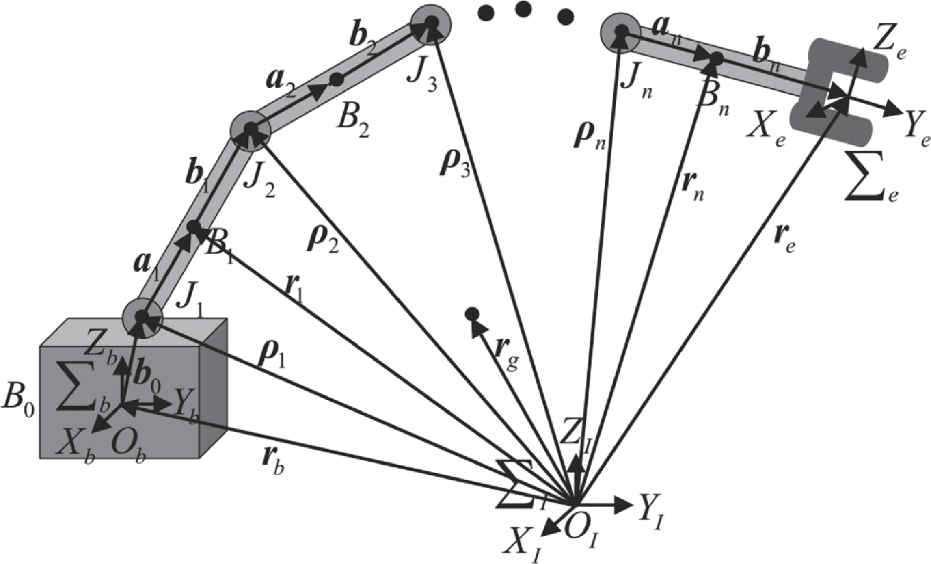
Figure 1. Space manipulator system model.
where, $ \textbf{H}\left(\textbf{q}\right)\in {\mathbb{R}}^{n\times n}$
is the positive definite symmetric inertia matrix.
$ \textbf{H}\left(\textbf{q}\right)\in {\mathbb{R}}^{n\times n}$
is the positive definite symmetric inertia matrix. $ \textbf{C}(\textbf{q},\dot{\textbf{q}})\in {\mathbb{R}}^{n\times n}$
denotes the Coriolis and centrifugal matrix.
$ \textbf{C}(\textbf{q},\dot{\textbf{q}})\in {\mathbb{R}}^{n\times n}$
denotes the Coriolis and centrifugal matrix. $ \textbf{q}$
,
$ \textbf{q}$
, $ \dot{\textbf{q}}$
,
$ \dot{\textbf{q}}$
, $ \ddot{\textbf{q}}\in {\mathbb{R}}^{n}$
represent the generalised position, velocity and acceleration vector, respectively.
$ \ddot{\textbf{q}}\in {\mathbb{R}}^{n}$
represent the generalised position, velocity and acceleration vector, respectively. $ \textbf{u}\in {\mathbb{R}}^{n}$
is the input control torque, and
$ \textbf{u}\in {\mathbb{R}}^{n}$
is the input control torque, and $ \textbf{d}(t)\in {\mathbb{R}}^{n}$
represents the bounded disturbances caused by internal factors, satisfying
$ \textbf{d}(t)\in {\mathbb{R}}^{n}$
represents the bounded disturbances caused by internal factors, satisfying $ \parallel \textbf{d}\parallel \lt {d}_{0}$
with
$ \parallel \textbf{d}\parallel \lt {d}_{0}$
with $ {d}_{0}$
is an unknown positive constant.
$ {d}_{0}$
is an unknown positive constant.
Noticed that matrices $ \textbf{H}\left(\textbf{q}\right)$
and
$ \textbf{H}\left(\textbf{q}\right)$
and $ \textbf{C}(\textbf{q},\dot{\textbf{q}})$
always contain uncertainties, which can be further described as:
$ \textbf{C}(\textbf{q},\dot{\textbf{q}})$
always contain uncertainties, which can be further described as:
 \begin{align} \textbf{H}\left(\textbf{q}\right)={\textbf{H}}_{0}\left(\textbf{q}\right)+{\Delta }\textbf{H}\left(\textbf{q}\right),\end{align}
 \begin{align} \textbf{C}\left(\textbf{q},\dot{\textbf{q}}\right)={\textbf{C}}_{0}(\textbf{q},\dot{\textbf{q}})+{\Delta }\textbf{C}(\textbf{q},\dot{\textbf{q}})\end{align}
where, $ {\textbf{H}}_{0}\left(\textbf{q}\right)$
and
$ {\textbf{H}}_{0}\left(\textbf{q}\right)$
and $ {\textbf{C}}_{0}(\textbf{q},\dot{\textbf{q}})$
represent the nominal parts,
$ {\textbf{C}}_{0}(\textbf{q},\dot{\textbf{q}})$
represent the nominal parts, $ {\Delta }\textbf{H}\left(\textbf{q}\right)$
and
$ {\Delta }\textbf{H}\left(\textbf{q}\right)$
and $ {\Delta }\textbf{C}(\textbf{q},\dot{\textbf{q}})$
denote the uncertainty parts.
$ {\Delta }\textbf{C}(\textbf{q},\dot{\textbf{q}})$
denote the uncertainty parts.
Assumption 1. [Reference Spong, Hutchinson, Vidyasagar and Skaar44] The norm of inertia matrix $ \boldsymbol{H}\left(\boldsymbol{q}\right)$
is upper bounded by a nonegative finite constant
$ \boldsymbol{H}\left(\boldsymbol{q}\right)$
is upper bounded by a nonegative finite constant $ {a}_{n}$
, i.e.
$ {a}_{n}$
, i.e. $ \left|\right|\boldsymbol{H}\left(\boldsymbol{q}\right)\left|\right| \lt {a}_{n}$
. Besides, there always exist constants
$ \left|\right|\boldsymbol{H}\left(\boldsymbol{q}\right)\left|\right| \lt {a}_{n}$
. Besides, there always exist constants $ {b}_{c},{b}_{},{b}_{n}\in {\mathbb{R}}^{+}$
, such that
$ {b}_{c},{b}_{},{b}_{n}\in {\mathbb{R}}^{+}$
, such that $ \parallel \boldsymbol{C}(\boldsymbol{q},\dot{\boldsymbol{q}})\dot{\boldsymbol{q}}\parallel \lt {b}_{c}+{b}_{n}\parallel \boldsymbol{q}\parallel +{b}_{m}\parallel \dot{\boldsymbol{q}}{\parallel }^{2}$
holds.
$ \parallel \boldsymbol{C}(\boldsymbol{q},\dot{\boldsymbol{q}})\dot{\boldsymbol{q}}\parallel \lt {b}_{c}+{b}_{n}\parallel \boldsymbol{q}\parallel +{b}_{m}\parallel \dot{\boldsymbol{q}}{\parallel }^{2}$
holds.
Define $ {\textbf{x}}_{1}=\textbf{q}$
and
$ {\textbf{x}}_{1}=\textbf{q}$
and $ {\textbf{x}}_{2}=\dot{\textbf{q}}$
, the modified dynamic model can be reformulated as:
$ {\textbf{x}}_{2}=\dot{\textbf{q}}$
, the modified dynamic model can be reformulated as:
 \begin{align} \left\{\begin{array}{c}{\dot{\textbf{x}}}_{1}={\textbf{x}}_{2}\\[6pt] {\dot{\textbf{x}}}_{2}=\textbf{F}({\textbf{x}}_{1},{\textbf{x}}_{2})+\textbf{B}\left({\textbf{x}}_{1}\right)\textbf{u}+{\textbf{f}}_{dis}\end{array}\right.\end{align}
where $ \textbf{F}({\textbf{x}}_{1},{\textbf{x}}_{2})=-{\textbf{H}}_{0}^{-1}\left({\textbf{x}}_{1}\right){\textbf{C}}_{0}({\textbf{x}}_{1},{\textbf{x}}_{2}){\textbf{x}}_{2}$
,
$ \textbf{F}({\textbf{x}}_{1},{\textbf{x}}_{2})=-{\textbf{H}}_{0}^{-1}\left({\textbf{x}}_{1}\right){\textbf{C}}_{0}({\textbf{x}}_{1},{\textbf{x}}_{2}){\textbf{x}}_{2}$
, $ \textbf{B}\left({\textbf{x}}_{1}\right)={\textbf{H}}_{0}^{-1}\left({\textbf{x}}_{1}\right)$
, and
$ \textbf{B}\left({\textbf{x}}_{1}\right)={\textbf{H}}_{0}^{-1}\left({\textbf{x}}_{1}\right)$
, and $ {\textbf{f}}_{dis}$
stands for an unknown lumped uncertain term including unknown disturbances and model uncertainties, which is expressed as
$ {\textbf{f}}_{dis}$
stands for an unknown lumped uncertain term including unknown disturbances and model uncertainties, which is expressed as
 \begin{align} {\textbf{f}}_{dis}={\textbf{H}}_{0}^{-1}\left({\textbf{x}}_{1}\right)\left(\textbf{d}(t)-{\Delta }\textbf{C}({\textbf{x}}_{1},{\textbf{x}}_{2}){\textbf{x}}_{2}-{\Delta }\textbf{H}\left({\textbf{x}}_{1}\right){\dot{\textbf{x}}}_{2}\right)\end{align}
Assumption 2. [Reference Zhai and Xu45] Since both the unknown disturbances and the inertial uncertainties are bounded, it is reasonable to assume the lumped uncertainty $ {\boldsymbol{f}}_{dis}$
is bounded, satisfying
$ {\boldsymbol{f}}_{dis}$
is bounded, satisfying $ \parallel {\boldsymbol{f}}_{dis}\parallel \le {c}_{1}+{c}_{2}\parallel {\boldsymbol{x}}_{1}\parallel +{c}_{3}\parallel {\boldsymbol{x}}_{2}{\parallel }^{2}={\boldsymbol{c}}_{z}^{T}$
θ where
$ \parallel {\boldsymbol{f}}_{dis}\parallel \le {c}_{1}+{c}_{2}\parallel {\boldsymbol{x}}_{1}\parallel +{c}_{3}\parallel {\boldsymbol{x}}_{2}{\parallel }^{2}={\boldsymbol{c}}_{z}^{T}$
θ where $ {\theta }=[1,\parallel {\boldsymbol{x}}_{1}\parallel ,\parallel {\boldsymbol{x}}_{2}{\parallel }^{2}{]}^{T}$
and
$ {\theta }=[1,\parallel {\boldsymbol{x}}_{1}\parallel ,\parallel {\boldsymbol{x}}_{2}{\parallel }^{2}{]}^{T}$
and $ {\boldsymbol{c}}_{z}=[{c}_{1},{c}_{2},{c}_{3}{]}^{T}$
with unknown constants
$ {\boldsymbol{c}}_{z}=[{c}_{1},{c}_{2},{c}_{3}{]}^{T}$
with unknown constants $ {c}_{1},{c}_{2},{c}_{3}\gt 0$
.
$ {c}_{1},{c}_{2},{c}_{3}\gt 0$
.
Owing to the physical limitations of the actuators, the control torque $ \textbf{u}$
is restricted by the saturation value, which can be expressed as
$ \textbf{u}$
is restricted by the saturation value, which can be expressed as
 \begin{align} \textbf{u}=\textrm{s}\textrm{a}\textrm{t}\left({\textbf{u}}_{c}\right)\end{align}
where $ {\textbf{u}}_{c}={\left[{u}_{c1},{u}_{c2},\dots ,{u}_{cn}\right]}^{\textrm{T}}\in {\mathbb{R}}^{n}$
is the desired torque command, and the saturation function
$ {\textbf{u}}_{c}={\left[{u}_{c1},{u}_{c2},\dots ,{u}_{cn}\right]}^{\textrm{T}}\in {\mathbb{R}}^{n}$
is the desired torque command, and the saturation function $ \textrm{s}\textrm{a}\textrm{t}(\cdot )$
represents saturation nonlinear characteristics of the actuator with
$ \textrm{s}\textrm{a}\textrm{t}(\cdot )$
represents saturation nonlinear characteristics of the actuator with $ \textrm{s}\textrm{a}\textrm{t}\left({u}_{ci}\right)=\textrm{s}\textrm{i}\textrm{g}\textrm{n}\left({u}_{ci}\right)\cdot \textrm{m}\textrm{i}\textrm{n}\left\{\left|{u}_{{c}_{i}}\right|,{u}_{{c}_{i\textrm{m}\textrm{a}\textrm{x}}}\right\}$
, where
$ \textrm{s}\textrm{a}\textrm{t}\left({u}_{ci}\right)=\textrm{s}\textrm{i}\textrm{g}\textrm{n}\left({u}_{ci}\right)\cdot \textrm{m}\textrm{i}\textrm{n}\left\{\left|{u}_{{c}_{i}}\right|,{u}_{{c}_{i\textrm{m}\textrm{a}\textrm{x}}}\right\}$
, where $ {u}_{{c}_{i\textrm{m}\textrm{a}\textrm{x}}}$
is the allowable maximum input torque of the
$ {u}_{{c}_{i\textrm{m}\textrm{a}\textrm{x}}}$
is the allowable maximum input torque of the $ i$
th actuator. Obviously, the saturation nonlinear term
$ i$
th actuator. Obviously, the saturation nonlinear term $ \textrm{s}\textrm{a}\textrm{t}\left({\textbf{u}}_{c}\right)$
can be abbreviated as the following form:
$ \textrm{s}\textrm{a}\textrm{t}\left({\textbf{u}}_{c}\right)$
can be abbreviated as the following form:
 \begin{align} \textrm{s}\textrm{a}\textrm{t}\left({\textbf{u}}_{c}\right)={\textbf{u}}_{c}{+{\delta }}_{c}\end{align}
where, $ {{\delta }}_{c}={\left[{\delta }_{{c}_{1}},{\delta }_{{c}_{2}},\dots ,{\delta }_{{c}_{n}}\right]}^{\textrm{T}}\in {\mathbb{R}}^{n}$
denotes the saturation degree of the actuators, satisfying
$ {{\delta }}_{c}={\left[{\delta }_{{c}_{1}},{\delta }_{{c}_{2}},\dots ,{\delta }_{{c}_{n}}\right]}^{\textrm{T}}\in {\mathbb{R}}^{n}$
denotes the saturation degree of the actuators, satisfying $ \left||{\boldsymbol\delta}_{c}\right||\le {l}_{\delta }$
with
$ \left||{\boldsymbol\delta}_{c}\right||\le {l}_{\delta }$
with $ {l}_{\delta }\gt 0$
, and
$ {l}_{\delta }\gt 0$
, and $ {\delta }_{{c}_{i}}$
is defined as
$ {\delta }_{{c}_{i}}$
is defined as
 \begin{align} {\delta }_{ci}=\left\{\begin{array}{l@{\quad}l}0 , & \left|{u}_{{c}_{i}}\right|\le {u}_{{c}_{i\textrm{m}\textrm{a}\textrm{x}}}\\[5pt] \textrm{s}\textrm{i}\textrm{g}\textrm{n}\left({u}_{{c}_{i}}\right)\cdot {u}_{{c}_{i\textrm{m}\textrm{a}\textrm{x}}}-{u}_{{c}_{i}} ,& \left|{u}_{{c}_{i}}\right|\gt {u}_{{c}_{i\textrm{m}\textrm{a}\textrm{x}}}\end{array}\right.\end{align}
2.3 Problem formulation
To address the trajectory tracking issue of the space manipulator, the trajectory tracking error $ {\textbf{e}}_{1}$
and velocity tracking error
$ {\textbf{e}}_{1}$
and velocity tracking error $ {\textbf{e}}_{2}$
are defined as
$ {\textbf{e}}_{2}$
are defined as
 \begin{align} {\textbf{e}}_{1}={\textbf{x}}_{1}-{\textbf{q}}_{d},{\textbf{e}}_{2}={\textbf{x}}_{2}-{\dot{\textbf{q}}}_{d}\end{align}
where $ {\textbf{q}}_{d}\in {\mathbb{R}}^{n}$
and
$ {\textbf{q}}_{d}\in {\mathbb{R}}^{n}$
and $ {\dot{\textbf{q}}}_{d}\in {\mathbb{R}}^{n}$
are the desired motion and corresponding time derivative, respectively.
$ {\dot{\textbf{q}}}_{d}\in {\mathbb{R}}^{n}$
are the desired motion and corresponding time derivative, respectively.
Considering the input saturation, the tracking error equation of the space manipulator can be derived:
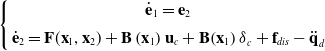 \begin{align} \left\{\begin{array}{c}{\dot{\textbf{e}}}_{1}={\textbf{e}}_{2}\\[5pt] {\dot{\textbf{e}}}_{2}=\textbf{F}({\textbf{x}}_{1},{\textbf{x}}_{2})+\textbf{B}\left({\textbf{x}}_{1}\right){\textbf{u}}_{c}+\textbf{B}{\left({\textbf{x}}_{1}\right){\delta }}_{c}+{\textbf{f}}_{dis}-{\ddot{\textbf{q}}}_{d}\end{array}\right.\end{align}
The main control objective of this paper is to design a tracking control command $ {\textbf{u}}_{c}$
, such that
$ {\textbf{u}}_{c}$
, such that
-
1. All signals in the closed-loop system are bounded.
-
2. Trajectory tracking is fulfilled within a specific time regardless of initial states.
-
3. The position tracking error is always confined within the prescribed performance bounds despite the presence of unknown disturbances, parameter uncertainties and input saturation.
3.0 Controller design and stability analysis
In this section, a continuous adaptive fixed-time sliding mode control method is designed for the free-floating space manipulator system. A novel constraint method based on the prescribed performance function is presented to handle the tracking error constraint issue. Considering the effects of input saturation, an auxiliary compensator is constructed to attain fixed-time stability.
3.1 Non-singular fast terminal slide mode surface
To improve the convergence property, the following non-singularity fast terminal sliding surface (NFTSS) is designed as
 \begin{align} \textbf{s}={\textbf{e}}_{2}+N\left({\textbf{e}}_{1}\right)\left({\textbf{K}}_{1}\textrm{s}\textrm{i}{\textrm{g}}^{1+{\sigma }_{1}}\left({\textbf{e}}_{1}\right)+{\textbf{K}}_{2}{\textbf{s}}_{\rho }\left({\textbf{e}}_{1}\right)\right)\end{align}
where sliding surface $ \textbf{s}=[{s}_{1},{s}_{2}, \ldots ,{s}_{n}{]}^{\textrm{T}}\in {\mathbb{R}}^{n}$
.
$ \textbf{s}=[{s}_{1},{s}_{2}, \ldots ,{s}_{n}{]}^{\textrm{T}}\in {\mathbb{R}}^{n}$
. $ N\left({\textbf{e}}_{1}\right)=1+2{s}_{m}\textrm{a}\textrm{r}\textrm{c}\textrm{t}\textrm{a}\textrm{n}\left({s}_{n}\parallel {\textbf{e}}_{1}{\parallel }^{{s}_{r}}\right)/\pi $
with adjustable positive constants
$ N\left({\textbf{e}}_{1}\right)=1+2{s}_{m}\textrm{a}\textrm{r}\textrm{c}\textrm{t}\textrm{a}\textrm{n}\left({s}_{n}\parallel {\textbf{e}}_{1}{\parallel }^{{s}_{r}}\right)/\pi $
with adjustable positive constants $ {s}_{m}$
,
$ {s}_{m}$
, $ {s}_{n}$
and
$ {s}_{n}$
and $ {s}_{r}$
.
$ {s}_{r}$
. $ {\sigma }_{1}=\frac{{m}_{1}}{2{n}_{1}}(1+\textrm{s}\textrm{g}\textrm{n}(\left|\right|{\textbf{e}}_{1}\left|\right|-1\left)\right)$
with positive odd integers
$ {\sigma }_{1}=\frac{{m}_{1}}{2{n}_{1}}(1+\textrm{s}\textrm{g}\textrm{n}(\left|\right|{\textbf{e}}_{1}\left|\right|-1\left)\right)$
with positive odd integers $ {m}_{1}$
,
$ {m}_{1}$
, $ {n}_{1}$
satisfying
$ {n}_{1}$
satisfying $ {m}_{1}\gt {n}_{1}$
.
$ {m}_{1}\gt {n}_{1}$
. $ {\textbf{K}}_{1}=\textrm{d}\textrm{i}\textrm{a}\textrm{g}({K}_{11},{K}_{12}, \ldots ,{K}_{1n})$
and
$ {\textbf{K}}_{1}=\textrm{d}\textrm{i}\textrm{a}\textrm{g}({K}_{11},{K}_{12}, \ldots ,{K}_{1n})$
and $ {\textbf{K}}_{2}=\textrm{d}\textrm{i}\textrm{a}\textrm{g}({K}_{21},{K}_{22}, \ldots ,{K}_{2n})$
are positive definite matrices.
$ {\textbf{K}}_{2}=\textrm{d}\textrm{i}\textrm{a}\textrm{g}({K}_{21},{K}_{22}, \ldots ,{K}_{2n})$
are positive definite matrices. $ {\textbf{s}}_{\rho }\left({\textbf{e}}_{1}\right)=[{s}_{{\rho }_{1}},{s}_{{\rho }_{2}}, \ldots ,{s}_{{\rho }_{n}}{]}^{\textrm{T}}\in {\mathbb{R}}^{n}$
with
$ {\textbf{s}}_{\rho }\left({\textbf{e}}_{1}\right)=[{s}_{{\rho }_{1}},{s}_{{\rho }_{2}}, \ldots ,{s}_{{\rho }_{n}}{]}^{\textrm{T}}\in {\mathbb{R}}^{n}$
with $ {\textbf{s}}_{{\rho }_{i}}$
is defined as
$ {\textbf{s}}_{{\rho }_{i}}$
is defined as
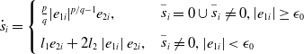
 \begin{align} {s}_{{\rho }_{i}}=\left\{\begin{array}{l@{\quad}l}\textrm{s}\textrm{i}{\textrm{g}}^{p/q}\left({e}_{1i}\right), & {\stackrel{-}{s}}_{i}=0\cup {\stackrel{-}{s}}_{i}\ne 0,\left|{e}_{1i}\right|\ge {\epsilon }_{0}\\[5pt] {l}_{1}{e}_{1i}+{l}_{2}{e}_{1i}^{2}\textrm{s}\textrm{g}\textrm{n}\left({e}_{1i}\right), & {\stackrel{-}{s}}_{i}\ne 0,\left|{e}_{1i}\right| \lt {\epsilon }_{0}\end{array}\right.\end{align}
where $ {\stackrel{-}{s}}_{i}={e}_{2i}+N\left({\textbf{e}}_{1}\right)\left({K}_{1i}\textrm{s}\textrm{i}{\textrm{g}}^{1+{\sigma }_{1}}\left({e}_{1i}\right)+{K}_{2i}\textrm{s}\textrm{i}{\textrm{g}}^{p/q}\left({e}_{1i}\right)\right)$
.
$ {\stackrel{-}{s}}_{i}={e}_{2i}+N\left({\textbf{e}}_{1}\right)\left({K}_{1i}\textrm{s}\textrm{i}{\textrm{g}}^{1+{\sigma }_{1}}\left({e}_{1i}\right)+{K}_{2i}\textrm{s}\textrm{i}{\textrm{g}}^{p/q}\left({e}_{1i}\right)\right)$
. $ p$
,
$ p$
, $ q$
are positive odd integers with
$ q$
are positive odd integers with $ p \lt q$
, and
$ p \lt q$
, and $ {\epsilon }_{0}$
is a small positive constant. To assure the sliding surface and its time derivative smooth and continuous,
$ {\epsilon }_{0}$
is a small positive constant. To assure the sliding surface and its time derivative smooth and continuous, $ {l}_{1}$
and
$ {l}_{1}$
and $ {l}_{2}$
are selected as
$ {l}_{2}$
are selected as
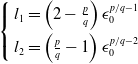 \begin{align} \left\{\begin{array}{ll}{l}_{1}=\left(2-\frac{p}{q}\right){\epsilon }_{0}^{p/q-1} \\[5pt] {l}_{2}=\left(\frac{p}{q}-1\right){\epsilon }_{0}^{p/q-2} \end{array}\right.\end{align}
Lemma 4.
Consider the space manipulator system (12). Once the NFTSS (13) satisfies $ \boldsymbol{s}=0$
, then the system states
$ \boldsymbol{s}=0$
, then the system states $ {\textit{e}}_{1}$
and
$ {\textit{e}}_{1}$
and $ {\textit{e}}_{2}$
convergence to zero along the sliding surface in a fixed time for an arbitrary initial condition. The upper bound of settling time is given by
$ {\textit{e}}_{2}$
convergence to zero along the sliding surface in a fixed time for an arbitrary initial condition. The upper bound of settling time is given by
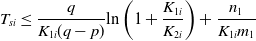
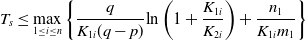 \begin{align} {T}_{s}\le \underset{1\le i\le n}{\textrm{m}\textrm{a}\textrm{x}}\left\{\frac{q}{{K}_{1i}(q-p)}\textrm{l}\textrm{n}\left(1+\frac{{K}_{1i}}{{K}_{2i}}\right)+\frac{{n}_{1}}{{K}_{1i}{m}_{1}}\right\}\end{align}
Proof. Once the MFTSS is reached, i.e., $ \textbf{s}=0$
, a series of the following differential equations can be obtained
$ \textbf{s}=0$
, a series of the following differential equations can be obtained
 \begin{align} {e}_{2i}+N\left({\textbf{e}}_{1}\right)\left({K}_{1i}\textrm{s}\textrm{i}{\textrm{g}}^{1+{\sigma }_{1}}\left({e}_{1i}\right)+{K}_{2i}\textrm{s}\textrm{i}{\textrm{g}}^{p/q}\left({e}_{1i}\right)\right)=0, \quad i=\textrm{1,2}, \ldots ,n\end{align}
Define a new variable as $ Q=|{e}_{1i}{|}^{\frac{q-p}{q}}$
, and the corresponding time-derivative is given by
$ Q=|{e}_{1i}{|}^{\frac{q-p}{q}}$
, and the corresponding time-derivative is given by
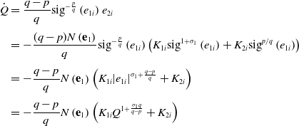 \begin{align} \dot{Q} & =\frac{q-p}{q}\textrm{s}\textrm{i}{\textrm{g}}^{-\frac{p}{q}}\left({e}_{1i}\right){e}_{2i}\nonumber\\[3pt]& =-\frac{(q-p)N\left({\textbf{e}}_{1}\right)}{q}\textrm{s}\textrm{i}{\textrm{g}}^{-\frac{p}{q}}\left({e}_{1i}\right)\left({K}_{1i}\textrm{s}\textrm{i}{\textrm{g}}^{1+{\sigma }_{1}}\left({e}_{1i}\right)+{K}_{2i}\textrm{s}\textrm{i}{\textrm{g}}^{p/q}\left({e}_{1i}\right)\right)\nonumber\\[3pt]& =-\frac{q-p}{q}N\left({\textbf{e}}_{1}\right)\left({K}_{1i}|{e}_{1i}{|}^{{\sigma }_{1}+\frac{q-p}{q}}+{K}_{2i}\right)\\[3pt]& =-\frac{q-p}{q}N\left({\textbf{e}}_{1}\right)\left({K}_{1i}{Q}^{1+\frac{{\sigma }_{1}q}{q-p}}+{K}_{2i}\right)\nonumber\end{align}
According to $ N\left({\textbf{e}}_{1}\right)\ge 1$
, the settling time
$ N\left({\textbf{e}}_{1}\right)\ge 1$
, the settling time $ {T}_{si}$
from
$ {T}_{si}$
from $ {s}_{i}=0$
to
$ {s}_{i}=0$
to $ {e}_{1i}=0$
along the sliding surface is determined by
$ {e}_{1i}=0$
along the sliding surface is determined by
 \begin{align} {T}_{si} & =\frac{q}{(q-p)}{\int }_{0}^{Q(0)} \frac{1}{N\left({\textbf{e}}_{1}\right)\left({K}_{1i}{Q}^{1+\frac{{\sigma }_{1}q}{q-p}}+{K}_{2i}\right)}dQ\nonumber\\[4pt] & =\frac{q}{(q-p)}{\int }_{0}^{1} \frac{1}{N\left({\textbf{e}}_{1}\right)\left({K}_{1i}{Q}^{1+\frac{{\sigma }_{1}q}{q-p}}+{K}_{2i}\right)}dQ\nonumber\\[4pt] &\quad +\frac{q}{(q-p)}{\int }_{1}^{Q(0)} \frac{1}{N\left({\textbf{e}}_{1}\right)\left({K}_{1i}{Q}^{1+\frac{{\sigma }_{1}q}{q-p}}+{K}_{2i}\right)}dQ\nonumber\\[4pt] & =\frac{q}{(q-p)}{\int }_{0}^{1} \frac{1}{N\left({\textbf{e}}_{1}\right)\left({K}_{1i}Q+{K}_{2i}\right)}dQ\\[4pt] &\quad +\frac{q}{(q-p)}{\int }_{1}^{Q(0)} \frac{1}{N\left({\textbf{e}}_{1}\right)\left({K}_{1i}{Q}^{\psi }+{K}_{2i}\right)}dQ\nonumber\\[8pt] & \le \frac{q}{q-p}\left[\frac{1}{{K}_{1i}}\textrm{l}\textrm{n}\left(1+\frac{{K}_{1i}}{{K}_{2i}}\right)+\frac{1-Q(0{)}^{1-\psi }}{{K}_{1i}(\psi -1)}\right]\nonumber \end{align}
where $ \psi =1+\frac{{m}_{1}/{n}_{1}}{1-p/q}$
. Due to
$ \psi =1+\frac{{m}_{1}/{n}_{1}}{1-p/q}$
. Due to $ \psi \gt 1$
and
$ \psi \gt 1$
and $ Q(0)\gt 1$
,
$ Q(0)\gt 1$
, $ {T}_{si}$
is further bounded by
$ {T}_{si}$
is further bounded by
 \begin{align} {T}_{si}\le \frac{q}{{K}_{1i}(q-p)}\textrm{l}\textrm{n}\left(1+\frac{{K}_{1i}}{{K}_{2i}}\right)+\frac{{n}_{1}}{{K}_{1i}{m}_{1}}\end{align}
Based on Equation (20), the upper bound of the convergence time $ {T}_{s}$
can be calculated by
$ {T}_{s}$
can be calculated by
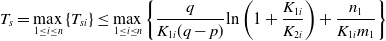 \begin{align} {T}_{s}=\underset{1\le i\le n}{\textrm{m}\textrm{a}\textrm{x}}\left\{{T}_{si}\right\}\le \underset{1\le i\le n}{\textrm{m}\textrm{a}\textrm{x}}\left\{\frac{q}{{K}_{1i}(q-p)}\textrm{l}\textrm{n}\left(1+\frac{{K}_{1i}}{{K}_{2i}}\right)+\frac{{n}_{1}}{{K}_{1i}{m}_{1}}\right\}\end{align}
From Equation (21), the upper bound of convergence time is independent of the system state values. It means that the tracking error $ {\textbf{e}}_{1}$
and its derivative
$ {\textbf{e}}_{1}$
and its derivative $ {\textbf{e}}_{2}$
can converge to the origin within a refined time along the sliding surface. The proof is completed.
$ {\textbf{e}}_{2}$
can converge to the origin within a refined time along the sliding surface. The proof is completed.
Remark 1. It should be pointed out that the strictly positive function $ \textit{N}\left({\textit{e}}_{1}\right)$
in NFTSS (13) is used to tune the convergence rate, which varies from
$ \textit{N}\left({\textit{e}}_{1}\right)$
in NFTSS (13) is used to tune the convergence rate, which varies from $ 1+{s}_{m}$
to
$ 1+{s}_{m}$
to $ 1$
. As the states are far from the origin,
$ 1$
. As the states are far from the origin, $ \textit{N}\left({\textit{e}}_{1}\right)$
approaches
$ \textit{N}\left({\textit{e}}_{1}\right)$
approaches $ 1+{s}_{m}$
that is greater than
$ 1+{s}_{m}$
that is greater than $ 1$
. Once the states are close to the origin,
$ 1$
. Once the states are close to the origin, $ N\left({\textit{e}}_{1}\right)$
tends to
$ N\left({\textit{e}}_{1}\right)$
tends to $ 1$
. The convergence rate is thus improved by introducing
$ 1$
. The convergence rate is thus improved by introducing $ N\left({\textit{e}}_{1}\right)$
. Moreover, a new variable power term
$ N\left({\textit{e}}_{1}\right)$
. Moreover, a new variable power term $ {\sigma }_{1}$
is also included in the NFTSS, which can be adjusted according to the system states. When the states are in the vicinity of the origin, the NFTSS employs a linear term
$ {\sigma }_{1}$
is also included in the NFTSS, which can be adjusted according to the system states. When the states are in the vicinity of the origin, the NFTSS employs a linear term $ {\textit{e}}_{1}$
instead of nonlinear term
$ {\textit{e}}_{1}$
instead of nonlinear term $ si{g}^{\frac{{m}_{1}}{{n}_{1}}}\left({\textit{e}}_{1}\right)$
, which results in a significant increase in the convergence rate. Therefore, the proposed NFTSS exhibits a superior convergence performance whether far from or within a small allowable range of the origin.
$ si{g}^{\frac{{m}_{1}}{{n}_{1}}}\left({\textit{e}}_{1}\right)$
, which results in a significant increase in the convergence rate. Therefore, the proposed NFTSS exhibits a superior convergence performance whether far from or within a small allowable range of the origin.
Remark 2. Huang et al. [Reference Huang and Jia40] presented a fixed-time sliding surface $ \boldsymbol{s}={\textit{e}}_{2}+{\textit{K}}_{1}si{g}^{{m}_{1}/{n}_{1}}\left({\textit{e}}_{1}\right)+{\textit{K}}_{2}{\boldsymbol{s}}_{\rho }\left({\textit{e}}_{1}\right)$
with
$ \boldsymbol{s}={\textit{e}}_{2}+{\textit{K}}_{1}si{g}^{{m}_{1}/{n}_{1}}\left({\textit{e}}_{1}\right)+{\textit{K}}_{2}{\boldsymbol{s}}_{\rho }\left({\textit{e}}_{1}\right)$
with $ {\stackrel{-}{s}}_{i}={e}_{2i}+{K}_{1i}si{g}^{{m}_{1}/{n}_{1}}\left({e}_{1i}\right)+{K}_{2i}si{g}^{p/q}\left({e}_{1i}\right)$
, and derived the upper bound of convergence time
$ {\stackrel{-}{s}}_{i}={e}_{2i}+{K}_{1i}si{g}^{{m}_{1}/{n}_{1}}\left({e}_{1i}\right)+{K}_{2i}si{g}^{p/q}\left({e}_{1i}\right)$
, and derived the upper bound of convergence time $ {T}_{1}={max}_{1\le i\le n}\left\{\frac{q}{{K}_{2i}(q-p)}+\frac{{n}_{1}}{{K}_{1i}\left({m}_{1}-{n}_{1}\right)}\right\}$
. Another fast fixed-time sliding surface
$ {T}_{1}={max}_{1\le i\le n}\left\{\frac{q}{{K}_{2i}(q-p)}+\frac{{n}_{1}}{{K}_{1i}\left({m}_{1}-{n}_{1}\right)}\right\}$
. Another fast fixed-time sliding surface $ \boldsymbol{s}={\textit{e}}_{2}+{\textit{K}}_{1}{\textit{e}}_{1}^{\frac{1}{2}+\frac{m1}{2n1}+(\frac{m1}{2n1}-\frac{1}{2})sgn\left(\right|{\textit{e}}_{1}|-1)}$ $ +{\textit{K}}_{2}{\textit{e}}_{1}^{\frac{p}{q}}$
is investigated in Ref. [Reference Ni, Liu, Liu, Hu and Li41] and the settling time upper-bound was given by
$ +{\textit{K}}_{2}{\textit{e}}_{1}^{\frac{p}{q}}$
is investigated in Ref. [Reference Ni, Liu, Liu, Hu and Li41] and the settling time upper-bound was given by $ {T}_{2}={max}_{1\le i\le n}\left\{\frac{q}{{K}_{1i}(q-p)}ln\left(1+\frac{{K}_{1i}}{{K}_{2i}}\right)+\frac{{n}_{1}}{{K}_{1i}({m}_{1}-{n}_{1})}\right\}$
. Since the relation
$ {T}_{2}={max}_{1\le i\le n}\left\{\frac{q}{{K}_{1i}(q-p)}ln\left(1+\frac{{K}_{1i}}{{K}_{2i}}\right)+\frac{{n}_{1}}{{K}_{1i}({m}_{1}-{n}_{1})}\right\}$
. Since the relation $ ln\left(1+{K}_{1i}/{K}_{2i}\right) \lt {K}_{1i}/{K}_{2i}$
holds, one has
$ ln\left(1+{K}_{1i}/{K}_{2i}\right) \lt {K}_{1i}/{K}_{2i}$
holds, one has $ {T}_{s} \lt {T}_{2} \lt {T}_{1}$
, which implies that under the same design parameters, the proposed NFTSS obtains the fastest convergence rate.
$ {T}_{s} \lt {T}_{2} \lt {T}_{1}$
, which implies that under the same design parameters, the proposed NFTSS obtains the fastest convergence rate.
3.2 Prescribed performance function
Appropriate constraints on the system states are necessary to obtain the desired dynamic performance. With this in mind, the PPC is investigated to confine the position tracking error within a predefined permissible range here. First, describe such a constraint via a prescribed performance function, defined as follows.
Definition 2. [Reference Bechlioulis and Rovithakis26] if a positive continuous function $ \rho (t)$
satisfies 1)
$ \rho (t)$
satisfies 1) $ \rho (t)\gt 0$
and
$ \rho (t)\gt 0$
and $ \dot{\rho }(t)\le 0$
2)
$ \dot{\rho }(t)\le 0$
2) $ {lim}_{t\to \infty }\rho (t)={\rho }_{\infty }\gt 0$
, then
$ {lim}_{t\to \infty }\rho (t)={\rho }_{\infty }\gt 0$
, then $ \rho (t)$
is called a performance function.
$ \rho (t)$
is called a performance function.
Generally, a prescribed performance function is designed as
 \begin{align} \rho (t)=\left({\rho }_{0}-{\rho }_{{\infty }}\right){\textrm{e}}^{-{l}_{0}t}+{\rho }_{{\infty }}\end{align}
where $ {\rho }_{0}\gt {\rho }_{{\infty }}\gt 0$
and
$ {\rho }_{0}\gt {\rho }_{{\infty }}\gt 0$
and $ {l}_{0}\gt 0$
are design parameters and should be set appropriately to obtain the desired time-domain characteristics, such as steady-state offset, overshoot and rising time. As stated in Ref. [Reference Ik Han and Lee46], the prescribed performance is attained provided that the state is limited to the area bounded by the decaying function of time. According to the concept, achieving the prescribed error constraints is equivalent to satisfy the following relationship:
$ {l}_{0}\gt 0$
are design parameters and should be set appropriately to obtain the desired time-domain characteristics, such as steady-state offset, overshoot and rising time. As stated in Ref. [Reference Ik Han and Lee46], the prescribed performance is attained provided that the state is limited to the area bounded by the decaying function of time. According to the concept, achieving the prescribed error constraints is equivalent to satisfy the following relationship:
 \begin{align} -{\rho }_{i}(t) \lt {e}_{1i}(t) \lt {\rho }_{i}(t)\end{align}
where $ {\rho }_{i}$
denotes the prescribed performance function of
$ {\rho }_{i}$
denotes the prescribed performance function of $ {s}_{i}$
.
$ {s}_{i}$
.
Based on the condition (23), one concludes that as long as $ \left|{e}_{1i}(0)\right| \lt {\rho }_{i}(0)$
is satisfied, the tracking error is always never exceed the predefined boundary.
$ \left|{e}_{1i}(0)\right| \lt {\rho }_{i}(0)$
is satisfied, the tracking error is always never exceed the predefined boundary.
Remark 3.
Define transformed constraint error $ {z}_{i}$
as
$ {z}_{i}$
as $ {z}_{i}={e}_{1i}/{\rho }_{i}$
. Obviously, when the constraint (23) is satisfied,
$ {z}_{i}={e}_{1i}/{\rho }_{i}$
. Obviously, when the constraint (23) is satisfied, $ {z}_{i}$
becomes
$ {z}_{i}$
becomes $ {z}_{i}\in ({-}\textrm{1,1})$
. That is, when
$ {z}_{i}\in ({-}\textrm{1,1})$
. That is, when $ \left|{e}_{1i}(t)\right|$
tends to the boundary
$ \left|{e}_{1i}(t)\right|$
tends to the boundary $ {\rho }_{i}(t)$
,
$ {\rho }_{i}(t)$
, $ {z}_{i}$
approaches
$ {z}_{i}$
approaches $ 1$
.
$ 1$
.
3.3 Fixed-time tracking controller design
Take the time derivative of $ \textbf{s}$
in Equation (13) and using Equation (12), one obtains
$ \textbf{s}$
in Equation (13) and using Equation (12), one obtains
 \begin{align} \dot{\textbf{s}} & =\textbf{F}({\textbf{x}}_{1},{\textbf{x}}_{2})+\textbf{B}\left({\textbf{x}}_{1}\right){\textbf{u}}_{c}+\textbf{B}{\left({\textbf{x}}_{1}\right){\delta }}_{c}+{\textbf{f}}_{dis}-{\ddot{\textbf{q}}}_{d}\nonumber\\[4pt] & \quad +\dot{N}\left({\textbf{e}}_{1}\right)\left({\textbf{K}}_{1}\textrm{s}\textrm{i}{\textrm{g}}^{1+{\sigma }_{1}}\left({\textbf{e}}_{1}\right)+{\textbf{K}}_{2}{\textbf{s}}_{\rho }\left({\textbf{e}}_{1}\right)\right)\\[4pt] & \quad +N\left({\textbf{e}}_{1}\right)\left((1+{\sigma }_{1}){\textbf{K}}_{1}\textrm{d}\textrm{i}\textrm{a}\textrm{g}\left(\right|{e}_{1i}{|}^{{\sigma }_{1}}){\textbf{e}}_{2}+{\textbf{K}}_{2}{\dot{\textbf{s}}}_{\rho }({\textbf{e}}_{1})\right)\nonumber\end{align}
where the $ i$
th element of
$ i$
th element of $ {\dot{\textbf{s}}}_{\rho }$
is given by
$ {\dot{\textbf{s}}}_{\rho }$
is given by
 \begin{align} {\dot{s}}_{i}=\left\{\begin{array}{l@{\quad}l}\frac{p}{q}|{e}_{1i}{|}^{p/q-1}{e}_{2i}, & {\stackrel{-}{s}}_{i}=0\cup {\stackrel{-}{s}}_{i}\ne 0,\left|{e}_{1i}\right|\ge {\epsilon }_{0}\\[5pt] {l}_{1}{e}_{2i}+2{l}_{2}\left|{e}_{1i}\right|{e}_{2i}, & {\stackrel{-}{s}}_{i}\ne 0,\left|{e}_{1i}\right| \lt {\epsilon }_{0}\end{array}\right.\end{align}
Aiming to attain trajectory tracking with high precision, the following adaptive nonsingular fixed-time sliding mode control with prescribed performance constraints is developed
 \begin{align} {\textbf{u}}_{c}={\textbf{u}}_{eq}+{\textbf{u}}_{r}+{\textbf{u}}_{s}\end{align}
where,
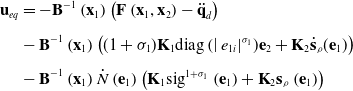 \begin{align} {\textbf{u}}_{eq} & = -{\textbf{B}}^{-1}\left({\textbf{x}}_{1}\right)\left(\textbf{F}\left({\textbf{x}}_{1},{\textbf{x}}_{2}\right)-{\ddot{\textbf{q}}}_{d}\right)\nonumber\\[5pt] & -{\textbf{B}}^{-1}\left({\textbf{x}}_{1}\right)\left((1+{\sigma }_{1}){\textbf{K}}_{1}\textrm{d}\textrm{i}\textrm{a}\textrm{g}\left(\right|{e}_{1i}{|}^{{\sigma }_{1}}){\textbf{e}}_{2}+{\textbf{K}}_{2}{\dot{\textbf{s}}}_{\rho }({\textbf{e}}_{1})\right)\\[5pt] & -{\textbf{B}}^{-1}\left({\textbf{x}}_{1}\right)\dot{N}\left({\textbf{e}}_{1}\right)\left({\textbf{K}}_{1}\textrm{s}\textrm{i}{\textrm{g}}^{1+{\sigma }_{1}}\left({\textbf{e}}_{1}\right)+{\textbf{K}}_{2}{\textbf{s}}_{\rho }\left({\textbf{e}}_{1}\right)\right)\qquad\quad\nonumber \end{align}
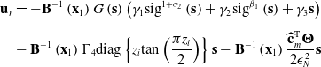 \begin{align} {\textbf{u}}_{r} & = -{\textbf{B}}^{-1}\left({\textbf{x}}_{1}\right)G\left(\textbf{s}\right)\left({\gamma }_{1}\textrm{s}\textrm{i}{\textrm{g}}^{1+{\sigma }_{2}}\left(\textbf{s}\right)+{\gamma }_{2}\textrm{s}\textrm{i}{\textrm{g}}^{{\beta }_{1}}\left(\textbf{s}\right)+{\gamma }_{3}\textbf{s}\right)\nonumber\\[5pt] & -{\textbf{B}}^{-1}\left({\textbf{x}}_{1}\right){{\Gamma }}_{4}\textrm{d}\textrm{i}\textrm{a}\textrm{g}\left\{{z}_{i}\textrm{t}\textrm{a}\textrm{n}\left(\frac{\pi {z}_{i}}{2}\right)\right\}\textbf{s}-{\textbf{B}}^{-1}\left({\textbf{x}}_{1}\right)\frac{{\widehat{\textbf{c}}}_{m}^{\textrm{T}}{\boldsymbol\Theta }}{2{\epsilon }_{N}^{2}}\textbf{s} \end{align}
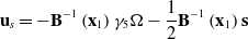 \begin{align} {\textbf{u}}_{s}=-{\textbf{B}}^{-1}\left({\textbf{x}}_{1}\right){\gamma }_{5}{\Omega }-\frac{1}{2}{\textbf{B}}^{-1}\left({\textbf{x}}_{1}\right)\textbf{s}\qquad\qquad\qquad\qquad\end{align}
 \begin{align} G\left(s\right)=1+\chi -\chi {\textrm{e}}^{-{v}_{1}\left|\right|\textbf{s}|{|}^{k}}\qquad\qquad\qquad\qquad\quad\end{align}
where $ {\sigma }_{2}=\frac{{\alpha }_{1}}{2}\left(1+\textrm{s}\textrm{g}\textrm{n}\left(\right|\left|\textbf{s}\right||-1)\right)$
with
$ {\sigma }_{2}=\frac{{\alpha }_{1}}{2}\left(1+\textrm{s}\textrm{g}\textrm{n}\left(\right|\left|\textbf{s}\right||-1)\right)$
with $ {\alpha }_{1}\gt 1$
, and
$ {\alpha }_{1}\gt 1$
, and $ {\beta }_{1}\in \left(\textrm{0,1}\right)$
.
$ {\beta }_{1}\in \left(\textrm{0,1}\right)$
. $ \chi \gt 0$
,
$ \chi \gt 0$
, $ {v}_{1}\gt 0$
and
$ {v}_{1}\gt 0$
and $ k$
is a positive integer,
$ k$
is a positive integer, $ {\gamma }_{1},{\gamma }_{2},{\gamma }_{3},{\gamma }_{5}$
are positive design parameters,
$ {\gamma }_{1},{\gamma }_{2},{\gamma }_{3},{\gamma }_{5}$
are positive design parameters, $ {{\Gamma }}_{4}=\textrm{d}\textrm{i}\textrm{a}\textrm{g}\left({\gamma }_{41},{\gamma }_{42}, \ldots ,{\gamma }_{4n}\right)$
is a positive constant matrix, which is used as the tuning gain to force the tracking error to remain within the defined boundary.
$ {{\Gamma }}_{4}=\textrm{d}\textrm{i}\textrm{a}\textrm{g}\left({\gamma }_{41},{\gamma }_{42}, \ldots ,{\gamma }_{4n}\right)$
is a positive constant matrix, which is used as the tuning gain to force the tracking error to remain within the defined boundary. $ {\widehat{\textbf{c}}}_{m}$
is the estimation of
$ {\widehat{\textbf{c}}}_{m}$
is the estimation of $ {\textbf{c}}_{m}$
with
$ {\textbf{c}}_{m}$
with $ {\textbf{c}}_{m}={\left[{c}_{1}^{2},{c}_{2}^{2},{c}_{3}^{2}\right]}^{\textrm{T}}$
, and
$ {\textbf{c}}_{m}={\left[{c}_{1}^{2},{c}_{2}^{2},{c}_{3}^{2}\right]}^{\textrm{T}}$
, and $ {\boldsymbol\Theta }={\left[1,\parallel {\textbf{x}}_{1}{\parallel }^{2},\parallel {\textbf{x}}_{2}{\parallel }^{4}\right]}^{\textrm{T}}$
. The adaptive update law is designed as
$ {\boldsymbol\Theta }={\left[1,\parallel {\textbf{x}}_{1}{\parallel }^{2},\parallel {\textbf{x}}_{2}{\parallel }^{4}\right]}^{\textrm{T}}$
. The adaptive update law is designed as
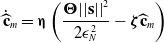 \begin{align} {\dot{\widehat{\textbf{c}}}}_{m}={\boldsymbol\eta}\left(\frac{{{\boldsymbol\Theta}||\textbf{s}||}^{2}}{2{\epsilon }_{N}^{2}}-\boldsymbol{\zeta}{\widehat{\textbf{c}}}_{m}\right)\end{align}
where $ \boldsymbol{\eta} =\textrm{d}\textrm{i}\textrm{a}\textrm{g}({\eta }_{1},{\eta }_{2},{\eta }_{3})$
and
$ \boldsymbol{\eta} =\textrm{d}\textrm{i}\textrm{a}\textrm{g}({\eta }_{1},{\eta }_{2},{\eta }_{3})$
and $ \boldsymbol{\zeta} =\textrm{d}\textrm{i}\textrm{a}\textrm{g}({\zeta }_{1},{\zeta }_{2},{\zeta }_{3})$
are two positive matrices, and
$ \boldsymbol{\zeta} =\textrm{d}\textrm{i}\textrm{a}\textrm{g}({\zeta }_{1},{\zeta }_{2},{\zeta }_{3})$
are two positive matrices, and $ {\epsilon }_{N}$
is an arbitrary small positive constant.
$ {\epsilon }_{N}$
is an arbitrary small positive constant.
To compensate for input saturation, the auxiliary variable $ {\boldsymbol\Omega }$
is given by
$ {\boldsymbol\Omega }$
is given by
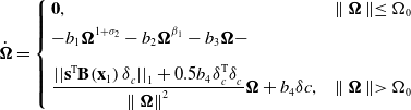 \begin{align} \dot{{\boldsymbol\Omega }}=\left\{\begin{array}{l@{\quad}l}\boldsymbol{0}, & \parallel {\boldsymbol\Omega }\parallel \le {{\Omega }}_{0}\\[4pt] -{b}_{1}{{\boldsymbol\Omega }}^{1+{\sigma }_{2}}-{b}_{2}{{\boldsymbol\Omega }}^{{\beta }_{1}}-{b}_{3}{\boldsymbol\Omega }- & \\[8pt] \dfrac{{||{\textbf{s}}^{\textrm{T}}\textbf{B}{\left({\textbf{x}}_{1}\right){\delta }}_{c}||}_{1}+0.5{{{b}_{4}{\delta }}_{c}^{\textrm{T}}{\delta }}_{c}}{\parallel {\boldsymbol\Omega }{\parallel }^{2}}{\boldsymbol\Omega }+{{b}_{4}} {{\delta }c}, & \parallel {\boldsymbol\Omega }\parallel \gt {{\Omega }}_{0}\end{array}\right.\end{align}
where $ {b}_{1},{b}_{2},{b}_{3},{b}_{4}$
and
$ {b}_{1},{b}_{2},{b}_{3},{b}_{4}$
and $ {{\Omega }}_{0}$
are positive constants.
$ {{\Omega }}_{0}$
are positive constants.
Remark 4. The auxiliary variable combined with fast terminal sliding mode control enables fixed-time convergence of tracking control. The parameter $ {b}_{4}$
is intended to avoid the possible overcompensation of actuator saturation.
$ {b}_{4}$
is intended to avoid the possible overcompensation of actuator saturation.
Remark 5. It is worth noting that when $ \left|{e}_{1i}\right|$
approaches the constraint boundary
$ \left|{e}_{1i}\right|$
approaches the constraint boundary $ {\rho }_{i}$
, then
$ {\rho }_{i}$
, then $ {z}_{i}\to 1$
, and the value of
$ {z}_{i}\to 1$
, and the value of $ tan\left(\frac{\pi {z}_{i}}{2}\right)$
tends to infinity. The control gain is thus increased to suppress the evolution of the tracking error. Figure 2 illustrates this constraint control scheme in graphical form. If the required control law is unreasonable or the evolution of tracking error violates the constraint boundaries, the values of
$ tan\left(\frac{\pi {z}_{i}}{2}\right)$
tends to infinity. The control gain is thus increased to suppress the evolution of the tracking error. Figure 2 illustrates this constraint control scheme in graphical form. If the required control law is unreasonable or the evolution of tracking error violates the constraint boundaries, the values of $ {\rho }_{0}$
,
$ {\rho }_{0}$
, $ {\rho }_{\infty }$
,
$ {\rho }_{\infty }$
, $ {l}_{0}$
and
$ {l}_{0}$
and $ {{\Gamma }}_{4}$
must be adjusted according to practical application.
$ {{\Gamma }}_{4}$
must be adjusted according to practical application.
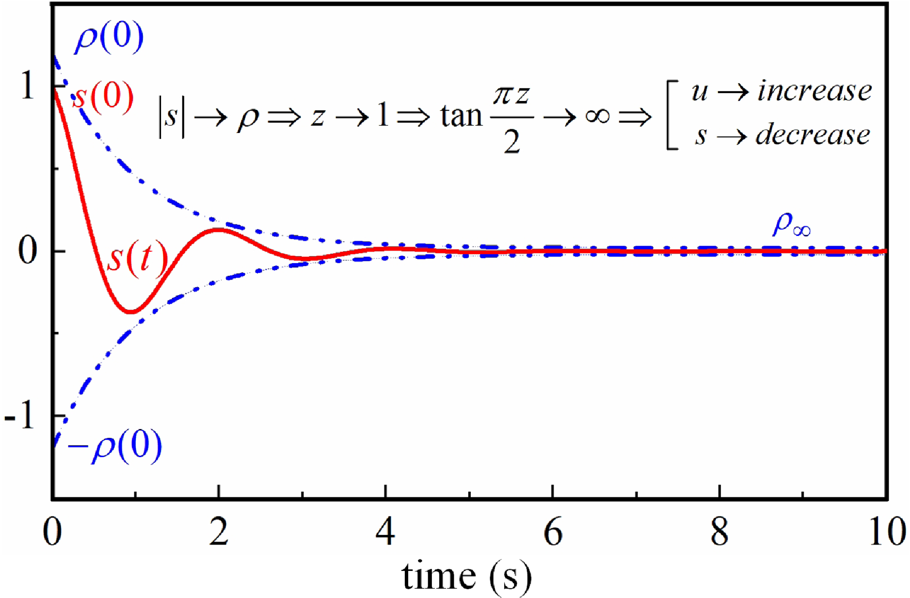
Figure 2. The description of the constraint control scheme.
Lemma 5.
Consider the space manipulator system (12) with the lumped uncertainty satisfying Assumption 2. If the sliding surface is defined as Equation (13) and the control laws are designed as Equations (26)–(30) with the adaptive update law Equation (31) and the auxiliary system Equation (32), then the system trajectory enables to enforce into the vicinity of the sliding surface $ \boldsymbol{s}=0$
from any initial states within a fixed time. Furthermore, system’s tracking errors
$ \boldsymbol{s}=0$
from any initial states within a fixed time. Furthermore, system’s tracking errors $ {\textit{e}}_{1}$
and
$ {\textit{e}}_{1}$
and $ {\textit{e}}_{2}$
converge to a small set containing the region.
$ {\textit{e}}_{2}$
converge to a small set containing the region.
For a deeper understanding of the overall structure of the suggested method, Fig. 3 shows the closed-loop tracking control system.
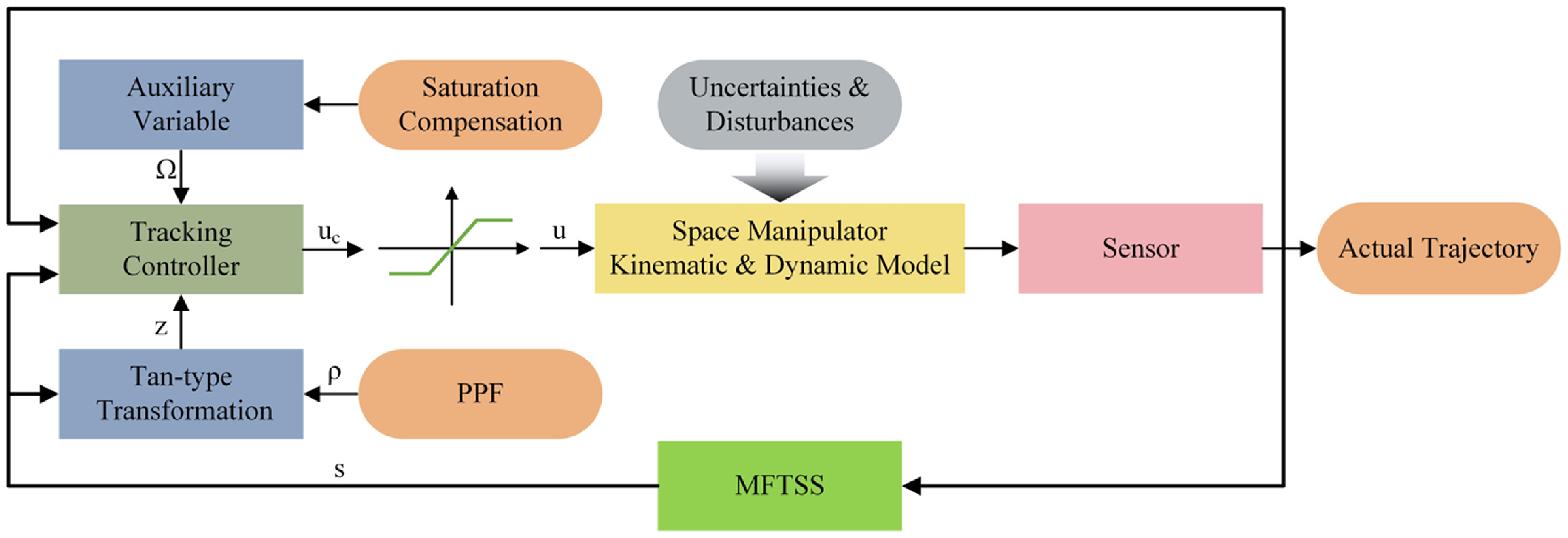
Figure 3. The structure of the proposed control scheme.
3.4 Stability analysis
To prove Lemma 5, the following will analyse and demonstrate in two steps.
-
Step 1. Fixed time convergence property of the sliding surface
$ \boldsymbol{s}$
is verified.

Substituting Equations (26)–(29) into Equation (24), one obtains
 \begin{align} \dot{\textbf{s}} & =-G\left(\textbf{s}\right)\left({\gamma }_{1}\textrm{s}\textrm{i}{\textrm{g}}^{1+{\sigma }_{2}}\left(\textbf{s}\right)+{\gamma }_{2}\textrm{s}\textrm{i}{\textrm{g}}^{{\beta }_{1}}\left(\textbf{s}\right)+{\gamma }_{3}\textbf{s}\right)+\textbf{B}{\left({\textbf{x}}_{1}\right){\delta }}_{c}\nonumber\\[5pt]& -{{\Gamma }}_{4}\textrm{d}\textrm{i}\textrm{a}\textrm{g}\left\{{z}_{i}\textrm{t}\textrm{a}\textrm{n}\left(\frac{\pi {z}_{i}}{2}\right)\right\}\textbf{s}-\left(\frac{{\widehat{\textbf{c}}}_{m}^{\textrm{T}}{\Theta }}{2{\epsilon }_{N}^{2}}+\frac{1}{2}\right)\textbf{s}-{\gamma }_{5}{\Omega }+{\textbf{f}}_{dis} \end{align}
To validate the stability of the closed-loop system, define the following Lyapunov function:
 \begin{align} {V}_{2}=\frac{1}{2}{\textbf{s}}^{\textrm{T}}\textbf{s}+\frac{1}{2}{{\tilde{\textbf{c}}}_{m}^{\textrm{T}}} \boldsymbol{\eta}^{-1}{\tilde{\textbf{c}}}_{m}+\frac{1}{2}{{\Omega }}^{\textrm{T}}{\Omega }\end{align}
where $ \tilde{\textbf{c}}_{m}={\textbf{c}}_{m}-{\widehat{\textbf{c}}}_{m}$
denotes the estimate error of
$ \tilde{\textbf{c}}_{m}={\textbf{c}}_{m}-{\widehat{\textbf{c}}}_{m}$
denotes the estimate error of $ {\textbf{c}}_{m}$
.
$ {\textbf{c}}_{m}$
.
The derivative of $ {V}_{2}$
with respect to time yields
$ {V}_{2}$
with respect to time yields
 \begin{align} \dot{{V}}_{2}=\textbf{s}^{\text{T}} \dot{\textbf{s}} - \tilde{\textbf{c}}_{m}^{\text{T}} \boldsymbol{\eta}^{-1} \dot{\hat{\textbf{c}}}_{m} +\boldsymbol{\Omega}^{\text{T}} \dot{\boldsymbol{\Omega}}\end{align}
Then, one can derive
 \begin{align} \dot{V}_{2}=&-\textbf{s}^{\text{T}}\left\{G \left(\textbf{s}\right) \left(\gamma_{1}{\textrm{sig}}^{1+\sigma_2}(\textbf{s}) + \gamma_{2} {\textrm{sig}}^{\beta_1}(\textbf{s}) + \gamma_{3} \textbf{s}\right)-\textbf{B}\left(\textbf{x}_{1}\right)\boldsymbol{\delta}_{c}\right. \nonumber\\ & \left.+ \boldsymbol{\Gamma_{4}} \textrm{diag}\left\{ z_{i} \tan\left(\frac{\pi z_{i}}{2}\right) \right\} \textbf{s} +\left(\frac{\hat{\textbf{c}}_{m}^{\text{T}} \boldsymbol{\Theta}}{2 \varepsilon_N^{2}} + \frac{1}{2}\right) \textbf{s}+\gamma_{5}\boldsymbol{\Omega}-\textbf{f}_{dis}\right\}\nonumber\\ &- \tilde{\textbf{c}}_{m}^{\text{T}} \left( \frac{\boldsymbol{\Theta}\left\|{\textbf{s}}\right\|^{2}}{2 \varepsilon_N^{2}}-\boldsymbol{\zeta} \hat{\textbf{c}}_{m} \right) +\boldsymbol{\Omega}^{\text{T}} \dot{\boldsymbol{\Omega}}\nonumber\\ =& - G \left(\textbf{s}\right) \left(\gamma_{1}\|\textbf{s}\|^{\sigma_2+2}+ \gamma_{2}\|\textbf{s}\|^{\beta_1+1}+ \gamma_{3}\|\textbf{s}\|^{2}\right)\\ & - \textbf{s}^{\text{T}} \boldsymbol{\Gamma_{4}} \textrm{diag}\left\{ z_{i} \tan\left(\frac{\pi z_{i}}{2}\right) \right\} \textbf{s} - \frac{\hat{\textbf{c}}_{m}^{\text{T}} \boldsymbol{\Theta}}{2 \varepsilon_N^{2}}\|\textbf{s}\|^{2} + \textbf{s}^{\text{T}} \textbf{f}_{dis} -\frac{\tilde{\textbf{c}}_{m}^{\text{T}}\boldsymbol{\Theta}}{2\varepsilon_N^{2}}\left\|{\textbf{s}}\right\|^{2} \nonumber\\ & + \tilde{\textbf{c}}_{m}^{\text{T}} \boldsymbol{\zeta} \hat{\textbf{c}}_{m} -\frac{1}{2}\textbf{s}^{\text{T}}\textbf{s} -\gamma_{5}\textbf{s}^{\text{T}}\boldsymbol{\Omega}+\textbf{s}^{\text{T}}\textbf{B}\left(\textbf{x}_1\right)\boldsymbol{\delta}_{c}+\boldsymbol{\Omega}^{\text{T}}\dot{\boldsymbol{\Omega}}\nonumber \end{align}
Considering the auxiliary system Equation (32), the above equation leads to
 \begin{align} \dot{V}_{2}=& - G \left(\textbf{s}\right) \left(\gamma_{1}\|\textbf{s}\|^{\sigma_2+2}+ \gamma_{2}\|\textbf{s}\|^{\beta_1+1}+ \gamma_{3}\|\textbf{s}\|^{2}\right)\nonumber\\[5pt] & - \textbf{s}^{\text{T}}\boldsymbol{\Gamma_{4}} \textrm{diag} \left\{ z_{i} \tan\left(\frac{\pi z_{i}}{2}\right)\right\} \textbf{s} - \frac{\hat{\textbf{c}}_{m}^{\text{T}} \boldsymbol{\Theta}}{2 \varepsilon_N^{2}}\| \textbf{s}\|^{2} + \textbf{s}^{\text{T}} \textbf{f}_{dis} -\frac{\tilde{\textbf{c}}_{m}^{\text{T}}\boldsymbol{\Theta}}{2\varepsilon_N^{2}}\left\|{\textbf{s}}\right\|^{2} \nonumber\\[5pt] & + \tilde{\textbf{c}}_{m}^{\text{T}} \boldsymbol{\zeta} \hat{\textbf{c}}_{m} -\frac{1}{2}\textbf{s}^{\text{T}}\textbf{s} -\gamma_{5}\textbf{s}^{\text{T}}\boldsymbol{\Omega}+\textbf{s}^{\text{T}}\textbf{B}\left(\textbf{x}_1\right)\boldsymbol{\delta}_{c} -b_{1}\boldsymbol{\Omega}^{\text{T}}\boldsymbol{\Omega}^{1+\sigma_{2}}\nonumber\\[5pt] & -b_{2}\boldsymbol{\Omega}^{\text{T}}\boldsymbol{\Omega}^{\beta_{1}} -b_{3}\boldsymbol{\Omega}^{\text{T}}\boldsymbol{\Omega} -\left\|\textbf{s}^{\text{T}} \textbf{B}\left(\textbf{x}_{1}\right) \boldsymbol{\delta}_{c}\right\|_{1} -\frac{1}{2} b_{4} \boldsymbol{\delta}_{c}^{\text{T}} \boldsymbol{\delta}_{c} +b_{4}\boldsymbol{\Omega}^{\text{T}}\boldsymbol{\delta}_{c}\nonumber\\[5pt] \leq & - G \left(\textbf{s}\right) \left(\gamma_{1}\|\textbf{s}\|^{\sigma_2+2}+ \gamma_{2}\|\textbf{s}\|^{\beta_1+1}+ \gamma_{3}\|\textbf{s}\|^{2}\right)\\[5pt] & - \boldsymbol{\Gamma_{4}} \textrm{diag} \left\{z_{i}\tan\left(\frac{\pi z_{i}}{2}\right)\right\} \|\textbf{s}\|^2 - \frac{{\textbf{c}}_{m}^{\text{T}} \boldsymbol{\Theta}}{2 \varepsilon_N^{2}}\|\textbf{s}\|^{2} + \textbf{c}_{z}^{\text{T}}\boldsymbol{theta}\|\textbf{s}\| +\tilde{\textbf{c}}_{m}^{\text{T}}\boldsymbol{ \zeta }\hat{\textbf{c}}_{m}\nonumber\\[5pt] & -\frac{1}{2}\textbf{s}^{\text{T}}\textbf{s} -\gamma_{5}\textbf{s}^{\text{T}}\boldsymbol{\Omega} -b_{1}\boldsymbol{\Omega}^{\text{T}}\boldsymbol{\Omega}^{1+\sigma_2}-b_{2}\boldsymbol{\Omega}^{\text{T}}\boldsymbol{\Omega}^{\beta_{1}} -b_{3}\boldsymbol{\Omega}^{\text{T}}\boldsymbol{\Omega}\nonumber\\[5pt] & -\frac{1}{2} b_{4} \boldsymbol{\delta}_{c}^{\text{T}} \boldsymbol{\delta}_{c} +b_{4}\boldsymbol{\Omega}^{\text{T}}\boldsymbol{\delta}_{c}\nonumber \end{align}
According to Young’s inequality, for $ \forall {\lambda }_{j}\gt \frac{1}{2}$
,
$ \forall {\lambda }_{j}\gt \frac{1}{2}$
, $ j=(\textrm{1,2},3)$
, the following inequality relations hold:
$ j=(\textrm{1,2},3)$
, the following inequality relations hold:
 \begin{align} \textbf{c}_{z}^{\text{T}}\boldsymbol{theta}\|\textbf{s}\|=c_1\|\textbf{s}\|+c_2\|\textbf{x}_1\|\|\textbf{s}\|+c_3\|\textbf{x}_2\|^2\|\textbf{s}\| \leq \frac{\textbf{c}_{m}^{\text{T}}\boldsymbol{\Theta}}{2\varepsilon_N^{2}}\|\textbf{s}\|^{2} +\frac{3}{2}\varepsilon_{N}^{2}\end{align}
 \begin{align} \tilde{\textbf{c}}_{m}^{\text{T}}\boldsymbol{\zeta}\hat{\textbf{c}}_{m}&=\sum_{j=1}^{3}\zeta_j\tilde{c}_{m_j}\hat{c}_{m_j}=\sum_{j=1}^{3}\zeta_j\tilde{c}_{m_j}\left(c_{m_j}-\tilde{c}_{m_j} \right)\nonumber\\ & \leq\sum_{j=1}^{3}\zeta_j\left(\frac{\lambda_{j}}{2}c_{m_j}^{2} -\frac{2\lambda_{j}-1}{2\lambda_{j}}\tilde{c}_{m_j}^{2} \right)\end{align}
 \begin{align} -\gamma_{5}\textbf{s}^{\text{T}}\boldsymbol{\Omega}\leq\frac{1}{2}\textbf{s}^{\text{T}}\textbf{s}+\frac{1}{2}\gamma_{5}^{2}\boldsymbol{\Omega}^{\text{T}}\boldsymbol{\Omega}\end{align}
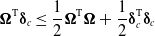 \begin{align} \boldsymbol{\Omega}^{\text{T}}\boldsymbol{\delta}_{c}\leq\frac{1}{2}\boldsymbol{\Omega}^{\text{T}}\boldsymbol{\Omega}+\frac{1}{2}\boldsymbol{\delta}_{c}^{\text{T}}\boldsymbol{\delta}_{c}\end{align}
Remark 6. For $ {z}_{i}={e}_{1i}/{\rho }_{i}$
, when
$ {z}_{i}={e}_{1i}/{\rho }_{i}$
, when $ {e}_{1i} \lt 0$
,
$ {e}_{1i} \lt 0$
, $ {z}_{i} \lt 0$
holds and then
$ {z}_{i} \lt 0$
holds and then $ tan\left(\frac{\pi {z}_{i}}{2}\right) \lt 0$
, resulting in
$ tan\left(\frac{\pi {z}_{i}}{2}\right) \lt 0$
, resulting in $ {z}_{i}tan\left(\frac{\pi {z}_{i}}{2}\right)\gt 0$
. Similarly, when
$ {z}_{i}tan\left(\frac{\pi {z}_{i}}{2}\right)\gt 0$
. Similarly, when $ {e}_{1i}\ge 0$
,
$ {e}_{1i}\ge 0$
, $ {z}_{i}\ge 0$
holds and then
$ {z}_{i}\ge 0$
holds and then $ tan\left(\frac{\pi {z}_{i}}{2}\right)\ge 0$
, leading to
$ tan\left(\frac{\pi {z}_{i}}{2}\right)\ge 0$
, leading to $ {z}_{i}tan\left(\frac{\pi {z}_{i}}{2}\right)\ge 0$
. In summary,
$ {z}_{i}tan\left(\frac{\pi {z}_{i}}{2}\right)\ge 0$
. In summary, $ {z}_{i}tan\left(\frac{\pi {z}_{i}}{2}\right)$
is consistently non-negative.
$ {z}_{i}tan\left(\frac{\pi {z}_{i}}{2}\right)$
is consistently non-negative.
Using the above inequalities, Equation (37) can be written as
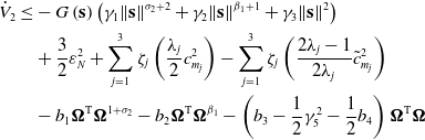 \begin{align} \dot{V}_{2}\leq &- G \left(\textbf{s}\right) \left(\gamma_{1}\|\textbf{s}\|^{\sigma_2+2}+ \gamma_{2}\|\textbf{s}\|^{\beta_1+1}+ \gamma_{3}\|\textbf{s}\|^{2}\right)\nonumber\\ & +\frac{3}{2}\varepsilon_{N}^{2} +\sum_{j=1}^{3}\zeta_{j}\left(\frac{\lambda_{j}}{2}c_{m_j}^{2}\right) -\sum_{j=1}^{3}\zeta_{j}\left(\frac{2\lambda_{j}-1}{2\lambda_{j}}\tilde{c}_{m_j}^{2} \right)\\ &-b_{1}\boldsymbol{\Omega}^{\text{T}}\boldsymbol{\Omega}^{1+\sigma_2} -b_{2}\boldsymbol{\Omega}^{\text{T}}\boldsymbol{\Omega}^{\beta_{1}} -\left( b_{3}-\frac{1}{2}\gamma_{5}^2-\frac{1}{2}b_{4}\right) \boldsymbol{\Omega}^{\text{T}}\boldsymbol{\Omega}\nonumber\end{align}
Choose parameters $ {b}_{3}$
,
$ {b}_{3}$
, $ {b}_{4}$
and
$ {b}_{4}$
and $ {\gamma }_{5}$
, such that
$ {\gamma }_{5}$
, such that $ {b}_{3}-\frac{1}{2}{\gamma }_{5}^{2}-\frac{1}{2}{b}_{4}\gt 0$
. Thus, one has
$ {b}_{3}-\frac{1}{2}{\gamma }_{5}^{2}-\frac{1}{2}{b}_{4}\gt 0$
. Thus, one has
 \begin{align} \dot{V}_{2}\leq & - \gamma_{1} G \left(\textbf{s}\right) 2^{\frac{\sigma_2+2}{2}} \left(\frac{1}{2} \textbf{s}^{\text{T}} \textbf{s}\right)^{\frac{\sigma_2+2}{2}} - \gamma_{2} G \left(\textbf{s}\right) 2^{\frac{\beta_1+1}{2}} \left(\frac{1}{2} \textbf{s}^{\text{T}} \textbf{s}\right)^{\frac{\beta_1+1}{2}}\nonumber \\ & -\sum_{j=1}^{3} \left(\frac{y_j}{2\eta_j} \tilde{c}_{m_j}^{2} \right)^{\frac{\sigma_2+2}{2}} -\sum_{j=1}^{3} \left(\frac{y_j}{2\eta_j} \tilde{c}_{m_j}^{2} \right)^{\frac{\beta_1+1}{2}} -2^{\frac{\sigma_2+2}{2}}b_{2}\left(\frac{1}{2}\boldsymbol{\Omega}^{\text{T}}\boldsymbol{\Omega}\right) ^{\frac{\sigma_2+2}{2}}\\ & -2^{\frac{\beta_1+1}{2}}b_{3}\left(\frac{1}{2}\boldsymbol{\Omega}^{\text{T}}\boldsymbol{\Omega}\right) ^{\frac{\beta_1+1}{2}}+\Delta\nonumber \end{align}
where $ {y}_{j}={\eta }_{j}{\zeta }_{j}\frac{2{\lambda }_{j}-1}{2{\lambda }_{j}}$
, and
$ {y}_{j}={\eta }_{j}{\zeta }_{j}\frac{2{\lambda }_{j}-1}{2{\lambda }_{j}}$
, and $ {\Delta }={\sum }_{j=1}^{3} {\left(\frac{{y}_{j}}{2{\eta }_{j}}{\tilde{c}}_{{m}_{j}}^{2}\right)}^{\frac{{\sigma }_{2}+2}{2}}+{\sum }_{j=1}^{3} {\left(\frac{{y}_{j}}{2{\eta }_{j}}{\tilde{c}}_{{m}_{j}}^{2}\right)}^{\frac{{\beta }_{1}+1}{2}}+{\sum }_{j=1}^{3} \left(\frac{{\zeta }_{j}{\lambda }_{j}}{2}{c}_{{m}_{j}}^{2}\right)-{\sum }_{j=1}^{3} \left(\frac{{y}_{j}}{{\eta }_{j}}{\tilde{c}}_{{m}_{j}}^{2}\right)+\frac{3}{2}{\epsilon }_{N}^{2}$
.
$ {\Delta }={\sum }_{j=1}^{3} {\left(\frac{{y}_{j}}{2{\eta }_{j}}{\tilde{c}}_{{m}_{j}}^{2}\right)}^{\frac{{\sigma }_{2}+2}{2}}+{\sum }_{j=1}^{3} {\left(\frac{{y}_{j}}{2{\eta }_{j}}{\tilde{c}}_{{m}_{j}}^{2}\right)}^{\frac{{\beta }_{1}+1}{2}}+{\sum }_{j=1}^{3} \left(\frac{{\zeta }_{j}{\lambda }_{j}}{2}{c}_{{m}_{j}}^{2}\right)-{\sum }_{j=1}^{3} \left(\frac{{y}_{j}}{{\eta }_{j}}{\tilde{c}}_{{m}_{j}}^{2}\right)+\frac{3}{2}{\epsilon }_{N}^{2}$
.
If $ \frac{{}_{j}}{2{\eta }_{j}}{\tilde{c}}_{{m}_{j}}^{2}\ge 1$
, the following inequality holds
$ \frac{{}_{j}}{2{\eta }_{j}}{\tilde{c}}_{{m}_{j}}^{2}\ge 1$
, the following inequality holds
 \begin{align} {\left(\frac{{y}_{j}}{2{\eta }_{j}}{\tilde{c}}_{{m}_{j}}^{2}\right)}^{\frac{{\sigma }_{2}+2}{2}}+{\left(\frac{{y}_{j}}{2{\eta }_{j}}{\tilde{c}}_{{m}_{j}}^{2}\right)}^{\frac{{\beta }_{1}+1}{2}}-\left(\frac{{y}_{j}}{{\eta }_{j}}{\tilde{c}}_{{m}_{j}}^{2}\right) & \le {\left(\frac{{y}_{j}}{2{\eta }_{j}}{\tilde{c}}_{{m}_{j}}^{2}\right)}^{\frac{{\sigma }_{2}+2}{2}}-\left(\frac{{y}_{j}}{2{\eta }_{j}}{\tilde{c}}_{{m}_{j}}^{2}\right)\nonumber\\[5pt]& \le {\left(\frac{{y}_{j}}{2{\eta }_{j}}{\tilde{c}}_{{m}_{j}}^{2}\right)}^{\frac{{\sigma }_{2}+2}{2}}-1\end{align}
On the other hand, for the case $ \frac{{y}_{j}}{2{\eta }_{j}}{\tilde{c}}_{{m}_{j}}^{2} \lt 1$
, it yields
$ \frac{{y}_{j}}{2{\eta }_{j}}{\tilde{c}}_{{m}_{j}}^{2} \lt 1$
, it yields
 \begin{align} {\left(\frac{{y}_{j}}{2{\eta }_{j}}{\tilde{c}}_{{m}_{j}}^{2}\right)}^{\frac{{\sigma }_{2}+2}{2}}+{\left(\frac{{y}_{j}}{2{\eta }_{j}}{\tilde{c}}_{{m}_{j}}^{2}\right)}^{\frac{{\beta }_{1}+1}{2}}-\left(\frac{{y}_{j}}{{\eta }_{j}}{\tilde{c}}_{{m}_{j}}^{2}\right)\le {\left(\frac{{y}_{j}}{2{\eta }_{j}}{\tilde{c}}_{{m}_{j}}^{2}\right)}^{\frac{{\beta }_{1}+1}{2}}-\left(\frac{{y}_{j}}{2{\eta }_{j}}{\tilde{c}}_{{m}_{j}}^{2}\right)\le 1\end{align}
According to the theory of uniform boundedness, $ \textbf{s}$
and
$ \textbf{s}$
and $ {\tilde{\textbf{c}}}_{m}$
are uniformly bounded. Therefore, there are always some positive constants
$ {\tilde{\textbf{c}}}_{m}$
are uniformly bounded. Therefore, there are always some positive constants $ {\vartheta }_{j}(j=\textrm{1,2},3)$
such that
$ {\vartheta }_{j}(j=\textrm{1,2},3)$
such that $ \left|{\tilde{c}}_{{m}_{j}}\right| \lt {\vartheta }_{j}$
. Then,
$ \left|{\tilde{c}}_{{m}_{j}}\right| \lt {\vartheta }_{j}$
. Then,
 \begin{align} {\Delta } & = \sum _{j=1}^{3} \left\{{\left(\frac{{y}_{j}}{2{\eta }_{j}}{\tilde{c}}_{{m}_{j}}^{2}\right)}^{\frac{{\sigma }_{2}+2}{2}}+{\left(\frac{{y}_{j}}{2{\eta }_{j}}{\tilde{c}}_{{m}_{j}}^{2}\right)}^{\frac{{\beta }_{1}+1}{2}}-\left(\frac{{y}_{j}}{{\eta }_{j}}{\tilde{c}}_{{m}_{j}}^{2}\right)\right\}\nonumber\\& +\sum _{j=1}^{3} \left(\frac{{\zeta }_{j}{\lambda }_{j}}{2}{c}_{{m}_{j}}^{2}\right)+\frac{3}{2}{\epsilon }_{N}^{2}\\ & \le \sum _{j=1}^{3} \textrm{m}\textrm{a}\textrm{x}\left\{{\left(\frac{{y}_{j}}{2{\eta }_{j}}{\vartheta }_{j}^{2}\right)}^{\frac{{\sigma }_{2}+2}{2}}-\textrm{1,1}\right\}+\sum _{j=1}^{3} \left(\frac{{\zeta }_{j}{\lambda }_{j}}{2}{c}_{{m}_{j}}^{2}\right)+\frac{3}{2}{\epsilon }_{N}^{2} \lt \infty \nonumber \end{align}
Using Lemma 1, the previous inequality Equation (43) is further simplified as
 \begin{align} \dot{{V}}_{2} \leq & - \gamma_{1} G \left(\textbf{s}\right) 2^{\frac{\sigma_2+2}{2}} \left(\frac{1}{2} \textbf{s}^{\text{T}} \textbf{s}\right)^{\frac{\sigma_2+2}{2}} -{y}_{m}\left(\frac{1}{2}{\tilde{\textbf{c}}}_{m}^{\text{T}}\boldsymbol{\eta}^{-1} {\tilde{\textbf{c}}}_{m} \right)^{\frac{\sigma_2+2}{2}}\nonumber\\ & -2^{\frac{\sigma_2+2}{2}}b_{2}\left(\frac{1}{2}\boldsymbol{\Omega}^{\text{T}}\boldsymbol{\Omega}\right) ^{\frac{\sigma_2+2}{2}} - \gamma_{2} G \left(\textbf{s}\right) 2^{\frac{\beta_1+1}{2}} \left(\frac{1}{2} \textbf{s}^{\text{T}} \textbf{s}\right)^{\frac{\beta_1+1}{2}} \\ & - {y}_{m}\left(\frac{1}{2} {\tilde{\textbf{c}}}_{m}^{\text{T}}\boldsymbol{\eta}^{-1} {\tilde{\textbf{c}}}_{m} \right)^{\frac{\beta_1+1}{2}} -2^{\frac{\beta_1+1}{2}}b_{3}\left(\frac{1}{2}\boldsymbol{\Omega}^{\text{T}}\boldsymbol{\Omega}\right) ^{\frac{\beta_1+1}{2}}+\Delta\nonumber\\ \leq & -a V_{2}^{\frac{\sigma_2+2}{2}} - b V_{2}^{\frac{\beta_1+1}{2}}+\Delta\nonumber \end{align}
where ${y_m} = {\rm{min}}\left\{ {y_1^{\frac{{{\sigma _2} + 2}}{2}},y_2^{\frac{{{\sigma _2} + 2}}{2}},y_3^{\frac{{{\sigma _2} + 2}}{2}}} \right\}$
,
${y_m} = {\rm{min}}\left\{ {y_1^{\frac{{{\sigma _2} + 2}}{2}},y_2^{\frac{{{\sigma _2} + 2}}{2}},y_3^{\frac{{{\sigma _2} + 2}}{2}}} \right\}$
, $a = {3^{ - \frac{{{\sigma _2}}}{2}}}{\rm{min}}\left\{ {{2^{\frac{{{\sigma _2} + 2}}{2}}}{\gamma _1}G\left( {\bf{s}} \right),{y_m},{2^{\frac{{{\sigma _2} + 2}}{2}}}{b_2}} \right\}$
,
$a = {3^{ - \frac{{{\sigma _2}}}{2}}}{\rm{min}}\left\{ {{2^{\frac{{{\sigma _2} + 2}}{2}}}{\gamma _1}G\left( {\bf{s}} \right),{y_m},{2^{\frac{{{\sigma _2} + 2}}{2}}}{b_2}} \right\}$
, $b = {\rm{min}}\{ {2^{\frac{{{\beta _1} + 1}}{2}}}{\gamma _2}G\left( {\bf{s}} \right),$ ${y_m},{2^{\frac{{{\beta _1} + 1}}{2}}}{b_3}\} $
.
${y_m},{2^{\frac{{{\beta _1} + 1}}{2}}}{b_3}\} $
.
Therefore, according to Lemma 3, it can be concluded that the NFTSS (13) is practically fixed-time stable and converges to the following residual set ${\rm{\Pi }}$
after a bounded time
${\rm{\Pi }}$
after a bounded time ${T_r}$
.
${T_r}$
.
 \begin{align}{\rm{\Pi }}: = \left\{ {\mathop {{\rm{lim}}}\limits_{t \to {T_r}} {\bf{s}}(t)|\parallel {\bf{s}}(t)\parallel \le {\rm{\Phi }}} \right\}\end{align}
where for $0 \lt {o_1},{o_2} \le 1$
,
$0 \lt {o_1},{o_2} \le 1$
,
 \begin{align}{\rm{\Phi }} = {\rm{min}}\left\{ {{{\left( {\frac{{\rm{\Delta }}}{{a\left( {1 - {o_1}} \right)}}} \right)}^{\frac{2}{{{\sigma _2} + 2}}}},{{\left( {\frac{{\rm{\Delta }}}{{b\left( {1 - {o_2}} \right)}}} \right)}^{\frac{2}{{{\beta _1} + 1}}}}} \right\}\end{align}
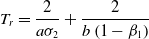 \begin{align}{T_r} = \frac{2}{{a{\sigma _2}}} + \frac{2}{{b\left( {1 - {\beta _1}} \right)}}\end{align}
-
Step 2. Once
$s$
reaches the region
$\Pi $
, the fixed-time convergence property of the system states should be demonstrated by the following analysis.


Case 1. If ${\bf{s}} = 0$
is reached, then
${\bf{s}} = 0$
is reached, then $\overline {{s_i}} = 0$
. Based on Lemma 4, the fixed-time convergence of tracking error
$\overline {{s_i}} = 0$
. Based on Lemma 4, the fixed-time convergence of tracking error ${{\bf{e}}_1}$
and velocity error
${{\bf{e}}_1}$
and velocity error ${{\bf{e}}_2}$
can be guaranteed during the sliding phase.
${{\bf{e}}_2}$
can be guaranteed during the sliding phase.
Case 2. In the case of $\overline {{s_i}} \ne 0$
and
$\overline {{s_i}} \ne 0$
and $\left| {{e_{1i}}} \right| \ge $ ${\varepsilon _0}$
, let
${\varepsilon _0}$
, let ${s_i} = {\phi _i} \in {\rm{\Pi }}$
and one has
${s_i} = {\phi _i} \in {\rm{\Pi }}$
and one has
 \begin{align}s_{i}=e_{2i}+ N\left(\textbf{e}_1\right) \left( K_{1i}\textrm{sig}^{1+\sigma_{1}}(e_{1i}) +K_{2i}\textrm{sig}^{\frac{p}{q}}(e_{1i}) \right) =\phi_{i}\end{align}
it follows that
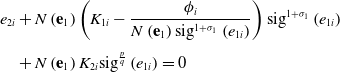 \begin{align}{{e_{2i}}} & + N\left( {{{\bf{e}}_1}} \right)\left( {{K_{1i}} - \frac{{{\phi _i}}}{{N\left( {{{\bf{e}}_1}} \right){\rm{si}}{{\rm{g}}^{1 + {\sigma _1}}}\left( {{e_{1i}}} \right)}}} \right){\rm{si}}{{\rm{g}}^{1 + {\sigma _1}}}\left( {{e_{1i}}} \right)\nonumber\\[4pt]& + N\left( {{{\bf{e}}_1}} \right){K_{2i}}{\rm{si}}{{\rm{g}}^{\frac{p}{q}}}\left( {{e_{1i}}} \right) = 0\end{align}
 \begin{align}{{e_{2i}}} & + N\left( {{{\bf{e}}_1}} \right){K_{1i}}{\rm{si}}{{\rm{g}}^{1 + {\sigma _1}}}\left( {{e_{1i}}} \right)\nonumber\\[4pt]& + N\left( {{{\bf{e}}_1}} \right)\left( {{K_{2i}} - \frac{{{\phi _i}}}{{N\left( {{{\bf{e}}_1}} \right){\rm{si}}{{\rm{g}}^{\frac{p}{q}}}\left( {{e_{1i}}} \right)}}} \right){\rm{si}}{{\rm{g}}^{\frac{p}{q}}}\left( {{e_{1i}}} \right) = 0\end{align}
Choosing ${K_{1i}}$
such that
${K_{1i}}$
such that ${K_{1i}} - \dfrac{{{\phi _i}}}{{N\left( {{{\bf{e}}_1}} \right){\rm{si}}{{\rm{g}}^{1 + {\sigma _1}}}\left( {{e_{1i}}} \right)}} \gt 0$
or
${K_{1i}} - \dfrac{{{\phi _i}}}{{N\left( {{{\bf{e}}_1}} \right){\rm{si}}{{\rm{g}}^{1 + {\sigma _1}}}\left( {{e_{1i}}} \right)}} \gt 0$
or ${K_{2i}} - \dfrac{{{\phi _i}}}{{N\left( {{{\bf{e}}_1}} \right){\rm{si}}{{\rm{g}}^{\dfrac{p}{q}}}\left( {{e_{1i}}} \right)}} \gt 0$
, then the fixed-time stability of the system can still be guaranteed. Therefore, the tracking error
${K_{2i}} - \dfrac{{{\phi _i}}}{{N\left( {{{\bf{e}}_1}} \right){\rm{si}}{{\rm{g}}^{\dfrac{p}{q}}}\left( {{e_{1i}}} \right)}} \gt 0$
, then the fixed-time stability of the system can still be guaranteed. Therefore, the tracking error ${e_{1i}}$
ultimately converges to the region
${e_{1i}}$
ultimately converges to the region $\left| {{e_{1i}}} \right| \le {{\rm{\Psi }}_{e1}}$
after a fixed time. At this time, it is easy to derive that the tracking velocity
$\left| {{e_{1i}}} \right| \le {{\rm{\Psi }}_{e1}}$
after a fixed time. At this time, it is easy to derive that the tracking velocity ${e_{2i}}$
converges to the region
${e_{2i}}$
converges to the region $\left| {{e_{2i}}} \right| \le {{\rm{\Psi }}_{e2}}$
after a fixed time.
$\left| {{e_{2i}}} \right| \le {{\rm{\Psi }}_{e2}}$
after a fixed time.
Case 3. For the case ${\bar s_i} \ne 0$
and
${\bar s_i} \ne 0$
and $\left| {{e_{1i}}} \right| \lt $ ${\varepsilon _0}$
. Since the tracking error
${\varepsilon _0}$
. Since the tracking error ${e_{1i}}$
has entered the region
${e_{1i}}$
has entered the region ${{\rm{\Psi }}_{e1}}$
, according to the NFTSS (13), one obtains
${{\rm{\Psi }}_{e1}}$
, according to the NFTSS (13), one obtains
 \begin{align}{s_i} = {e_{2i}} + N\left( {{{\bf{e}}_1}} \right)\left( {{K_{1i}}{\rm{si}}{{\rm{g}}^{1 + {\sigma _1}}}\left( {{e_{1i}}} \right) + {K_{2i}}\left( {{l_1}{e_{1i}} + {l_2}e_{1i}^2{\rm{sgn}}\left( {{e_{1i}}} \right)} \right)} \right) = {\phi _i}\end{align}
It follows that
 \begin{align}\left| {{e_{2i}}} \right| \le {\phi _i} + N\left( {{{\bf{e}}_1}} \right)\left( {{K_{1i}}\left| {{e_1}{|^{1 + {\sigma _1}}} + {K_{2i}}} \right|{l_1}{e_{1i}} + {l_2}e_{1i}^2{\rm{sgn}}\left( {{e_{1i}}} \right)|} \right) \le {{\rm{\Psi }}_{{e_2}}}\end{align}
The above analysis shows that the system states ${e_{1i}}$
and
${e_{1i}}$
and ${e_{2i}}$
will converge to the sets
${e_{2i}}$
will converge to the sets $\left| {{e_{1i}}} \right| \le {{\rm{\Psi }}_{e1}}$
and
$\left| {{e_{1i}}} \right| \le {{\rm{\Psi }}_{e1}}$
and $\left| {{e_{2i}}} \right| \le {{\rm{\Psi }}_{e2}}$
after a fixed time, respectively. It is concluded that the closed-loop tracking control system is practically fixed-time stable. The proof is completed.
$\left| {{e_{2i}}} \right| \le {{\rm{\Psi }}_{e2}}$
after a fixed time, respectively. It is concluded that the closed-loop tracking control system is practically fixed-time stable. The proof is completed.
Remark 7. Appropriate control parameters are crucial for achieving improved control accuracy when adopting the suggested control scheme into practice. Therefore, here are some suggestions for parameter selection:
-
(a) According to Equation (14), the selection of
${\varepsilon _0}$
will have a direct impact on the effectiveness of the singularity problem solution, directly affecting the convergence accuracy of the system state. -
(b) Larger
${K_{1i}}$
and
${K_{2i}}$
will result in a faster convergence rate at the cost of more control energy consumption in the initial response, especially when the initial state is far from the equilibrium point. -
(c) For the purpose of tracking control with high precision,
${\varepsilon _N}$
should be selected small enough, which leads to a greater control input. Therefore, a trade-off between the control effort and the system performance is required. -
(d) Unexpected changes in the control inputs may have a negative effect on the actuator. The influence of the actuator saturation on the auxiliary system can be mitigated by adjusting the value of the parameter
${b_4}$
, particularly in cases when the actuator saturation is significant. -
(e) The settling time expression Equation (21) indicates that the parameters
$q$
,
$p$
,
${n_1}$
and
${m_1}$
are also crucial in dominating the convergence rate and accuracy.Figure 4. D-H model of the studied space manipulator system.


4.0 Numerical simulations
In this section, numerical simulations of a seven-degrees-of-freedom free-floating space manipulator system are conducted in two parts to evaluate the performance of the proposed adaptive fixed-time control strategy. The D-H model and physical parameters of the studied system are shown in Fig. 4 and Table 1, respectively. In this simulation, considering the system uncertainties, the nominal mass values of the system are set as ${m_{B0}} = 90\,{\rm{kg}}$
,
${m_{B0}} = 90\,{\rm{kg}}$
, ${m_{B1}} = 3.825{\rm{kg}}$
,
${m_{B1}} = 3.825{\rm{kg}}$
, ${m_{B2}} = 6.3{\rm{kg}}$
,
${m_{B2}} = 6.3{\rm{kg}}$
, ${m_{B3}} = 6.3{\rm{kg}}$
,
${m_{B3}} = 6.3{\rm{kg}}$
, ${m_{B4}} = 3.825{\rm{kg}}$
,
${m_{B4}} = 3.825{\rm{kg}}$
, ${m_{B5}} = 3.825{\rm{kg}}$
,
${m_{B5}} = 3.825{\rm{kg}}$
, ${m_{B6}} = 3.825{\rm{kg}}$
and
${m_{B6}} = 3.825{\rm{kg}}$
and ${m_{B7}} = 3.825{\rm{kg}}$
. And the time-varying disturbances acted on the system are given by
${m_{B7}} = 3.825{\rm{kg}}$
. And the time-varying disturbances acted on the system are given by ${\bf{d}}(t) = [0.03{\rm{sin}}(t) + 0.005sin\left( {200\pi t} \right), 0.03{\rm{sin}}\left( {2t} \right) + 0.005{\rm{sin}}\left( {200\pi t} \right),0.01{\rm{sin}}(t) +$ $ 0.002{\rm{sin}}\left( {200\pi t} \right),\,\,0.01{\rm{sin}}\left( {2t} \right) \,+\, 0.001{\rm{sin}}\left( {200\pi t} \right),\,\,0.02{\rm{sin}}(t) \,+\, 0.002{\rm{sin}}\left( {200\pi t} \right),\,\,0.01{\rm{sin}}\left( {3t} \right) + $ $0.001{\rm{sin}}\left( {200\pi t} \right),0.02{\rm{sin}}\left( {3t} \right) + 0.003{\rm{sin}}\left( {200\pi t} \right)]^{\rm{T}}{\rm{N}} \cdot {\rm{m}}.$
The initial state of the spacecraft base is chosen as
$0.001{\rm{sin}}\left( {200\pi t} \right),0.02{\rm{sin}}\left( {3t} \right) + 0.003{\rm{sin}}\left( {200\pi t} \right)]^{\rm{T}}{\rm{N}} \cdot {\rm{m}}.$
The initial state of the spacecraft base is chosen as ${[0,0,0,1,0,0,0]^{\rm{T}}}$
. The joint initial and desired configurations are assigned as
${[0,0,0,1,0,0,0]^{\rm{T}}}$
. The joint initial and desired configurations are assigned as ${[0,\pi /3,0,\pi /4,\pi /4,0,\pi /6]^{\rm{T}}}$
rad and
${[0,\pi /3,0,\pi /4,\pi /4,0,\pi /6]^{\rm{T}}}$
rad and $[0.15 - 0.14{{\rm{e}}^{ - t}} + 0.07{e^{ - 2t}},1.05 + 0.1{{\rm{e}}^ - } - 0.05{e^{ - 2t}}, s0.17 + 0.1{{\rm{e}}^{ - 2t}} - 0.2{e^{ - t}},0.48 - 0.1{{\rm{e}}^{ - 3t}} + 0.3{e^{ - t}},0.8 - 0.05{{\rm{e}}^{ - 2t}} {+} 0.1{e^{ - t}}, - 0.2 + 0.2{{\rm{e}}^{ - t}} - 0.1{e^{ - 2t}},0.7 + 0.25{{\rm{e}}^{ - 2t}} - 0.5{e^{ - t}}]^{\rm{T}}$
rad. The parameters of the prescribed performance boundary are set as
$[0.15 - 0.14{{\rm{e}}^{ - t}} + 0.07{e^{ - 2t}},1.05 + 0.1{{\rm{e}}^ - } - 0.05{e^{ - 2t}}, s0.17 + 0.1{{\rm{e}}^{ - 2t}} - 0.2{e^{ - t}},0.48 - 0.1{{\rm{e}}^{ - 3t}} + 0.3{e^{ - t}},0.8 - 0.05{{\rm{e}}^{ - 2t}} {+} 0.1{e^{ - t}}, - 0.2 + 0.2{{\rm{e}}^{ - t}} - 0.1{e^{ - 2t}},0.7 + 0.25{{\rm{e}}^{ - 2t}} - 0.5{e^{ - t}}]^{\rm{T}}$
rad. The parameters of the prescribed performance boundary are set as ${\rho _0} = 0.15$
,
${\rho _0} = 0.15$
, ${\rho _\infty } = 5 \times {10^{ - 6}}$
, and
${\rho _\infty } = 5 \times {10^{ - 6}}$
, and ${l_0} = 2.5$
. The controller parameters are listed in Table 2.
${l_0} = 2.5$
. The controller parameters are listed in Table 2.
Table 1. Physical parameters of the studied space manipulator
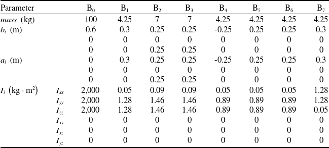
Table 2. Parameters of the proposed controller
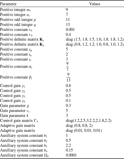
4.1 Performance evaluation with healthy actuators
In this part, the input saturation is ignored, and the main purpose is to investigate the effect of the PPC constraint on the tracking performance. The proposed control scheme is compared with an adaptive fixed-time sliding mode controller (AFSMTC) that does not take into account performance constraints. The AFSMTC has the same form as the proposed scheme, except for the tan-type PPC term. For a fair comparison, the control parameters chosen for the AFSMTC are identical to those of the proposed scheme. The simulation results are given in Figs 5–8.
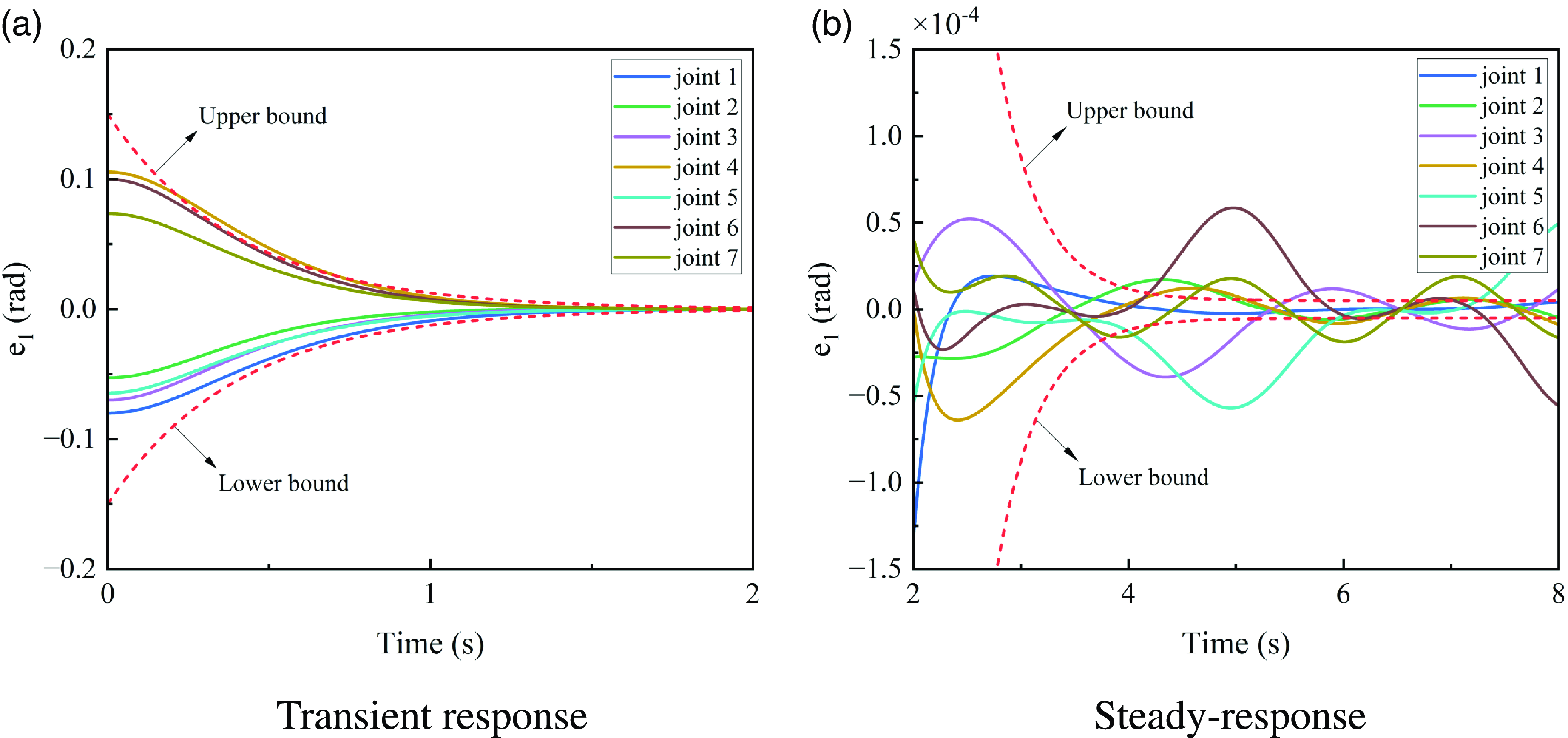
Figure 5. Time response of position tracking error under the AFSMTC.
Figure 6. Time response of position tracking error under the proposed controller.
Figure 7. Time response of velocity tracking error.
Figure 8. Time response of control torques.
Figures 5–7 illustrate the time responses of the position and velocity tracking errors. These results validate the stability analysis in Section 3 comfortably. Although both controllers enable fixed-time convergence, the proposed controller possesses a faster transient response with higher steady-state accuracy. Furthermore, with the help of tan-type PPC, the position tracking errors are always strictly limited to the predefined boundary in both transient and steady-state phases, whereas those of the AFSMTC violate the constraint. As can be seen, since the constraint boundary is decaying with time, the norm of tracking error is decreasing, which increases the tracking precision. It is the effect of the prescribed performance function in the proposed control scheme. Control torques are depicted in Fig. 8, from which the maximum torque required by the proposed controller is slightly larger than that of the AFSMTC. This is because the control gain is increased to counteract the evolution of the tracking error when it approaches the constraint boundary. It is worth noting that to obtain fast trajectory tracking, both controllers have a large transient response at the beginning of the movement, which can make them impossible for practical applications. Therefore, the influence of actuator saturation needs to be considered during the controller design process.
4.2 Performance evaluation with input saturation
In this part, the problem of input saturation is investigated and the capability of the proposed controller is evaluated in the following two simulation sections. To this end, the allowable maximum input control torques are selected as ${[60,50,35,25,25,20,30]^{\rm{T}}}{\rm{N}} \cdot {\rm{m}}$
.
${[60,50,35,25,25,20,30]^{\rm{T}}}{\rm{N}} \cdot {\rm{m}}$
.
4.2.1 Performance validation of the saturation compensator
In this simulation, the main objective is to illustrate the effectiveness of the proposed saturation compensator in the proposed control method, two cases are discussed for comparison. One is the tracking control with saturation compensation, and the other is the tracking control without saturation compensation.
The simulation results without and with saturation compensation are presented in Figs 9 and 10, respectively. As shown in Fig. 9, the convergence time of tracking error and tracking speed error is finite, but the error constraint boundary is no longer satisfied. It indicates that input saturation has greatly attenuated the convergence performance of trajectory tracking. From Fig. 10, the predicted compensation parameter ${\bf{\Omega }}$
converges quickly to a constant, which means a strong compensation role when starting to track the desired trajectory. Under the action of the saturation compensator, the tracking error is not only always strictly remained within the predefined constraint bounds, but also a superior control performance is obtained with shorter settling time and faster convergence speed. By comparison, the actual control torques for both controllers are guaranteed to be within their maximum allowable limits. It should be noted that due to the influence of input saturation, the torque produces a strong chattering phenomenon. Whereas with the help of the saturation compensator, the control torque obtained is smoother with significantly less chattering. To sum up, conclusions can be drawn the proposed saturation compensator can eliminate the effect of input saturation to a certain extent and accelerate the convergence rate of trajectory tracking in the proposed control scheme.
${\bf{\Omega }}$
converges quickly to a constant, which means a strong compensation role when starting to track the desired trajectory. Under the action of the saturation compensator, the tracking error is not only always strictly remained within the predefined constraint bounds, but also a superior control performance is obtained with shorter settling time and faster convergence speed. By comparison, the actual control torques for both controllers are guaranteed to be within their maximum allowable limits. It should be noted that due to the influence of input saturation, the torque produces a strong chattering phenomenon. Whereas with the help of the saturation compensator, the control torque obtained is smoother with significantly less chattering. To sum up, conclusions can be drawn the proposed saturation compensator can eliminate the effect of input saturation to a certain extent and accelerate the convergence rate of trajectory tracking in the proposed control scheme.
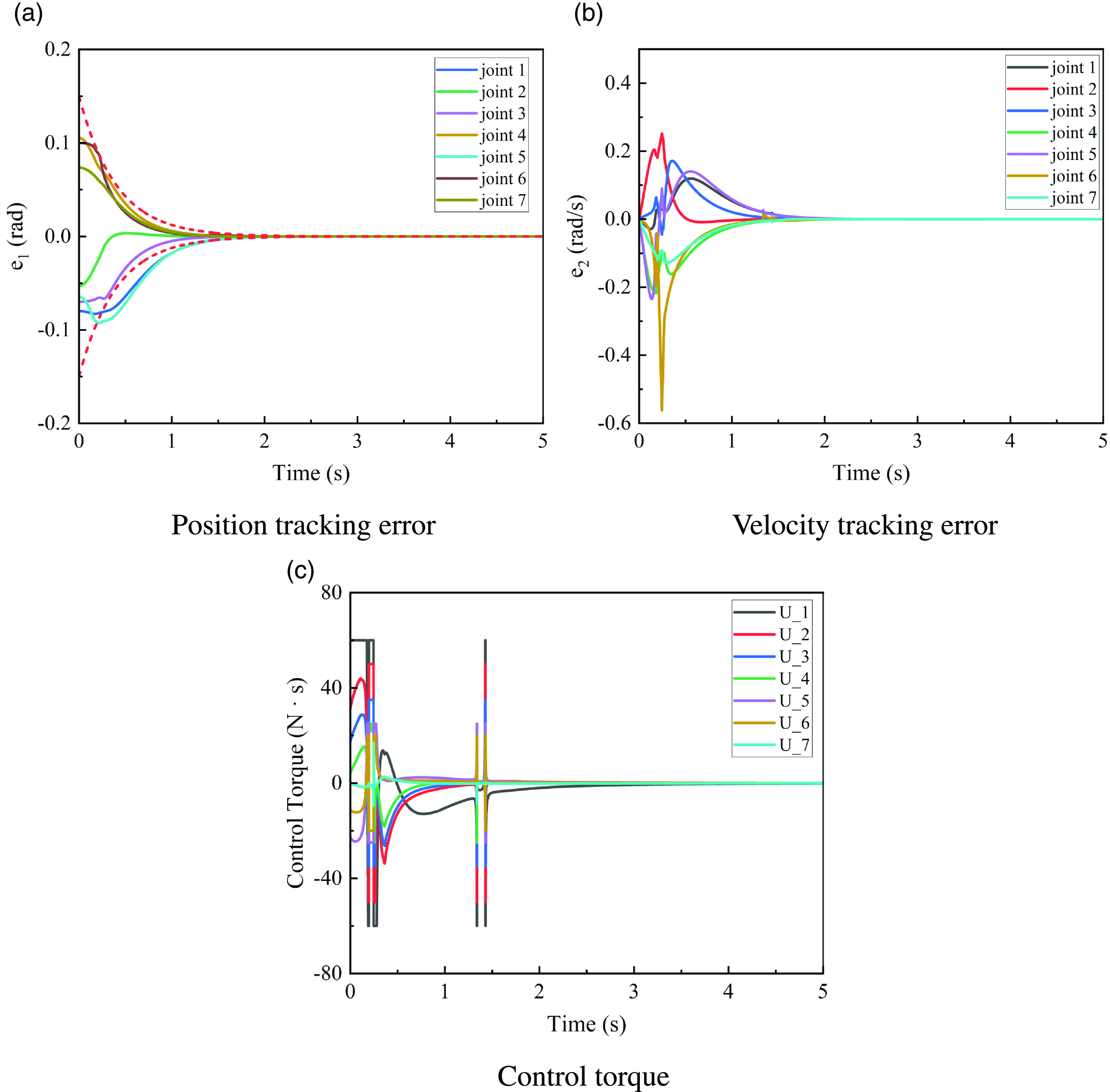
Figure 9. Simulation results without the saturation compensator.

Figure 10. Simulation results with the saturation compensator.
4.2.2 Performance comparison with existing mehtods
To further assess the proposed controller’s performance, comparisons are performed with the existing fixed-time control strategies proposed in Refs [Reference Zuo18, Reference Zhang, Tang and Guo47]. To ensure the rationality of the comparison, all simulation experiments are conducted under the same initial conditions. The FTSMC can be described as follows [Reference Zuo18]:
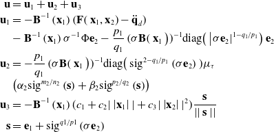 \begin{align} \textbf{u} & ={\textbf{u}}_{1}+{\textbf{u}}_{2}+{\textbf{u}}_{3}\nonumber\\[-2pt] {\textbf{u}}_{1} & =-{\textbf{B}}^{-1}\left({\textbf{x}}_{1}\right)\left(\textbf{F}\right({\textbf{x}}_{1},{\textbf{x}}_{2})-{\ddot{\textbf{q}}}_{d})\nonumber\\[-2pt] & -{\textbf{B}}^{-1}\left({\textbf{x}}_{1}\right){\sigma }^{-1}{\Phi }{\textbf{e}}_{2}-\frac{{p}_{1}}{{q}_{1}}\left(\sigma \textbf{B}\right({\textbf{x}}_{1}\left){)}^{-1}\textrm{d}\textrm{i}\textrm{a}\textrm{g}\right(\left|\sigma {\textbf{e}}_{2}{|}^{1-{q}_{1}/{p}_{1}}\right){\textbf{e}}_{2}\nonumber\\[-2pt] {\textbf{u}}_{2} & =-\frac{{p}_{1}}{{q}_{1}}\left(\sigma \textbf{B}\right({\textbf{x}}_{1}\left){)}^{-1}\textrm{d}\textrm{i}\textrm{a}\textrm{g}\right(\textrm{s}\textrm{i}{\textrm{g}}^{2-{q}_{1}/{p}_{1}}\left(\sigma {\textbf{e}}_{2}\right)){\mu }_{\tau }\nonumber\\[-2pt] & \left({\alpha }_{2}\textrm{s}\textrm{i}{\textrm{g}}^{{m}_{2}/{n}_{2}}\left(\textbf{s}\right)+{\beta }_{2}\textrm{s}\textrm{i}{\textrm{g}}^{{p}_{2}/{q}_{2}}\left(\textbf{s}\right)\right)\\[-2pt] {\textbf{u}}_{3} & =-{\textbf{B}}^{-1}\left({\textbf{x}}_{1}\right)({c}_{1}+{c}_{2}|\left|{\textbf{x}}_{1}\right||+{c}_{3}|\left|{\textbf{x}}_{2}\right|{|}^{2})\frac{\textbf{s}}{\left|\right|\textbf{s}\left|\right|}\nonumber\\[-2pt] \textbf{s} & ={\textbf{e}}_{1}+\textrm{s}\textrm{i}{\textrm{g}}^{q1/p1}\left(\sigma {\textbf{e}}_{2}\right)\nonumber \end{align}
where ${\alpha _2} \gt 0,{\beta _2} \gt 0$
,
${\alpha _2} \gt 0,{\beta _2} \gt 0$
, ${c_1},{c_2},{c_3}$
are three positive constants,
${c_1},{c_2},{c_3}$
are three positive constants, $\sigma = {\rm{diag}}\left( {{\sigma _1},{\sigma _2}, \ldots ,{\sigma _n}} \right)$
with
$\sigma = {\rm{diag}}\left( {{\sigma _1},{\sigma _2}, \ldots ,{\sigma _n}} \right)$
with ${\sigma _i} = \frac{1}{{{\alpha _1}\left( i \right)e_{1i}^{{m_1}/{n_1} - {p_1}/{q_1}} + {\beta _1}\left( i \right)}}$
,
${\sigma _i} = \frac{1}{{{\alpha _1}\left( i \right)e_{1i}^{{m_1}/{n_1} - {p_1}/{q_1}} + {\beta _1}\left( i \right)}}$
, ${\alpha _1} = \left[ {{\alpha _{11}},{\alpha _{12}}, \ldots ,{\alpha _{1n}}} \right]$
and
${\alpha _1} = \left[ {{\alpha _{11}},{\alpha _{12}}, \ldots ,{\alpha _{1n}}} \right]$
and ${\beta _1} = \left[ {{\beta _{11}},{\beta _{12}}, \ldots ,{\beta _{1n}}} \right]$
with
${\beta _1} = \left[ {{\beta _{11}},{\beta _{12}}, \ldots ,{\beta _{1n}}} \right]$
with ${\alpha _{1i}} \gt 0$
and
${\alpha _{1i}} \gt 0$
and ${\beta _{1i}} \gt 0$
,
${\beta _{1i}} \gt 0$
, ${\bf{\Phi }} = {\rm{diag}}\left( {{{\rm{\Phi }}_1},{{\rm{\Phi }}_2}, \ldots ,{{\rm{\Phi }}_n}} \right)$
with
${\bf{\Phi }} = {\rm{diag}}\left( {{{\rm{\Phi }}_1},{{\rm{\Phi }}_2}, \ldots ,{{\rm{\Phi }}_n}} \right)$
with ${{\rm{\Phi }}_i} = - {\alpha _{1i}}\left( {\frac{{{m_1}}}{{{n_1}}} - \frac{{{p_1}}}{{{q_1}}}} \right)e_{1i}^{{m_1}/{n_1} - {p_1}/{q_1} - 1}\sigma _i^2{e_{2i}}$
,
${{\rm{\Phi }}_i} = - {\alpha _{1i}}\left( {\frac{{{m_1}}}{{{n_1}}} - \frac{{{p_1}}}{{{q_1}}}} \right)e_{1i}^{{m_1}/{n_1} - {p_1}/{q_1} - 1}\sigma _i^2{e_{2i}}$
, ${m_1}$
,
${m_1}$
, ${m_2}$
,
${m_2}$
, ${n_1}$
,
${n_1}$
, ${n_2}$
,
${n_2}$
, ${p_1}$
,
${p_1}$
, ${p_2}$
,
${p_2}$
, ${q_1}$
,
${q_1}$
, ${q_2}$
are positive odd integers satisfying
${q_2}$
are positive odd integers satisfying ${m_1} \gt {n_1},{m_2} \gt {n_2},{p_1} \lt {q_1} \lt 2{p_1},{p_2} \lt {q_2}$
and
${m_1} \gt {n_1},{m_2} \gt {n_2},{p_1} \lt {q_1} \lt 2{p_1},{p_2} \lt {q_2}$
and ${m_1}/{n_1} - {p_1}/{q_1} \gt 1$
.
${m_1}/{n_1} - {p_1}/{q_1} \gt 1$
. ${\mu _\tau } = {\rm{diag}}\left( {{\mu _{\tau 1}},{\mu _{\tau 2}}, \ldots ,{\mu _{\tau n}}} \right)$
with
${\mu _\tau } = {\rm{diag}}\left( {{\mu _{\tau 1}},{\mu _{\tau 2}}, \ldots ,{\mu _{\tau n}}} \right)$
with ${\mu _{\tau i}}$
given by:
${\mu _{\tau i}}$
given by:
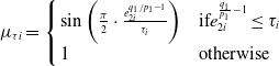 \begin{align}{\mu _{\tau i}} = \left\{ {\begin{array}{l@{\quad}l}{{\rm{sin}}\left( {\frac{\pi }{2} \cdot \frac{{e_{2i}^{{q_1}/{p_1} - 1}}}{{{\tau _i}}}} \right)} & {{\rm{if}}e_{2i}^{\frac{{{q_1}}}{{{p_1}}} - 1} \le {\tau _i}}\\1 & {{\rm{otherwise}}}\end{array}} \right.\end{align}
The value of ${\mu _{\tau i}}$
is 1 as the initial tracking speed
${\mu _{\tau i}}$
is 1 as the initial tracking speed ${{\bf{e}}_2}\left( 0 \right) = 0$
.
${{\bf{e}}_2}\left( 0 \right) = 0$
.
The adaptive nonsingular fast terminal sliding mode control (ANFTSMC) scheme proposed by Ref. [Reference Zhang, Tang and Guo47] is written as
 \begin{align}\textbf{u}&=\textbf{u}_1+\textbf{u}_{2}+\textbf{u}_{3}\nonumber\\ \textbf{u}_{1}&=-\textbf{B}^{-1}\left(\textbf{x}_{1}\right) \left(\textbf{F}\left(\textbf{x}_{1},\textbf{x}_{2}\right) -\ddot{\textbf{q}}_{d} \right)\nonumber\\ &\quad -\textbf{B}^{-1}\left(\textbf{x}_{1}\right) \left( k_1 \textbf{K}_{a} \textrm{diag}(\mid e_{1i}\mid^{k_1-1}) \textbf{e}_{2} +\textbf{K}_{b} \dot{\textbf{s}}_\rho(\textbf{e}_{1}) \right)\nonumber\\ \textbf{u}_{2}&= -\textbf{B}^{-1}\left(\textbf{x}_{1}\right) \left( \alpha_{2} {\textrm{sig}}^{k_2}(\textbf{s}) + \beta_{2} {\textrm{sig}}^{p_2/q_2}(\textbf{s}) \right)\nonumber\\ \textbf{u}_{3}&=-\textbf{B}^{-1}\left(\textbf{x}_{1}\right) \left(\hat{c}_{1}+\hat{c}_{2}\|{\boldsymbol{\boldsymbol{x}}_{1}}\|+\hat{c}_{3}\|\boldsymbol{\textbf{x}}_{2}\|^{2}\right) \tanh (\boldsymbol{s} / \varepsilon)\\\dot{\hat{c}}_{1}&=\eta_{11}\left(\boldsymbol{s}^{T} \tanh (\boldsymbol{s} / \varepsilon)-\eta_{21} \hat{c}_{1}\right)\nonumber\\ \dot{\hat{c}}_{2}&=\eta_{12}\left(\|{\boldsymbol{x}_1}\| \boldsymbol{s}^{T} \tanh (\boldsymbol{s} / \varepsilon)-\eta_{22} \hat{c}_{2}\right)\nonumber\\\dot{\hat{c}}_{3}&=\eta_{13}\left(\|\boldsymbol{x}_{2}\|^{2} \boldsymbol{s}^{T} \tanh (\boldsymbol{s} / \varepsilon)-\eta_{23} \hat{b}_{3}\right)\nonumber\\\textbf{s}&=\textbf{e}_{2}+\textbf{K}_{a}\textrm{sig}^{k_1 }(\textbf{e}_{1})+ \textbf{K}_{b}\textbf{s}_{\rho}(\textbf{e}_{1})\nonumber\end{align}
where ${{\bf{K}}_a},{{\bf{K}}_b}$
are positive definite matrices,
${{\bf{K}}_a},{{\bf{K}}_b}$
are positive definite matrices, ${\alpha _2} \gt 0,{\beta _2} \gt 0,$ ${k_1} = \frac{1}{2} + \frac{{{m_1}}}{{2{n_1}}} + \left( {\frac{{{m_1}}}{{2{n_1}}} - \frac{1}{2}} \right){\rm{sign}}\left( {\left| {\left| {{{\bf{e}}_1} - 1} \right|} \right|} \right)$
,
${k_1} = \frac{1}{2} + \frac{{{m_1}}}{{2{n_1}}} + \left( {\frac{{{m_1}}}{{2{n_1}}} - \frac{1}{2}} \right){\rm{sign}}\left( {\left| {\left| {{{\bf{e}}_1} - 1} \right|} \right|} \right)$
, ${k_2} = \frac{1}{2} + \frac{{{m_2}}}{{2{n_2}}} + \left( {\frac{{{m_2}}}{{2{n_2}}} - \frac{1}{2}} \right){\rm{sign}}\left( {\left| {\left| {{\bf{s}} - 1} \right|} \right|} \right)$
,
${k_2} = \frac{1}{2} + \frac{{{m_2}}}{{2{n_2}}} + \left( {\frac{{{m_2}}}{{2{n_2}}} - \frac{1}{2}} \right){\rm{sign}}\left( {\left| {\left| {{\bf{s}} - 1} \right|} \right|} \right)$
, ${m_1},{m_2},{p_1}$
and
${m_1},{m_2},{p_1}$
and ${p_2}$
are positive odd integers satisfying
${p_2}$
are positive odd integers satisfying ${m_1} \gt {n_1},{m_2} \gt {n_2}$
and
${m_1} \gt {n_1},{m_2} \gt {n_2}$
and ${p_2} \lt {q_2}$
,
${p_2} \lt {q_2}$
, ${\rm{tanh}}\left( {\frac{{\bf{s}}}{\varepsilon }} \right) = {[{\rm{tanh}}\left( {\frac{{{s_1}}}{\varepsilon }} \right),{\rm{tanh}}\left( {\frac{{{s_2}}}{\varepsilon }} \right), \ldots ,{\rm{tanh}}\left( {\frac{{{s_n}}}{\varepsilon }} \right)]^T}$
with
${\rm{tanh}}\left( {\frac{{\bf{s}}}{\varepsilon }} \right) = {[{\rm{tanh}}\left( {\frac{{{s_1}}}{\varepsilon }} \right),{\rm{tanh}}\left( {\frac{{{s_2}}}{\varepsilon }} \right), \ldots ,{\rm{tanh}}\left( {\frac{{{s_n}}}{\varepsilon }} \right)]^T}$
with $\varepsilon $
is a arbitrary small positive constant,
$\varepsilon $
is a arbitrary small positive constant, ${\eta _{1j}}$
and
${\eta _{1j}}$
and ${\eta _{2j}}$
are positive constants.
${\eta _{2j}}$
are positive constants.
Table 3. Controller parameters for FTSMC and ANFTSMC
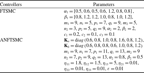
Generally, the faster the system responses, the larger control torques generates, resulting in more energy consumption. Therefore, the selection of control parameters requires a trade-off between control performances and input torques. The control parameters for FTSMC and ANFTSMC are listed in Table 3. Figures 11–12 give the response curves of the position and speed tracking errors under these different controllers. The convergence time of all controllers is observed to be bounded, and the suggested controller takes less time to track the desired trajectory than the other two controllers. Meanwhile, the transient performance requirement is consistently guaranteed only under the proposed control, implying that a quicker convergence performance is realised. Figure 13 clearly depicts the comparison of joint torques. In the presence of input saturation, the proposed controller provides a smoother, more continuous and less chattering control input.

Figure 11. Position tracking error performance.
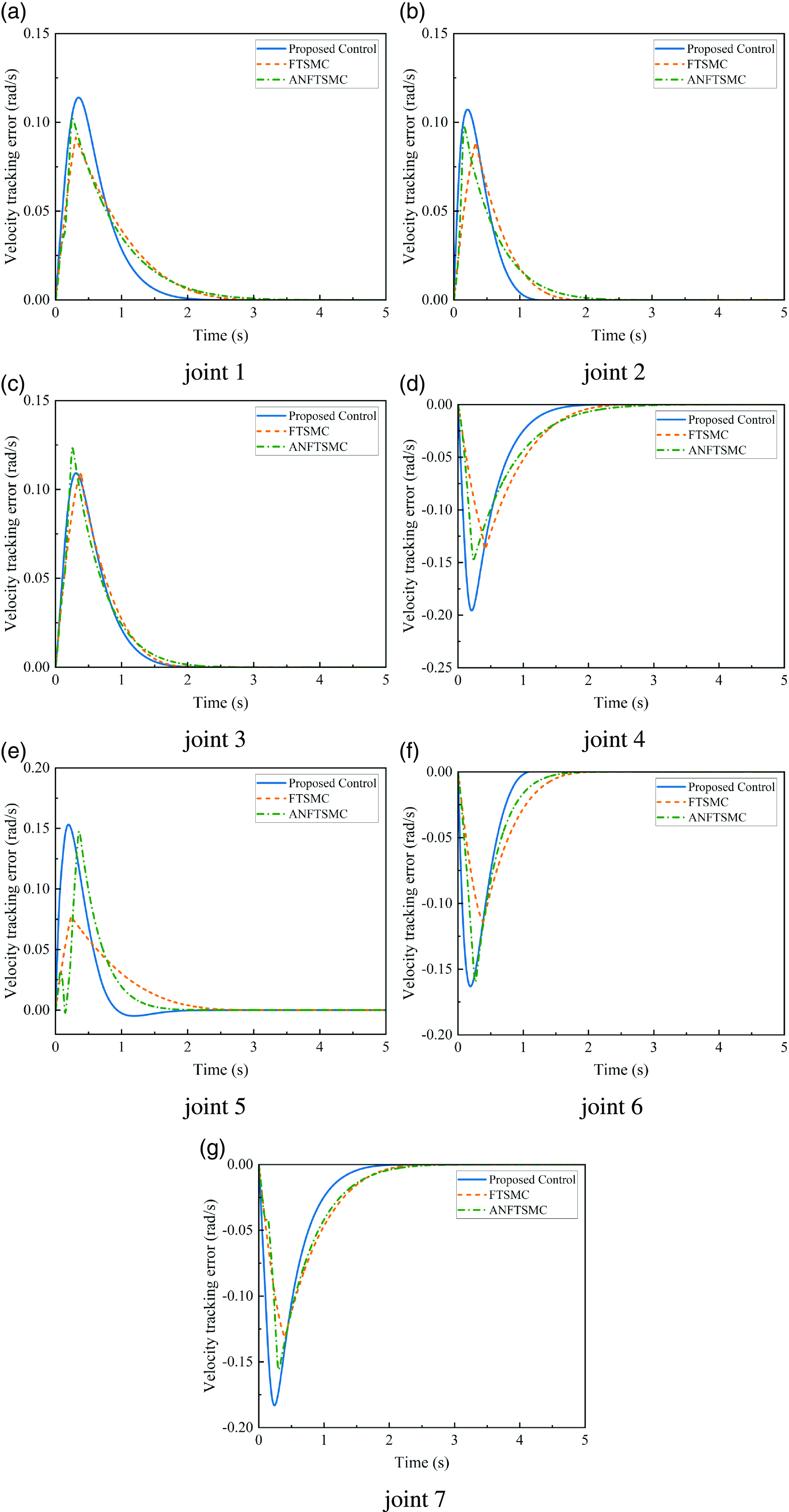
Figure 12. Velocity tracking error performance.
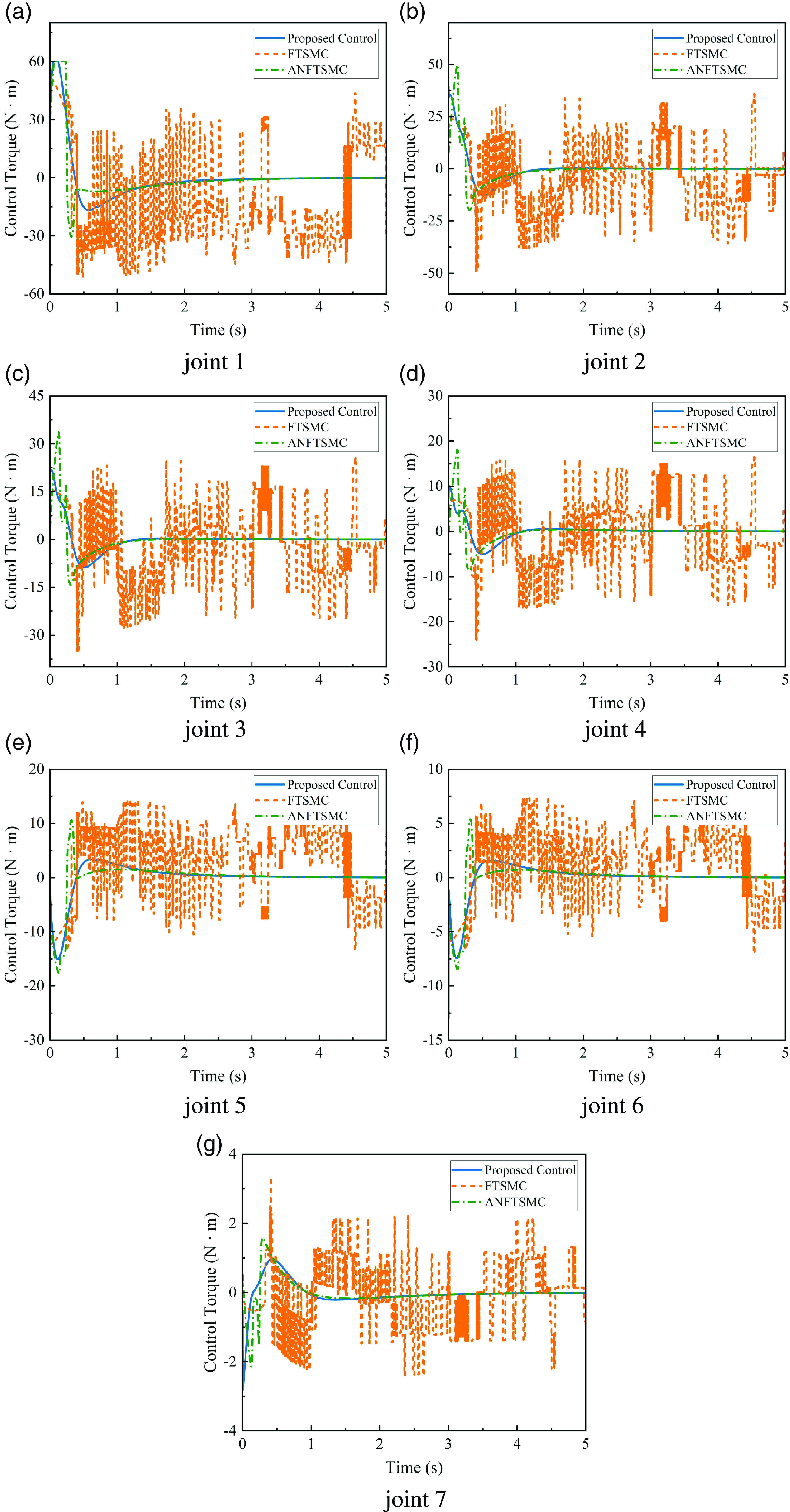
Figure 13. Control torque.
To quantitatively evaluate the performance of the various controllers, for the total number of sampling times $N$
, three metrics including the integrated absolute error (IAE)
$N$
, three metrics including the integrated absolute error (IAE) ${\rm{IA}}{{\rm{E}}_{{e_{1i}}}} = {1 \over N}\mathop \sum \nolimits_{j = 1}^N \left| {{e_{1i}}\left( j \right)} \right|$
, the integrated time absolute error (ITAE)
${\rm{IA}}{{\rm{E}}_{{e_{1i}}}} = {1 \over N}\mathop \sum \nolimits_{j = 1}^N \left| {{e_{1i}}\left( j \right)} \right|$
, the integrated time absolute error (ITAE) ${\rm{ITA}}{{\rm{E}}_{{e_{1i}}}} = {1 \over N}\mathop \sum \nolimits_{j = 1}^N t\left( j \right)\left| {{e_{1i}}\left( j \right)} \right|$
, and the energy consumption (EC)
${\rm{ITA}}{{\rm{E}}_{{e_{1i}}}} = {1 \over N}\mathop \sum \nolimits_{j = 1}^N t\left( j \right)\left| {{e_{1i}}\left( j \right)} \right|$
, and the energy consumption (EC) ${\rm{E}}{{\rm{C}}_{{u_i}}} = {1 \over N}\mathop \sum \nolimits_{j = 1}^N \left| {{\tau _i}\left( j \right)} \right|$
are introduced, as shown in Tables 4–6.
${\rm{E}}{{\rm{C}}_{{u_i}}} = {1 \over N}\mathop \sum \nolimits_{j = 1}^N \left| {{\tau _i}\left( j \right)} \right|$
are introduced, as shown in Tables 4–6.
Table 4. IAE index comparison of different controllers
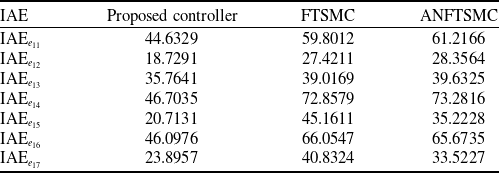
Table 5. ITAE index comparison of different controllers
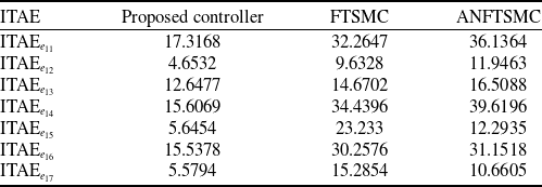
Table 6. EC index comparison of different controllers
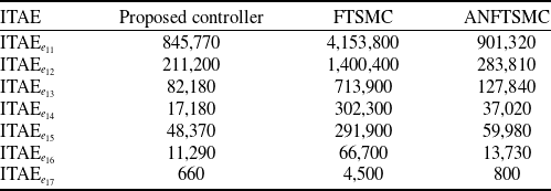
The lower the values of the above three indicators, the better the control performance of the closed-loop tracking system. According to the comparison, the proposed control method can achieve faster tracking convergence and higher tracking precision with less energy consumption than the other two referenced methods. The simulation results demonstrate the noticeable superiority of the proposed controller in terms of tracking performance, energy consumption and chattering suppression.
In summary, it can be concluded that the proposed controller realises fast and accurate trajectory tracking of the space manipulator in a bounded time, while satisfying the transient and steady-state performance constraints of tracking error, even in the presence of unknown disturbances, inertial uncertainty and input saturation.
5.0 Conclusion
The tracking control issue for a free-floating space manipulator with prescribed performance constraints was addressed in this study, along with an efficient solution taking into account model uncertainties, internal disturbances and input saturation. A novel tangent-type PPC integrated fast fixed-time terminal sliding mode control was developed to prevent any violations of the tracking error constraint. To offset the negative effects of excessive actuator torque, an input compensator was introduced. The suggested controller is not only straightforward structurally, but also capable of guaranteeing fixed-time prescribed performance fulfillment even in the presence of input saturation. Compared with the existing fixed-time controllers, the designed control has the advantages of faster convergence rate, higher tracking precision and less control torque chattering. It is important to note that measurement noise, which deteriorates system tracking performance, is not taken into account in this research. More research needs to be undertaken with measurement noise explicitly considered in future work for tracking control of a space manipulator.
Competing interests
The authors declare that they have no Competing of known competing financial interests or personal relationships.


