


1. Introduction
Public and occupational pension reforms have been on the Organisation for Economic Co-operation and Development (OECD) policy agenda for decades. One particular concern is the increase in the dependency ratio of older adults from 20.6% in 1990 to 31.2% in 2020, with projections of 53.4% for 2050 (OECD, 2019).Footnote 1 In response to such increases in their dependency ratios, most OECD countries have introduced changes in their pension systems in an effort to improve their financial sustainability. The challenge is to ensure the sustainability of pension systems without damaging the social safety net of the elderly. Public pensions play an important role in seniors' financial health (OECD, 2019, Chapter 7). Thus, in this context, it becomes very important to study the financial consequences of retirement, and more specifically, the role of public pensions, on the financial well-being of older individuals.Footnote 2
Research has also shown that average lifetime earnings and the level of integration in the labour market during work years are important for explaining poverty dynamics (see, for instance, Valetta, Reference Valetta2006, Biewen, Reference Biewen2009, Hansen et al., Reference Hansen, Lofstrom, Liu, Zhang, Carcillo, Immervoll, Jenkins, Königs and Tatsiram2014, among others). This literature focuses on the entire population, but it is an important first step in understanding the determinants of older adults' poverty. In this line, Finnie et al. (Reference Finnie, Gray and Zhang2013) find that in Canada, the probability of having a low level of income at 65 is strongly associated with individuals' past level of permanent income. Another strand of the literature has investigated the relation of public pensions on poverty among the elderly. For instance, Engelhardt and Gruber (Reference Engelhardt and Gruber2004) highlight the important role that Social Security has had in reducing U.S. poverty rates. More recently, Engelhardt et al. (Reference Engelhardt, Gruber and Kumar2020) analyse the impact of claiming early pension benefits on the poverty rate among old-age individuals. Our paper is motivated by both strands of the literature, which has highlighted that the financial well-being of older adults is determined both by their labour market opportunities and by social safety nets provided by the welfare system.
In particular, our paper identifies the role of public pensions in alleviating poverty among senior Canadians. We pay particular attention to the relation of public pensions on poverty dynamics, i.e., whether they reduce the probability of entry into poverty or increase the probability of exit from it. To understand whose risk of poverty is affected most by public pensions, we also analyse how lifetime earnings affect individuals' old age financial well-being. Moreover, we also analyse the association of public pensions on poverty at senior ages by taking into account the unobserved heterogeneity of individuals using a state dependence model and taking into account past earning history.
While there is literature on poverty among Canadians at older ages, previous research did not focus on the role of public pensions and poverty dynamics taking into account the individuals' lifetime earnings. Canada has experienced an important decline in poverty among the elderly since the seventies. Heisz (Reference Heisz2015) shows that the poverty rate for those aged 65 and over decreased from 30.4% in 1977 to 5.2% in 2011 when using an absolute measure (called LICO: the low-income cut-off poverty measure). With an alternative relative measure (called LIM: low-income measure)Footnote 3, the poverty rate similarly fell to a low of 3.9% in the mid-nineties, only to subsequently increase once more. Several studies have argued that this decline occurred as a consequence of the expansion of public and earnings-related pensions, which reduced poverty rates among seniors (see Kangas and Palme, Reference Kangas and Palme2000, Osberg, Reference Osberg2001, Myles, Reference Myles2010, among others). But these studies base their conclusions on time series trends in aggregate data. When surveying the studies that approach the question using micro data, it becomes apparent that most of them also focus on the evolution in time of poverty rates following the increase in generosity of the public pension system (such as Milligan, Reference Milligan2008, Veall, Reference Veall2008, Schirle, Reference Schirle2013, among others).
We use recently released individual-level data with an administrative data component, the Canadian Longitudinal and International Study of Adults (LISA). This dataset allows us to observe individuals for a period of more than a decade (2001–2016), with very accurate measurements of income, and enables us to distinguish in detail among different types of pension income thanks to the administrative data. We are therefore able to estimate the relationship of receiving public pension benefits on poverty dynamics as well as on the risk of poverty. Finally, the unique combination of survey and administrative data allows us to combine the administrative information with information typically only available in surveys, such as detailed demographic characteristics and life events. Relative to existing research, our main contributions thus are (i) to show how information on past earnings and poverty can help us understand the current situation of seniors living in poverty, (ii) to analyse of the impact of changes in the family structure and employment status on poverty transitions and persistence among older adults and (iii) to determine the state dependence and the persistence of poverty among older adults in a dynamic model taking into account unobserved heterogeneity of individuals.
Our results show that poverty among seniors is highly persistent, i.e., exit rates from poverty are lower than among younger individuals, while poverty spells last longer. Entry into poverty is driven by health shocks, job loss or marital separations, with health shocks being relatively more important for older individuals. Our key findings show that for those individuals over 50 who enter poverty, receiving public pension benefits is crucial for avoiding poverty later on in life, because these benefits increase the probability of exiting poverty. Therefore, public pension benefits help to explain the lower overall incidence of poverty among older adults. By estimating a dynamic probit model and controlling for individuals' unobserved heterogeneity, we are able to measure the importance of state dependence and persistence for older adults. Moreover, we present new evidence showing that individuals with low past average earnings during their careers have a higher probability of being poor when they are older than 65. While public pensions do not completely eliminate poverty among older adults, they do help to alleviate it by reducing persistence and increasing exit.
This paper is structured as follows. Section 2 summarizes related literature on poverty among the elderly, on the role of lifetime earnings and on Canadian public pensions and poverty. Section 3 describes the data and the main variables, with stylized facts on poverty. Section 4 estimates the role of public pensions on poverty at older ages. Section 5 estimates whether public pensions affect the probabilities of entry into and exit from poverty. Section 6 analyses the results with a dynamic random effects model. Finally, Section 7 offers a conclusion.
2. Related literature: public pensions and poverty
In this section, we first highlight the most relevant studies on poverty at older ages and on the role of lifetime earnings. We then describe results on Canadian public pensions and poverty that are important in the context of this research.
At the international level, a significant part of the literature on income and poverty among the elderly has focused on analysing the relationship between different pension systems and economic well-being. Indeed, several studies have confirmed the negative relationship between public pension spending and the probability of being poor among the elderly at the aggregate level (see Lefebvre and Pestieau, Reference Lefebvre and Pestieau2006, Jacques et al., Reference Jacques, Leroux and Stevanovic2021). At the micro level, other cross-sectional and cross-country studies such as those of Smeeding (Reference Smeeding2006) and Smeeding and Williamson (Reference Smeeding and Williamson2001) have also associated public pension spending to the alleviation of poverty at older ages. Zaidi et al. (Reference Zaidi, Grech and Fuchs2006) find similar results. Fonseca et al. (Reference Fonseca, Lee, Zamarro, Zissimopoulos, Frechet and Gauvreau2011) also find that being older than key public pension cut-off ages makes people less likely to be poor in continental Europe, the United Kingdom, and to a lesser extent, the Unites States.
Results from several previous studies have pointed out the importance of poverty dynamics to understand the determinants of poverty (see, e.g., Antolín et al., Reference Antolín, Dang and Oxley1999; Oxley et al., Reference Oxley, Dang and Antolin2000, for different countries).Footnote 4 They find that poverty is more likely to recur for some individuals.Footnote 5 In a cross-country analysis, Valetta (Reference Valetta2006) finds that the poverty persistence is higher in North America than in Europe. In particular, for the period 1993–98, Canada had a high share of chronically poor individuals relative to those who were ever poor. Biewen (Reference Biewen2014) finds that looking at the poor in only one period provides an incomplete picture of poverty because a considerable part of the measured poverty is transitory rather than persistent. Closer to our analysis for Canada, Finnie and Sweetman (Reference Finnie and Sweetman2003) using administrative data covering the period 1992–96, for example, find a strong ‘occurrence dependence’ for poverty entry and incidence, while Hansen et al. (Reference Hansen, Lofstrom and Zhang2006) and Hansen et al. (Reference Hansen, Lofstrom, Liu, Zhang, Carcillo, Immervoll, Jenkins, Königs and Tatsiram2014) find that endogenous initial conditions and unobserved heterogeneity play an important role in explaining social assistance participation. They use longitudinal data for the period 1993–2010. In contrast to this literature, we concentrate on older ages and examine the public pension claiming. In fact, Engelhardt and Gruber (Reference Engelhardt and Gruber2004) find for United States, that adjusting public pensions is a direct policy intervention capable of impacting the financial well-being of seniors, as well as reducing poverty rates among seniors. Engelhardt et al. (Reference Engelhardt, Gruber and Perry2005) predict that a cut in Social Security benefits would cause more elderly households to move into shared living arrangements. Recently, Engelhardt et al. (Reference Engelhardt, Gruber and Kumar2020) analyse the impact of early pension benefits claiming for the 1885–1916 cohorts, and find that the early claiming is related to an increase in the poverty rate in old male aged individuals. Our study shows that one particularly important aspect of poverty among the older adults is its persistence, and we carefully take that into account in our analysis by considering lifetime earnings of individuals.
Canada is a pay-as-you-go (PAYGO) pension scheme with partially funded public pensions for workers. In this paper, we define public pensions as the sum of the Old Age Security (OAS), the Guaranteed Income Supplement (GIS), and the Allowance.Footnote 6 There is also a public partially funded Canada/Quebec Pension Plan (CQPP) for workers that we do not include in our definition of public pension and that we exclude from our main analysis.Footnote 7 We provide a more detailed explanation of the pension system in Canada in Appendix A.
Several studies have investigated the relationship between pension system reforms and the alleviation of poverty among the elderly in Canada (see Kangas and Palme, Reference Kangas and Palme2000, Osberg, Reference Osberg2001, Myles, Reference Myles2010, among others). Osberg (Reference Osberg2001) and Myles (Reference Myles2010) both argue that the introduction of the OAS in 1952 and GIS in 1968 as well as the maturing of the CQPP regimes established in 1966 contributed to alleviating poverty among the elderly since the beginning of the seventies. Osberg (Reference Osberg2001) considers the reduction of poverty among senior citizens as being the major success of Canadian social policy in the twentieth century.Footnote 8 Myles (Reference Myles2010) also claims that these reforms have helped reduce income inequality among seniors, since they benefited lower-income individuals more than anyone else. Kangas and Palme (Reference Kangas and Palme2000) examine to what extent poverty cycles along the individual's life are still apparent in OECD countries (including Canada). In most countries, poverty among the elderly has declined, and the young have replaced the old as the lowest income group. Our study will not focus on pension reforms but on how claiming public pension affects the probability of having a low-income status.
Other studies using micro data, such as Schirle (Reference Schirle2013), Milligan (Reference Milligan2008) and Veall (Reference Veall2008), similarly relate the evolution of poverty among the elderly to the increase in generosity of the public pension system and to variation in income growth over time. In particular, Milligan (Reference Milligan2008) computes several measures of poverty among the elderly and studies their evolution during the period 1969–2004 with several datasets; the Survey of Consumer Finances (SCF), and the Survey of Labour and Income Dynamics (SLID). He finds that incomes of the elderly have grown more rapidly than those of the working-age population from 1973 to 1990. Poverty rates have been constant afterwards, although some relative measures of poverty increased after 1997, as also seen in Heisz (Reference Heisz2015). This could reflect the interaction between the evolution of pensions and gains in income in other groups of the population. In fact, Baker et al. (Reference Baker, Gruber and Milligan2009) show that individuals adjust their behaviours, such as employment and savings, based on expected retirement conditions. In a study of 19 countries, Fonseca et al. (Reference Fonseca, Kapteyn, Lee, Zamarro and Feeney2014) also find that individuals with a higher risk of poverty tend to opt for earlier retirement. Finnie et al. (Reference Finnie, Gray and Zhang2013) use the Longitudinal Administrative Database (LAD) to analyse a related question about the probability of receipt low-income support benefits (GIS) when 65, and they find that this is strongly associated with individual's past level of permanent income.
Bernard and Li (Reference Bernard and Li2006) and Veall (Reference Veall2008) also use data from LAD to describe poverty among seniors in Canada. Bernard and Li (Reference Bernard and Li2006) focus on the impact of the death of the spouse, and find that this can affect poverty rates because there is a reduction in the public pension receipts (for instance, OAS and GIS). Veall (Reference Veall2008) compares relative poverty rates for groups of seniors with different characteristics, e.g., by living arrangement or immigrant status, and relate their results to the design of public pension plans, in order to understand which adjustments to the pension system (e.g., increasing GIS benefits for single persons) would be most effective at helping seniors exit poverty. In contrast to our study, these previous studies, however, base their conclusions on time series trends or aggregated characteristics.
The present paper differs from the above-mentioned studies by analysing the association of individuals receiving public pension benefits on the probability of being poor, entering or exiting poverty, and by using dynamic econometric models to analyse poverty at the micro level taking into account past earning history and/or unobserved heterogeneity.
3. Data and stylized facts
In our analysis we use three waves of LISA: wave 1 (2012), wave 2 (2014) and wave 3 (2016). LISA is a longitudinal survey conducted every 2 years by Statistics Canada that contains information on individuals' income, health status and demographics (such as education or marital status).Footnote 9 The data have been linked with administrative data sources (T1 and T4 files) starting from 1982. This retrospective component of the data is particularly important for this analysis, since it allows us to study how changes in individuals' earnings are related to poverty entry, exit and persistence for older adults. Only starting from 2001, the dataset provides a measure of relative poverty calculated at the level of the census family. Since we are interested in using this measure, we will restrict our analysis to the period 2001–16.
In our analysis, we mainly use the LIM which is a relative poverty measure depending on a given income distribution.Footnote 10 LIM is defined as a fixed percentage (50%) of the median adjusted household income. However, for robustness, we also use two absolute measures of poverty: the LICO and the market basket measure (MBM)Footnote 11 for the period after 2012.Footnote 12 The absolute measures of poverty consider poverty to be a situation of income deprivation that does not depend on the income distribution in a society.Footnote 13 The adjustment for family size is meant to reflect the fact that a household's needs increase as the number of members increase, although not necessarily proportionally.
Since we do not have information on the household size and labour status in the retrospective component of the administrative data, we can only compute the poverty measures for the survey years 2012, 2014 and 2016. On the other hand, as mentioned above, the dataset provides the LIM from 2001 using the census family adjustment. Therefore, the results shown in the main text were computed using the LIM, and when we will include measures of poverty persistence, we will restrict our sample to those years. The LIM provided by LISA uses net income (i.e., after tax and transfers).Footnote 14
Table 1 shows the poverty rates for individuals over 50 using the three previously discussed measures. All measures show that age is an equally important correlate of poverty: poverty rates are lower for those over 65. The first column shows poverty percentages calculated using the LIM. Results change according to which of the three measures we use. For instance, when we use the MBM, the poverty levels are higher. For the MBM, results also change depending on which family unit we use.Footnote 15
Table 1. Poverty rates for individuals 50 or older in Canada using different poverty measures (2012–16)
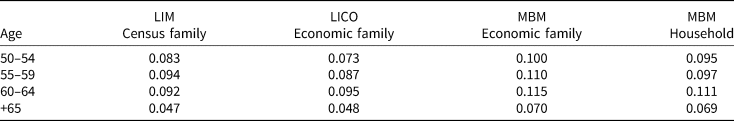
Note: LIM is calculated as the percentage of families with income lower than the 50% of the median income (adjusted by family size). LICO and MBM are calculated using the cut-offs estimated and reported by Statistics Canada. All the rates are constructed using after-tax income.
We have compared different measures of poverty (both relative and absolute). The poverty rates differ. Measures are different in thresholds, as well as in the components of the household income. The levels of poverty also depend on family unit definitions. Note that the economic family or household might in some cases also include other persons apart from the elderly individuals or couple, for example adult children or other adults living in the same household.Footnote 16 Since the administrative data only provide the historical LIM variable at the level of census family, we use results for census families throughout. The rest of the paper will use this measure, unless we specify otherwise.
In Table 2, we break down poverty statistics by individual and family characteristics. Note that in Table 2, as well as the following tables, we adopt the LIM as our primary measure. The results show that levels of poverty are lower for men, for individuals with higher levels of education, for those who self-report having an excellent or very good health, and for those living with a partner. They are higher for lone parent families,Footnote 17 which are mostly headed by women.Footnote 18 The poverty rates of the elderly shown in Table 2 are in line with those found by Smeeding and Weaver (Reference Smeeding and Weaver2002) using data from the Luxembourg Income Study. These authors also show that the poverty rate in Canada is substantially lower than that in some other countries, in particular the United States, Australia and the United Kingdom, and lies between those in Continental European and Scandinavian economies.
Table 2. Summary statistics: poverty rates by demographic group, individuals 50 or older (2012–16)
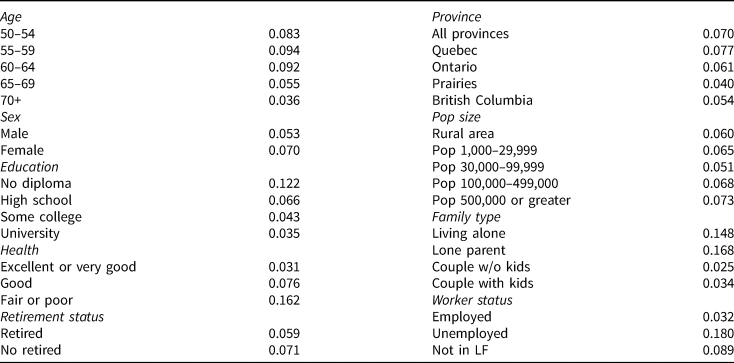
Note: Retirement status and health are self-reported. Population size refers to the size of the place where the family lives. Family type refers to the type of census family. Four different options are possible: a married couple and the children, if any, of either and/or both spouses; a common law couple and the children, if any, of either and/or both partners; or a lone parent of any marital status with at least one child living in the same dwelling and that child or those children.
The poverty rate for those who are unemployed at the time of the survey is high, at 18%. In particular for middle aged and older individuals, whose unemployment spells last longer, unemployment implies a substantial hit in income, putting them at risk of poverty. Table 2 also shows that there are no important differences in poverty rates by retirement status (self-reported).Footnote 19
There are different ways to account for poverty persistence.Footnote 20 In the present paper, we use the number of years spent in poverty in the past as a continuous measure indicating the degree of poverty persistence for an individual. We also account for both the number of poverty spells and the length of these spells (see Appendix Tables C.1 and C.2).Footnote 21
In addition, we use what has been called an ‘at-risk-of-poverty’ measure. This measure considers a person who was poor in a given year, and in at least two of the three preceding years, to be persistently poor. Moreover, we account for the ‘average-income poverty’, computing the past average earnings of the individual. Since we can estimate 14 years, we will use this information in our regressions as an estimate of permanent income.Footnote 22
4. Relation of public pensions on poverty persistence among older adults
4.1 Prevalence of poverty among older adults
We use a probit model to estimate the probability of being poor as a function of different characteristics that were found relevant and were documented in the literature on poverty at older ages. However, since cohorts may differ in their characteristics – older cohorts, for example, have systematically lower levels of education – it is important to verify that the differences in the incidence and persistence of poverty documented above are not driven by these confounding variables. Table 3 shows marginal effects from these regressions. We include different variables in the regression: socio-demographic factors, labour market arrangements, living arrangements and health outcomes. The retired dummy controls for whether a respondent is completely retired. For these regressions, we pool the data for 2012, 2014 and 2016.
Table 3. Probability of being poor conditional on demographic characteristics (2012–16)
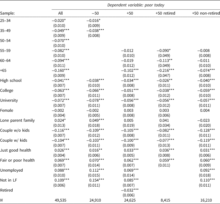
Note: We have estimated a probit model where the dependent variable is an indicator function that takes the value one if the individual lives in a poor family (defined as having an income below 50% of the median income adjusted by census family size). The base category corresponds to a male head of the household who is 15–24 years old, has no diploma, is living alone, reports having an excellent or very good health, is employed and therefore not retired. For those columns where the sample has been restricted to individuals over 50 years old, the base category corresponds to heads of the family who are 50–54 years old. Clustered standard errors are reported in parentheses. ***Significant at less than 1%; **significant at 5%; *significant at 10%.
In the first column of the table, we pool all age groups. The results indicate that the probability of being poor is significantly lower for individuals 35 and older compared to individuals 34 and younger. The probability of being poor, already lower for those between 35 and 49, declines even further for those aged 50–64, and even more for those over 65. The coefficients on most of the other demographics are in line with the bivariate results shown in Table 2. Each additional level of schooling reduces the probability of poverty. For individuals who live alone, having children is associated with a greater incidence of poverty. This is not the case for couples. In addition, couples have a lower incidence of poverty compared to single households, no matter the number of children. Fair or poor health (as opposed to good, very good or excellent health) is associated with a higher incidence of poverty. Finally, the unemployed and those not in the labour force are also noticeably more likely to be poor.
The remaining columns show results for the same regression, broken down by age category (50 years old and above or below) and retirement status. Qualitative results are very similar, but point estimates differ. For instance, we see that the higher risk of poverty for lone parent families is driven by those under 50. While the effects of unemployment and non-participation on the incidence of poverty are higher for younger individuals, they remain substantial for those above 50. Finally, those who are retired are significantly less likely to be poor. Clearly, the results on retirement cannot be interpreted as causal given that retirement is a choice, meaning that, for example, people may choose to work longer if retirement would imply poverty, or to claim early pension benefits and retire earlier if that meant a comfortable living standard.
4.2 Persistence of poverty
We now analyse the probability of being poor controlling for demographics and for time spent in poverty. These regressions use data for 2014 only and we compute for how long the individual has been poor between 2001 and 2013. We define the variable ‘years poor’ as the length of the ongoing spell of poverty for those who are poor in 2014. We then group individuals depending on whether this spell was 1 year long, 2 to 3 years long or 4 or more years long. Table 4 (panel A) shows the marginal effects of these categorical variables on 2014 poverty status. It reports a much higher probability of being poor in 2014 for those who were previously already poor, thus showing that poverty is persistent. When considering all age groups, the probability of being poor in 2014 increases with the length of an ongoing poverty spell. In other words, those who have been poor for some years already are more likely to remain poor, and the longer the poverty spell, the more likely they are to remain poor. This corresponds to a declining hazard for exit from poverty.
Table 4. Probability of being poor conditional on demographic characteristics – controlling for time spent in poverty and for past average earnings
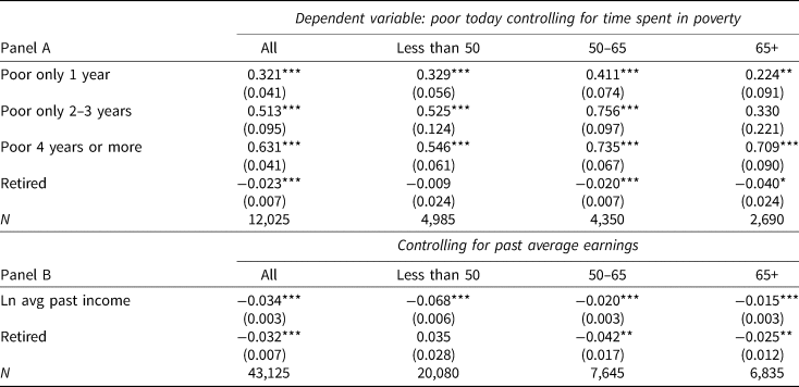
Note: For the exercise shown in panel A we use data from 2014 only, in Panel B we use data for 2012–16. We have estimated a probit model where the dependent variable is an indicator function that takes the value one if the individual lives in a poor family (defined as having an income below 50% of the median income adjusted by census family size). All these regressions control by education, household composition, self-reported health, labour market status and a dummy that indicates if the individual is retired. In column 1 we also include age dummies. In columns 2–4 we separate the sample based on the age of the head of the household. Age is then not included in the regression. The base category corresponds to a male head of the family who is 15–24 years old, who has no diploma, is living alone, reports having an excellent or very good health, is employed and therefore non-retired. In panel A, we include as explanatory variable an indicator function that takes the value one if in the last 14 years the family has been poor only 1 year, only 2 or 3 years or 4 years or more. In panel B we include the log of the average past income. Clustered standard errors are reported in parentheses. ***Significant at less than 1%; **significant at 5%; *significant at 10%.
Table 4 (panel B) shows the link of past average earnings on the probability of being poor.Footnote 23 Results show that past average income is a powerful predictor of current poverty status. This is in line with previous work done in other contexts which has shown that individuals who have spent more time in poverty are more likely to be poor at any given moment.Footnote 24
These results suggest that for older adults, current poverty is closely related to prior experience of poverty. Figure 1 shows the distribution of average earnings over a career (25–64 years of age) for the individuals in our sample. We show the distribution separately for the poor (panel a) and the non-poor (panel b). Poor seniors on average had career earnings that were $18,600 per year lower than the non-poor. Among the poor older adults, 50% had average yearly career earnings below $10,600, compared to 16% among the non-poor.
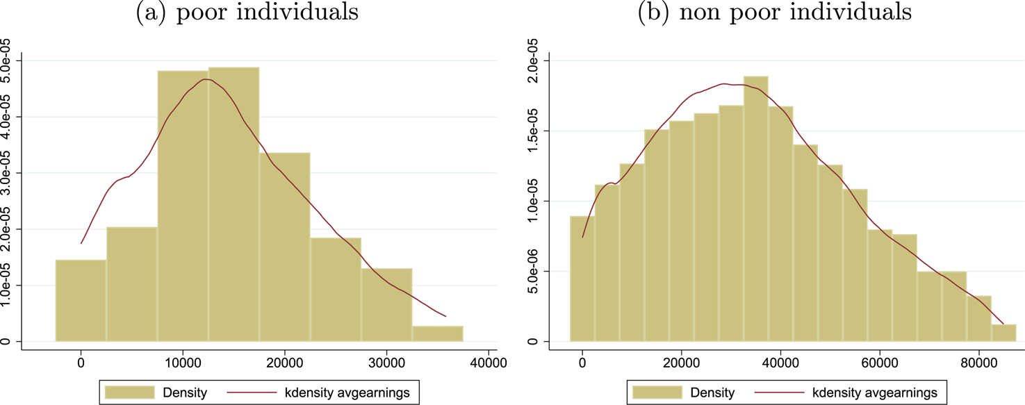
Figure 1. Distribution of average earnings over a career (25–64 years of age).
Note: We use individuals older than 65 in 2014. Annual earnings expressed in 2011 dollars, adjusted using the CPI, and smoothed using a nonparametric lowess estimator. Source: Statistics Canada and authors’ calculations.
To summarize, older people are less likely to be poor. At the same time, poverty is highly persistent for them, and therefore they have a high probability of undergoing a long spell of poverty if they are ever poor.
This is in line with the relationship between career earnings and the risk of poverty.
4.3 The Role of public pensions in reducing poverty among older adults
Although we have shown that poverty rates and risk of poverty are lower among older individuals, in particular those over 65, we have also shown the persistence of poverty at those ages. Previously cited literature shows the importance of the role of public pensions in reducing poverty at senior ages. In this section, we investigate the extent to which the public pension system drives these findings.Footnote 25 To do so, we use the same model as in Table 3 including a dummy that indicates if the head of the householdFootnote 26 is receiving a public pension. To identify the link of public pensions with poverty independently from age, we use the variation in the timing of receiving public pensions. We do not exploit policy changes or variation in the generosity of the pensions, but we exploit the fact that not all individuals start receiving a public pension at the age of 65. These cases represent more than 7% of our sample. Some claim the allowance and the allowance for the survivor when they are between 60 and 64 years old. Household heads under 65 may also report receiving a public pension if the partner is over 65 years old. Others are not eligible for public pension benefits, as is the case of immigrants who lived in Canada for less than a decade since they turned 18, or individuals with incomes above a certain threshold.
We also include an interaction of the interaction term between receiving public pension and the dummy retired to understand better the relationship between receiving a public pension and poverty. Our hypothesis is that this relationship can be stronger for individuals without labour income because of retirement. We will also take into account in our specifications the number of years being poor or the past average earnings for the period 2001–16.
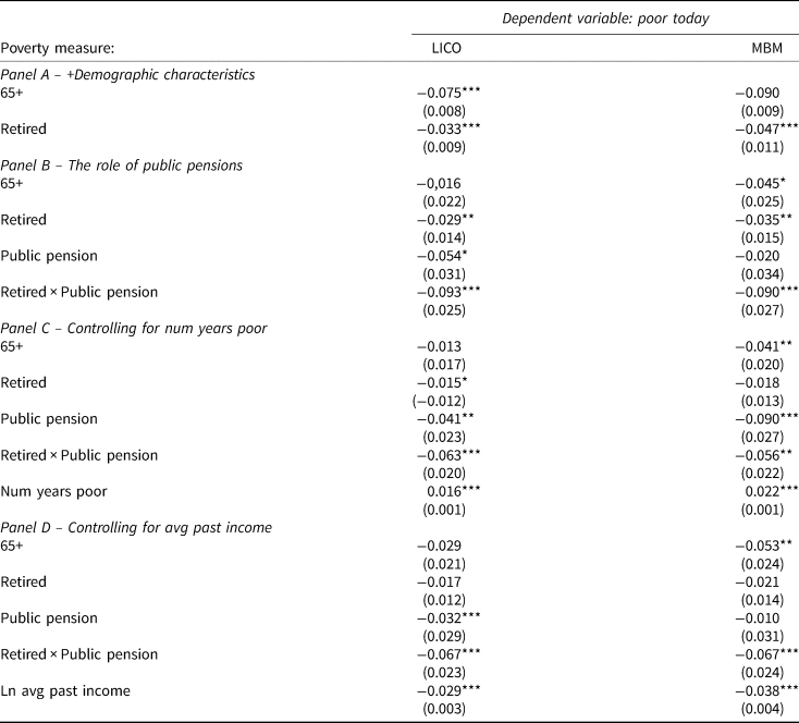
Results are shown in Table 5, column 2. Receiving a public pension reduces the probability of being poor by 13%. In columns 3 and 4 we perform the same exercise, but now we control for the number of years spent in poverty just before the survey year (our measure of persistence) as well as the logarithm of average past earnings. Results indicate a strong interrelation of past poverty on the risk of poverty today. The risk of poverty is also closely related to career earnings. In all of these specifications, the relation of public pensions on the risk of poverty is negative and significant. Controlling for past average income (column 4), for someone who is not retired, receiving public pensions reduces the probability of being poor by 8%. The coefficient associated with the interaction between public pensions and retirement is negative, indicating that the effect of public pensions is stronger for those who do not receive labour income.
Table 5. The role of public pensions on the probability of being poor controlling for persistence and past average earnings
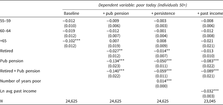
Note: For this exercise we use data for 2012–16. We have estimated a probit model where the dependent variable is an indicator function that takes the value of one if the individual lives in a poor family (defined as having an income below 50% of the median income adjusted by census family size). All these regressions control by education, household composition, self-reported health and labour market status. The base category corresponds to a male head of the household who is 50–54 years old, who has no diploma, is living alone, reports having an excellent or very good health, is employed and non-retired and not receiving public. Clustered standard errors are reported in parentheses. Nb yrs in poverty measures the number of years that the individual has been poor during the period 2001–11. ***Significant at less than 1%; **significant at 5%; *significant at 10%.
For robustness, we also analyse not only how ‘universal’ pension income,Footnote 27 but also income-linked pensions affect the risk of poverty. For most pensioners, the main component of their pension consists in payments from the Canada and Quebec Pension Plans (CQPP), which are a function of lifetime earnings. Those are supplemented by payments from public pension plans (except for high-income earners). To analyse their interaction, we add to the previous model a full set of dummies and interactions of indicator variables for retirement, public pension receipt and CQPP pension receipt.Footnote 28 Results are shown in Table C.3 in Appendix C. CQPP and public pension receipt are both associated with a significantly lower risk of poverty.Footnote 29
Who are those for whom public pensions make the difference? Until now we have seen that, for many old people, poverty is persistent and associated with their characteristics, namely lower labour market participation, a higher probability of unemployment, lower levels of education and worse health. We have also seen that public pension benefits can play an important role in reducing poverty at older ages.
We want to investigate more closely for which individuals these benefits have the most important effect in terms of reducing the risk of poverty. To do so, we again regress poverty status on individual characteristics, but now interact the dummy ‘presence of public pension’ with the past average income of the individual. We repeat this regression by interacting the dummy ‘presence of public pensions’ with the amount of CQPP income.
Figure 2 shows the marginal effects of the variable ‘presence of public pensions’ evaluated at different levels of the individual career average income. Results in Figure 2a are obtained from regressing poverty status on individual characteristics similar to Table 3, but adding an interaction of the dummy ‘presence of public pension’ with the past average income of the individual. Results from Figure 2b are obtained from a similar regression but adding CQPP as a control variable. It is very clear from the figures that public pensions have the strongest negative association on the risk of poverty for individuals with average career incomes below $30,000, and when controlling for CQPP, income below $20,000. For example, receiving benefits does not reduce the risk of poverty in a statistically significant way for individuals with average career income of $50,000, while it reduces it by 20 percentage points for individuals with average career income of $10,000. This occurs because individuals with high career earnings tend to have more resources as they get older, including higher pensions, and therefore are hardly at risk of poverty to begin with. Individuals with low career earnings have fewer resources, so that receipt of a public pension can significantly reduce their probability of being poor.
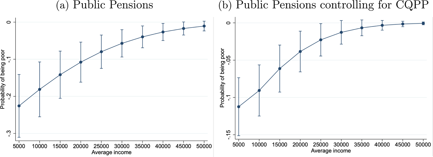
Figure 2. Heterogeneity in the relation of public pensions on the probability of being poor.
Note: Panel (a) shows the relation of public pensions on the probability of being poor as a function of average earnings over a career. We run a regression of poverty status on individual characteristics (as in Table 3), adding an interaction of the dummy ‘presence of public pension’ with the past average income of the individual. Panel (b) shows the relation of public pensions on the probability of being poor as a function of average earnings over a career controlling for the presence of the CQPP. We run the same regression as in panel (a) but controlling for the presence of CQPP. For these regressions we restrict the sample to individuals over 50 in 2014. The figure shows marginal effects of the interaction, evaluated at different levels of average career income and 95% confidence intervals. Annual earnings are expressed in 2011 dollars, adjusted using the CPI. Results reported are for an individual who is a male head of the household, younger than 65, has no diploma, is living alone, reports having an excellent or very good health, is employed and therefore non-retired. The bands show the 95% confidence interval of the estimates.
We repeat the analysis using different measures of poverty. Instead of the LIM used above, we use the LICO and the MBM.Footnote 30 Results are shown in Table C.6 in Appendix C. Results generally are qualitatively similar. For the sake of brevity, our discussion here focuses on the role of age and public pensions.Footnote 31 The relation of public pension is negative but not always significant when using the MBM. However when we control for the interaction between retirement and public pension benefits, the probability of being poor decreases for all measures. The magnitude of the coefficients associated with the number of years spent in poverty and past income do not vary much across the different measures.Footnote 32
5. Do public pensions help to exit poverty?
The previous section focused on the incidence and duration of poverty spells. These quantities are, in turn, determined by flows in and out of poverty.
In this section, we analyse how these flow probabilities depend on age and individual characteristics, in particular the role of receiving public pension benefits. Since entry and exit may be triggered by other events, we also include life events that occur in the year of poverty entry or exit.
The data allow defining the following events: becoming a widow or a widower, divorcing, forming a couple, worsening and improving health, entering unemployment or finding a job, retiring and beginning to draw a pension. We estimate probit regressions using data for 2012, 2014 and 2016. For the regressions on exit, the sample consists of individuals who were poor in 2012 or in 2014, and the dependent variable is an indicator variable that takes the value one if they were not poor in 2014 or in 2016 respectively, and zero otherwise. That is, a value of one denotes exit from poverty. We also use the past information of the individual from 2001 to calculate the number of years spent on poverty and the average past earnings as defined in previous sections. Definitions are analogous for entry.
Results of marginal effects of the probit regressions for exit from poverty are reported in Table 6. This table shows that employment, higher education and health improvements, lead to increases in the exit rate. Entering retirement is associated with a lower probability of exiting. Column 2 also shows that receiving public pension benefits significantly affects the exit probability. Beginning to draw from a public pension programme is associated with a much larger exit rate from poverty, it increases the probability of exiting by 23%. The probability of exit is also higher for those who are 65 and older compared to the individuals aged 50–54. In columns 3 and 4 we control for the number of years spent in poverty and for past average income measured since 2001. More years in poverty makes one less likely to exit poverty. At the same time, the earnings history of individuals plays a determinant role in their poverty status. Our key variable – receiving a public pension benefit – is still significantly positive. Receiving a benefit increases the probability of exiting by 18–23%. However, when we control for past income and number of years spent in poverty, retirement status becomes insignificant.
Table 6. Poverty dynamics: exit poverty (restricting the sample to individuals 50 and older)
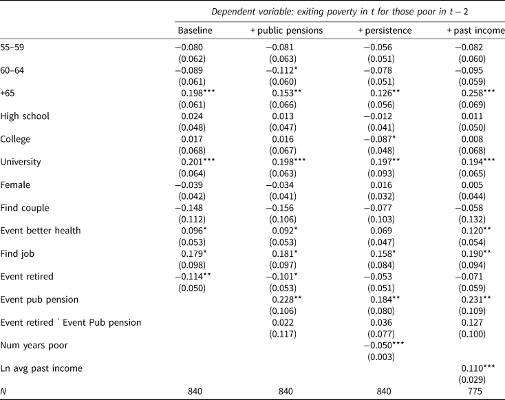
Note: For this exercise we use data for 2012–16 and we restrict the sample to individuals that are older than 50. We have estimated a probit model where the dependent variable is an indicator function that takes the value one if the individual lives in a family that exits poverty (defined as having an income below 50% of the median income adjusted by census family size). The base category corresponds to a male head of the household, who is 50–54 years old, who has no diploma, has not found a couple during the past year, reports not having better health than in the previous period, has not found a job during this period, and has not retired. Clustered standard errors are reported in parentheses. ***Significant at less than 1%; **significant at 5%; *significant at 10%.
For robustness, we also control for the importance of receiving CQPP benefits and we obtain similar qualitative results for the coefficients of receiving public pensions (Table C.4 in Appendix C).Footnote 33
Results of marginal effects for entry to poverty are reported in Table 7. The results of the baseline regression show that entry into poverty is less likely at older ages and for more educated individuals, but more likely for women although the marginal effect is very small. Divorce raises the probability of entering poverty. Job loss and leaving the labour force are both associated with a higher rate of entry into poverty. Finally, receiving public pension benefits does not significantly affect the rate of entry into poverty. Columns 3 and 4 show that the number of years spent in poverty in the past increases the rate of entry into poverty and that higher past average earnings reduce the entry rate into poverty. The relation of receiving public pensions remains insignificant in these settings. For robustness, we also control for the importance of receiving CQPP benefits with similar results (Table C.5 in Appendix C). Interestingly, receiving CQPP benefits decreases significantly the probability of entering poverty.
Table 7. Poverty dynamics: entry into poverty (restricting the sample to individuals 50 and older)
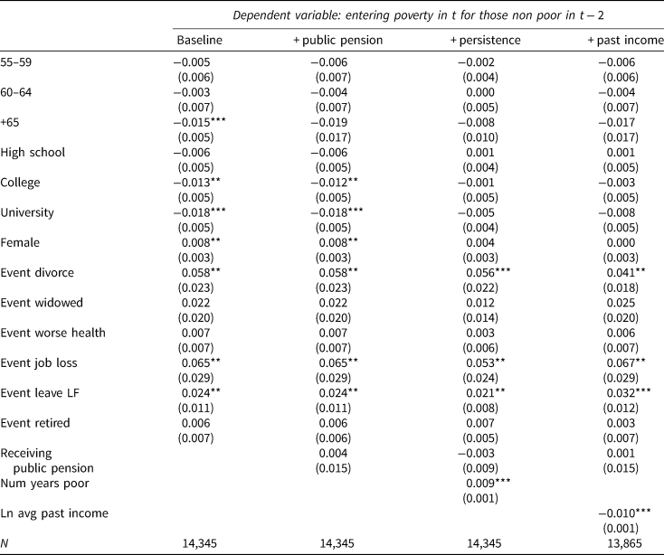
Note: For this exercise we use data for 2012–16 and we restrict the sample to individuals that are older than 50. We have estimated a probit model where the dependent variable is an indicator function that takes the value one if the individual lives in a family that enters poverty (defined as having an income below 50% of the median income adjusted by census family size). The base category corresponds to a male head of the household, who is 50–54 years old, who has no diploma, has not divorced or become widowed during the past year, reports having not having worse health than in the previous period, has not lost the job or left the labour force during the previous year, and has not retired during the previous year. Clustered standard errors are reported in parentheses. ***Significant at less than 1%; **significant at 5%; *significant at 10%.
Figure 3 summarizes the marginal effects of the probabilities of exiting and entering poverty as a function of age. The probability of exit, shown in Figure 3a, peaks at 65. Afterwards, the probability of exit is stable. Figure 3b shows that the probability of entry decreases in age, up to age 65. Past this age, it increases slightly. Older individuals have lower rates of poverty. Although they are less likely to leave it once they enter, the key difference is that their entry rates are lower. Hence, differences in entry rates across age groups dominate those in exit rates in terms of their impact on poverty rates. Given the lower exit rates from poverty for senior citizens, this points to the importance of understanding who among the elderly are poor and why. In terms of poverty exit, public pensions play an important role, but also having a higher average past earnings and fewer years spent in poverty. For entry into the poverty, however, lower past average earnings and more years spent in poverty are very important. Although public pensions do not provide a safety net that prevents poverty entry, in Figure 3b, the probability of entering into poverty is reduced before the normal retirement age of 65.
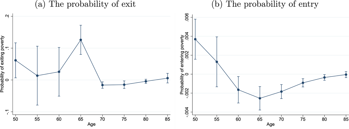
Figure 3. Marginal effect of age on the probability of entering and exiting poverty.
Note: For the left panel, we run a regression on the probability of entering poverty on individual characteristics (as in Table 3), adding age nonlinearly. For the right panel, we run the same regression on the probability of exiting poverty. For these regressions we restrict the sample to individuals over 50 in 2014. The figure shows the marginal effects of age with 95% confidence intervals. Results reported are for an individual who is a male head of the household, younger than 65, has no diploma, is living alone, reports having an excellent or very good health, is employed and therefore non-retired. The bands show the 95% confidence interval of the estimates.
6. Dynamic random effects models
The previous sections investigate the relation between individual and household characteristics as well as public pensions with the dynamics of poverty. In particular, we have modelled poverty dynamics as the probability of exiting or entering poverty conditional on individual characteristics, including receiving public pensions. In some of these specifications we have included proxies for past poverty spells. The probability of exiting or entering poverty in old age may be related to other unobservable and heterogeneous variables that are fixed over time for an individual and that can be correlated with the earnings history, such as ability, motivation or intelligence. The presence of unobservable heterogeneity will affect our parameter estimates. Our analysis in Section 5 aims to capture this heterogeneity via the observed measure of time spent in poverty as well as other observed invariant variables. However, it is also possible that the heterogeneous propensity to be poor in old age is not captured entirely by these variables.
To address this concern, we use a dynamic random effects model, which allows for unobserved heterogeneity in this propensity. In addition, this model separates the effect of past time spent in poverty into that of a recent poverty spell (yielding an estimate of period-to-period persistence of poverty) and a person's fundamental, fixed propensity to be poor. This allows us to estimate how poverty in any given year relates to the probability of being poor in the next year, by accounting for the confounding effect of unobserved heterogeneity in a random effects formulation.Footnote 34
Table 9. Transitions into and out of poverty
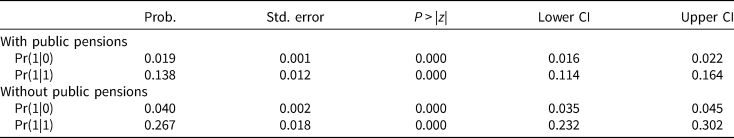
Note: This table shows the transition probabilities calculated with the estimates obtained with the dynamic probit model and presented in Table 8. Pr(1|0) indicates the probability of being poor at time t conditional on not having been in the poor at t − 1. Pr(1|1) indicates the probability of being poor at time t conditional on having been in the poor at t − 1. These probabilities are computed under the assumption of a steady-state Z it = Z i for all t. ***Significant at less than 1%; **significant at 5%; *significant at 10%.
The estimating equation is

where i indexes individuals, and t time. The coefficient ρ captures the risk of poverty in period t − 1, p i,t−1, on the latent poverty variable for period t, p i,t, conditional on a set of time-varying explanatory variables X it. We control both for constant variables like gender and education and for time varying variables like employment status, age groups, marital status, health status and the presence of public pensions. The term c i captures the individual's unobserved characteristics, which are fixed over time, and u it is the idiosyncratic error term. Under the assumption that the unobserved effect c i completely captures unobserved heterogeneity, this approach solves both the problem of unobserved heterogeneity and the initial condition problem (Heckman, Reference Heckman, Manski and McFadden1981a, Reference Heckman, Manski and McFadden1981b; Wooldridge, Reference Wooldridge2005).
The coefficients from the regression are shown in Table 8. The results show that state dependence is important. Even after controlling for observed and unobserved household heterogeneity, poverty in the previous period increases the risk of continuing to be poor. Being poor at the beginning of the period (initial condition) also appears to be an important predictor of poverty in the current period (large and significant positive coefficient), indicating that there are households with time-constant observable characteristics that have a higher probability of being poor. Adding the lag-dependent variable and controlling for individuals' heterogeneity has had a significant effect on the results.
Table 8. Dynamic probit estimates of poverty persistence (restricting the sample to individuals 50 and older)
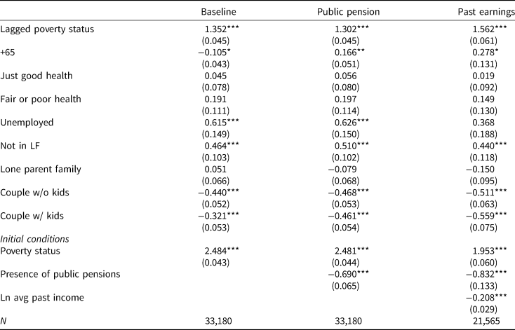
Note: For this exercise we use data for 2012–16 and we restrict the sample to individuals that are 50 or older. The dependent variable is an indicator function that takes the value one if the individual lives in a poor family (defined as having an income below 50% of the median income adjusted by census family size).
All these regressions control by education, house-hold composition, self-reported health and labour market status. The base category corresponds to a male head of the household who is 50–54 years old, who has no diploma, is living alone, reports having an excellent or very good health, is employed and not poor in the previous period. Is also not receiving a public pension at the beginning of the period. ***Significant at less than 1%; **significant at 5%; *significant at 10%.
The lower probability of poverty of those over 65 (first column) is likely to be attributable to the fact that individuals over that age can receive public pensions, since the association of being over 65 turns positive once public pensions are included in the regression.
Regression results also allow computing expected transition probabilities and poverty persistence for different groups. The probability of entering poverty for an individual receiving public pensions in 2012 is estimated as follows:

where Φ stands for the standard normal cdf and Z contains X as well as unobserved heterogeneity. This estimate is an average across individuals in the sample, taking the distribution of characteristics into account. The parameter α is associated with the dummy variable indicating the presence of public pensions. Results are shown in Table 9. The probability of entering poverty is 1.9% for those receiving public pensions in 2012, whereas it is twice as high, at 4%, for those not receiving public pensions. Those who receive public pensions thus are less likely to enter poverty, as well as less likely to be poor. The estimated persistence of poverty then is

Results indicate that those receiving public pensions are less likely to remain poor (14%) than those not receiving public pensions (26%). The probability of exit is simply 1 − Prob(p it = 1|p i,t−1 = 1, Z).
In sum, these results on entry differ from those obtained with the static model and presented in Table 7. When in our regression we control for lagged poverty and unobserved heterogeneity, the presence of public pensions is important in reducing entry into poverty. This difference is not surprising, since in this exercise we have modelled jointly the transitions into and out of poverty. Even if the results are not directly comparable, this exercise illustrates the robustness of our main findings.
7. Conclusion
In this paper, we analysed determinants of poverty among the elderly, with a particular focus on the role of public pensions. We have documented that poverty rates are lower for individuals who are over 65 years old. However, poverty is also more persistent for this group. Exploiting information on past earnings and past poverty from the administrative component of the dataset, we have shown that poverty after retirement is linked to more frequent spells of poverty before retirement. Public pension receipt is associated with lower levels of poverty among senior citizens. This relationship is driven by public pension receipts by those with low past earnings. This association persists even when controlling for past income history, as well as in a dynamic random effects probit model that controls for unobserved heterogeneity.
When looking at the dynamics of poverty, the probability of exit peaks at 65. Afterwards, the probability of exit is stable. The probability of entry decreases in age, up to age 65. Past this age, it increases slightly. Lower rates of poverty among older individuals reflect their comparatively low entry rate. Public pension receipt is associated with higher exit rates from poverty. Lower average past earnings and earlier years spent in poverty increase poverty both via higher entry and lower exit rates.
In conclusion, public pensions matter in alleviating poverty among the elderly but public pensions are far from eliminating poverty among seniors given that after controlling for unobserved heterogeneity, past poverty explains an important part of poverty at older ages. Individuals with low past average earnings during their careers have a higher probability of being poor when they are over 65 years old. This is important in a context where the indexation of the OAS to the consumer price index implies decreasing relative incomes of retirees, where population ageing increases the cost of public pensions, and where a higher age of pension eligibility is being considered. At the same time, changes in labour markets, in particular automation, could imply lower average earnings and a higher risk of poverty at older ages for some population groups. Basic public pension programmes could help those individuals, even if public pension benefits do not fully eradicate poverty at older ages. Moreover, more effort should be exerted in improving labour markets throughout each individual's working life and labour market inclusion.
Acknowledgements
We thank David Boisclair and Pierre-Carl Michaud for helpful comments. We also thank Simon Lord for his excellent research assistance. This research is also part of the programme of the Research Chair in Intergenerational Economics. Errors are our own. Some analyses reported in this paper were conducted at the Quebec Interuniversity Centre for Social Statistics (QICSS), which is part of the CRDCN. The services and activities provided by the QICSS are made possible by the financial or in-kind support of the SSHRC, CIHR, the CFI, Statistics Canada, FRQSC and the Quebec universities. The views expressed in this paper are those of the authors, and not necessarily those of the CRDCN or its partners.
Appendix A
Canada's pension system works on a PAYGO model with partially funded public pensions for workers. The first pillar is composed of the OAS; the GIS and the Allowance. The second pillar is the CQPP. It is partially funded by payroll taxes paid by both employees and employers, entirely portable and not tied to particular occupations or industries. There is also a third pillar that includes private pensions schemes that we do not describe in this paper.
The OAS provides a taxable uniform monthly grant to anyone aged 65 and over with some residency criteria. The payment (of $586.66 in Q1 of 2018) is reduced by 15 cents for each dollar of income, including CQPP income, in excess of a threshold of $74,788 in 2018.
This means that everyone except for individuals with high levels of income can receive this benefit.
The GIS is a non-taxable monthly grant to individuals aged 65 and over. It depends on household composition. The amount of the grant is a decreasing function of the level of family income. For example, in 2018 the maximum was $876.23 for singles, and $527.48 for each member of a couple. This grant is also income tested. For each dollar of family income (excluding the OAS), it is reduced by 50 cents for singles, and by 25 cents for each member of a couple.
Finally, the Allowance is paid to 60–64 year old spouses of GIS recipients and to 60–64 years old widows and widowers. It equals the OAS plus a fraction of the GIS for married individuals.
A proxy for the old-age safety net for a single person receiving the maximum amount of the OAS pension could be obtained by dividing the sum of the OAS pension (at age 65) and the GIS by the CQPP year's maximum pensionable earnings (YMPE, an approximate measure of average earnings). This old-age safety net for someone receiving the maximum amounts of OAS and GIS, which means they have worked very little (implying they have no CQPP income) in 2014 is approximately 30%.Footnote 35
The CQPP (the QPP for Quebec residents and the CPP for individuals in the Rest of Canada) benefits are entirely portable and not tied to particular occupations or industries.
The CQPP is partially funded by payroll taxes on employees and employers, and benefits are taxable. Benefits depend on an individual's earnings history via the following formula:


The earnings rating is the average of the ratio of an individual's annual earnings to the YMPE over the individual's earnings history, excluding the 15% of years with the lowest earnings, years caring for a child under 7 and years when disabled. The average is taken over earnings between the ages of 18 and of benefit claiming (between ages 60 and 70). For any year entering this average, the ratio is capped at 1. The pension adjustment factor is the average YMPE in the 5 years before retirement, including the year of retirement. The actuarial adjustment adjusts for age of retirement. The lowest age at which benefits can be received is 60. The adjustment reduces benefits by 0.5% for every month of retirement before the age of 65. Retiring later than at age 65 results in an increase of benefits by 0.5% per month. Finally, 0.25 is the replacement rate of the pension system, and the division by 12 results in the monthly benefit. Payments for all four components (OAS, GIS, Allowance) are adjusted quarterly for inflation and annually for the CQPP.
Appendix B
How the different measures of poverty have been computed
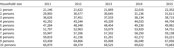
Low-income measures (LIMs): For international comparisons, the LIM is the most commonly used measure. The use of the LIM was suggested in 1989 in a paper by Wolfson, Evans, and the Organisation for Economic Co-operation and Development (OECD) which discussed their concerns about the LICOs. The LIM is a fixed percentage (50%) of median adjusted household income. Adjustment for household sizes reflects the fact that a household's needs increase as the number of members increases, although not necessarily proportionally.
The LIMs provided by Statistics Canada are calculated three times: with market income, before-tax income and after-tax and transfer income using the SLID. They do not require updating using an inflation index because they are calculated using an annual survey of household income. Unlike the LICOs, which are derived from an expenditure survey and then compared to an income survey, the LIMs are both derived and applied using a single income survey.
To calculate the LIMs, we first calculate the ‘equivalent household income’ for each household by dividing household income by its ‘adjusted size’, that is the square root of the number of persons in the household. Next, we assign this adjusted household income to each individual in the population. We then determine the median of this ‘equivalent household income’ over the population of individuals, that is the amount where half of all individuals will be above it and half below. The LIM for a household of one person is 50% of this median ‘equivalent household income’, and the LIMs for other sizes of households are equal to this value multiplied by their ‘equivalent household size’.
As explained earlier, the LIM used in Statistics Canada is calculated based on the household size and not the family. The logic behind it is that costs are usually shared within the household, even if you live with people outside of your family.
Table A.1. LIMs by income source and household size in current dollars
The LIM reported in our data is the LIM using census family. The reason is that this is the only measure available (or computable) in the administrative data.
Low-income cut-offs (LICOs): The LICOs are income thresholds below which a family will likely devote a larger share of its income on the necessities of food, shelter and clothing than the average family. The approach consists of estimating an income threshold at which families are expected to spend 20 percentage points more than the average family on food, shelter and clothing. The first set of published LICOs used the 1959 Family Expenditure Survey to estimate five different cut-offs varying between families of size one to five. These thresholds were then compared to family income from Statistics Canada's major income survey, the SCF, to produce low-income rates. Today, Statistics Canada continues to use this approach to construct LICOs, with the exception that cut-offs now vary by seven family sizes and five different populations of the area of residence. This additional variability is intended to capture differences in the cost of living among community sizes.
In order to account for changing spending patterns, Statistics Canada has in the past recalculated new LICOs after each subsequent Family Expenditure Survey.
After having calculated LICOs in the base year, cut-offs for other years are obtained by applying the corresponding consumer price index (CPI) inflation rate to the cut-offs from the base year – the process of indexing the LICOs. For example, continuing with the 1992 after-tax LICO for a family of four living in a community with a population between 30,000 and 99,999; to calculate the corresponding LICO for 2011, the CPI is used as follows:

The choice of after-tax income, total income or market income depends on whether one wants to take into account the added spending power that a family gets from receiving government transfers or its reduced spending power after paying taxes.
Statistics Canada produces two sets of LICOs and their corresponding rates – those based on total income (i.e., income including government transfers, before the deduction of income taxes) and those based on after-tax income. Derivation of before-tax versus after-tax LICOs is each done independently. There is no simple relationship, such as the average amount of taxes payable, to distinguish the two types of cut-offs.
Although both sets of LICOs and rates continue to be available, Statistics Canada prefers the use of the after-tax measure.
The choice to highlight after-tax rates was made for two main reasons. First, the before-tax rates only partly reflect the entire redistributive impact of Canada's tax/transfer system because they include the effect of transfers but not the effect of income taxes. Second, since the purchase of necessities is made with after-tax dollars, it is logical to use people's after-tax income to draw conclusions about their overall economic well-being.
Market basket measure (MBM): Canada's official measure of income poverty is the MBM from 2019. The MBM is based on the cost of a specific basket of goods and services representing a modest, basic standard of living. The basket is not fixed through time and is updated every few years. It includes the costs of food, clothing, footwear, transportation, shelter and other expenses for a reference family of two adults aged 25–49 and two children (aged 9 and 13). It provides thresholds for a finer geographic level than the LICO, allowing, for example, different costs for rural areas in the different provinces. These thresholds are compared to disposable income of families to determine low-income status. Disposable income is defined as the sum remaining after deducting the following from total family income: total income taxes paid; the personal portion of payroll taxes; other mandatory payroll deductions such as contributions to employer-sponsored pension plans, supplementary health plans and union dues; child support and alimony payments made to another family; out-of-pocket spending on child care and non-insured but medically prescribed health-related expenses such as dental and vision care, prescription drugs and aids for persons with disabilities.
The MBM thresholds are calculated as the cost of purchasing the following items: a nutritious diet as specified in the 2008 National Nutritious Food Basket; a basket of clothing and footwear required by a family of two adults and two children; shelter cost as the median cost of a two- or three-bedroom units including electricity, heat, water and appliances; transportation costs, using public transit where available or costs associated with owning and operating a modest vehicle where public transit is not available; and other necessary goods and services.
Appendix C
Table C.1. Distribution of years spent in poverty for different age groups for those who were poor at least once (as % of row and % of column)
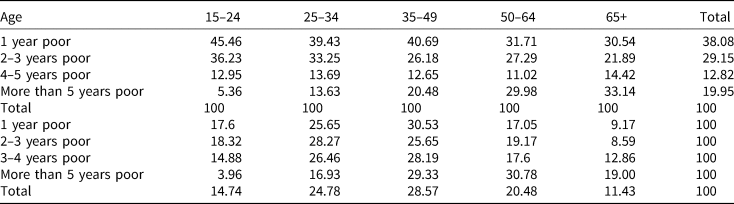
Table C.2. Longest spell length (for those who have been poor at least 1 year)
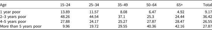
Table C.3. Role of public pensions and CQPP on the probability of being poor controlling for persistence and past average earnings
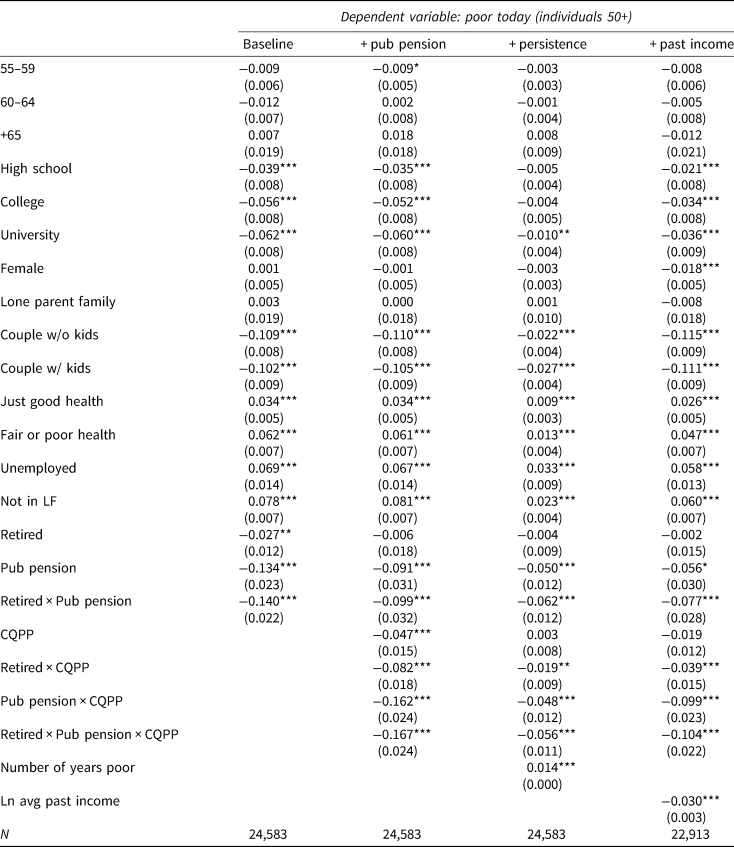
Table C.4. Poverty dynamics – probability of exiting poverty with public pensions and CQPP (restricting the sample to individuals 50 and older)
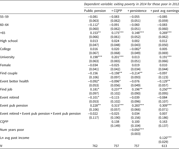
Table C.5. Poverty dynamics – probability of entering poverty with public pensions and CQPP (restricting the sample to individuals 50 and older)
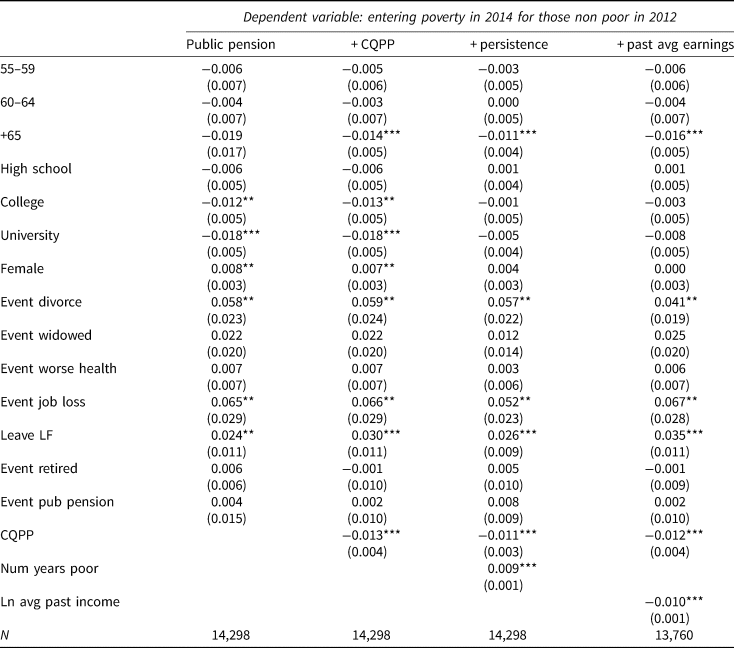
Table C.6. Probability of being poor conditional on demographic characteristics using LICO and MBM (Individuals +50)


 Open access