


Nomenclature
- UAV
unmanned aerial vehicle
- VTOL
vertical takeoff and landing
- TRUAV
tiltrotor unmanned aerial vehicle
- CSF-TRUAV
control surface free tiltrotor unmanned aerial vehicle
- CFD
computational fluid dynamics
- ESO
extended state observer
- LQR
linear quadratic regulator
- MRAC
model reference adaptive control
- MPC
model predictive controller
- DOF
degree of freedom
- PID
proportional integral derivative
Greek Symbol
- $\phi ,\theta ,\psi $
-
roll, pitch and heading angle
-
$\gamma $
-
tilt angle
-
$\alpha ,\beta $
-
angle-of-attack and side slip angle
-
${\rm{\Omega }}$
-
angular velocity
-
$\rho $
-
air density


1.0 Introduction
Unmanned aerial vehicles (UAVs) have attracted considerable attention during the last couple of decades, because of the wide range of applications they can be employed in. These include security and surveillance [Reference Miller, Stepanyan, Popov and Miller1–Reference Ayar, Dalkiran, Kale, Nagy and Karakoc3], real-time monitoring of natural disasters [Reference Cui, Phang, Ang, Wang, Dong, Ke, Lai, Li, Li, Lin, Liu, Pang, Wang, Yang, Lin and Chen4], inspection of strategic infrastructures [Reference Lei, Wang, Xu and Song5, Reference Bouras, Bouzid and Guiatni6], aerial manipulation [Reference Shirani, Najafi and Izadi7–Reference Zhao, Luo, Wang and Shen9], logistics and delivery services [Reference Guan, Li and Zeng10], to name but a few.
According to their lift generation principle, UAVs have classically been categorised into two main categories: fixed-wing drones, which use wings and fuselage to generate lift, and rotary-wing drones, where the lift is produced by the rotors. Rotary-wing drones have the advantages of ease of use, high manoeuvrability, and vertical takeoff and landing capabilities, but suffer from limited endurance. On the other hand, fixed-wing drones have long endurance and a high cruising speed. However, they lack manoeuvrability and cannot land or take off vertically, nor perform a stationary flight.
The limited autonomy of rotary-wing drones and the incapacity of their fixed-wing counterpart to perform stationary flights make them both unsuitable for several applications. Among these one can mention: delivery to distant places, close surveillance of remote areas and the tracking of a faraway target moving at variable speed profiles.
The above mentioned limitations have motivated drone experts to consider new designs that combine the features of fixed and rotary-wing drones. These designs fall into the category of convertible or hybrid drones. Such solutions target the high cruising speed and autonomy of fixed-wing drones and the stationary flight capacity of rotary-wing drones. Their vertical takeoff and landing capability further allow resolving the issue of the requirement for a runway and a large open space, and also reduces maintenance costs due to the smooth vertical landing.
Convertible drones can be broadly categorised into two main classes [Reference Saeed, Younes, Cai and Cai11]. The first encompasses tail-sitters, which take off and land on their tails. As illustrated in Fig. 1, these drones tilt their entire fuselage to transit from stationary to cruise flight and vice versa. The principal drawback of tail-sitters is that they operate at a high angle-of-attack, making them very sensitive to crosswinds, particularly while in hover mode.
The transition in tail-sitter drones is controlled using both control surfaces and rotor tilting. Several techniques have been proposed in the literature. Stone [Reference Stone12] used the “stall-tumble” technique for forward transition and pull-up to vertical manoeuvre for back transition. In Refs. [Reference Stone and Clarke13, Reference Li, Sun, Zhou, Wen, Low and Chen14] unstalled vertical-to-horizontal transition was applied using optimisation to minimise the transition time. Boyan et al. [Reference Li, Sun, Zhou, Wen, Low and Chen14] applied a continuous ascending trajectory by gradually increasing the altitude while transitioning from nearly vertical to horizontal flight.
In the second category, commonly named ‘convertiplanes’, the drone maintains the same orientation of its main fuselage in all flight phases. The transition is commonly achieved by tilting the wings or rotors using the thrust vectoring concept [Reference Allenspach and Ducard15, Reference Yu, Zhang and Wang16]. The category of convertiplanes can be further divided into three subcategories as depicted in Fig. 2. The first is tilt-wings, such as the ‘DHL Parcelcopter V3.0’ used for delivery services, Fig. 2(a). These drones tilt their entire wings to transition between flight modes, which makes them very sensitive to crosswind. The second category is that of dual systems, which use a set of rotors for hovering and other pusher rotors for cruise flight. This simplifies the control of the at the cost of the increased weight and price. An example of this category is the ‘Wingcopter 198’ illustrated in Fig. 2(b). The last subcategory of convertiplanes is that of tilt-rotors, such as the “Turac” [Reference Yuksek, Vuruskan, Ozdemir, Yukselen and Inalhan17] UAV, depicted in Fig. 2(c).
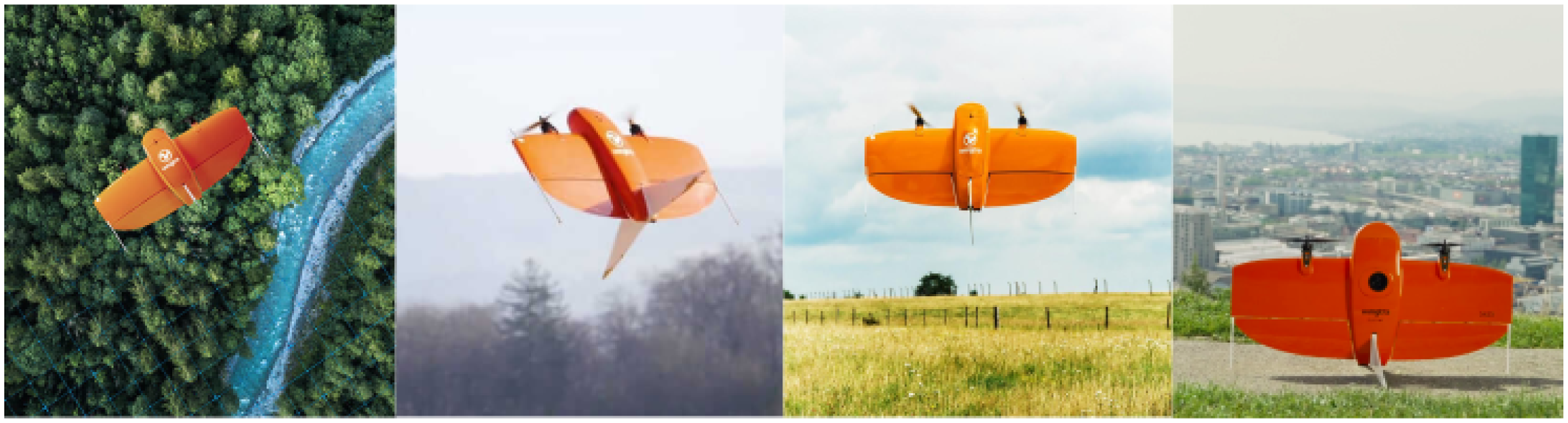
Figure 1. WingtraOne tailsitter with different flight modes: hover, transition and cruise.
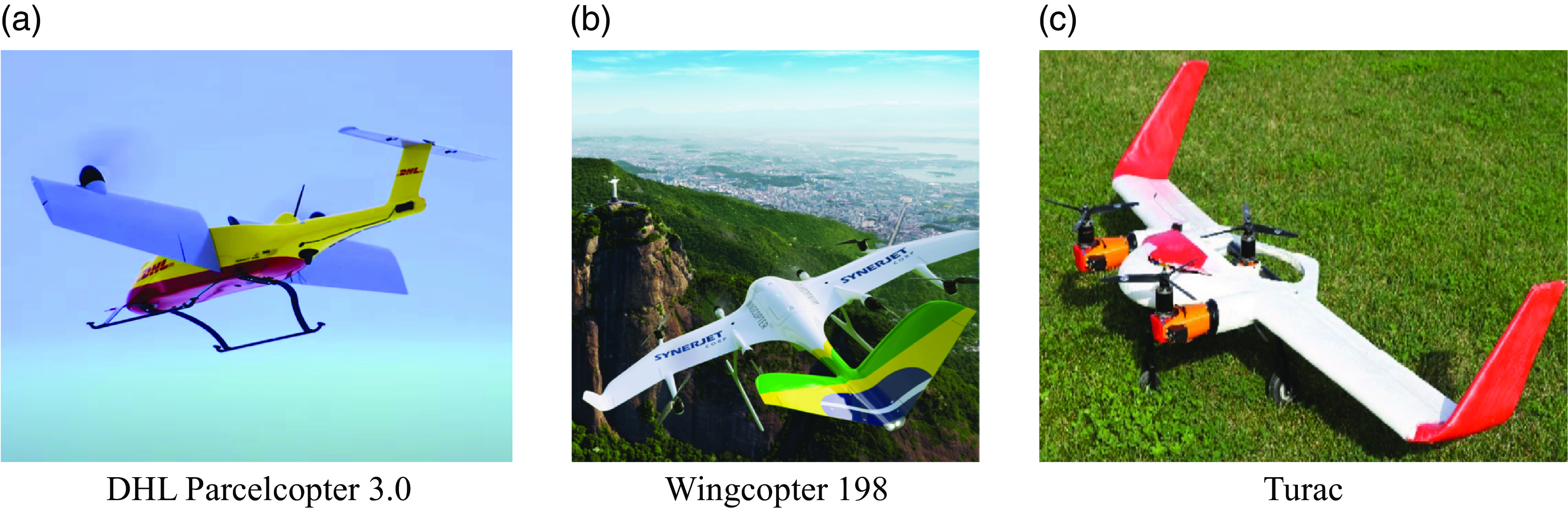
Figure 2. Examples of convertiplane drones.
Due to their simple transition mechanism, operation at a low angle-of-attack and enhanced vertical flight stability compared to tilt-wings and tail-sitters, TRUAVs present a good trade-off in terms of aerodynamic performances and controllability [Reference Saeed, Younes, Cai and Cai11]. On the other hand, the aerodynamic consequences of changing force directions and speed profiles, and the resulting dynamic model variation make controlling TRUAVs a challenging task.
A TRUAV can be termed dual or multi according to its number of rotors. Dual-TRUAVs use two rotors, generally placed on the wingtip [Reference Liu, He, Yang and Han18]. This design increases the complexity, especially at low airspeeds, where the effect of the downwash generated by the rotors on the wings becomes important [Reference Appleton, Filippone and Bojdo19]. Multi-TRUAVs have more than two rotors, three (3) or four (4) rotors in most cases. This subcategory is characterised by a simpler mechanical design and a reduced rotor effect on the wings compared to Dual-TRUAVs [Reference Yeo and Johnson20].
The drone considered in this work falls into the category of multi-TRUAVs. It is composed of four rotors placed symmetrically with respect to the drone’s centre of mass. This design differs from that adopted in previous works, where the rotors are only employed for generating thrust forces: the lift force when in hover mode and the pushing force when in fixed-wing mode. In addition to the rotors, control surfaces are used for controlling the drone’s attitude while in fixed-wing configuration.
In this work, a clean configuration design is considered, i.e., which does not include any control surfaces. The rotors of the drone are responsible for generating the necessary thrust forces as well as controlling the attitude of the drone–not only in VTOL mode but also when in cruise flight. This configuration allows minimising the interference induced by the rotors’ downwash with non-retracted control surfaces as well as the drag created by these surfaces. Furthermore, the proposed design avoids one of the reasons for the complexity of TRUAVs control, which is the inefficiency of control surfaces during the transition phase.
In terms of control, and to the authors’ knowledge, all previous works consider two controllers for each flight mode and implement a switching strategy to ensure a successful transition. A new control scheme, which employs a single controller for both flight modes, is proposed in this work. The proposed solution allows the UAV to fly at both low and high speeds. This is particularly important for applications requiring to make stops along the route, such as convoy surveillance and the tracking of moving ground targets.
In terms of energetic performances, the proposed design and associated control strategy lie between multirotor and fixed-wing drones. In fact, when the drone enters cruise mode, less demand is put on the rotors leading to a reduction in power consumption compared to a multirotor. This is, however, less efficient compared to fixed-wing drones, because of the usage of rotors for controlling the attitude instead of the control surfaces. Since these surfaces are actuated using servomotors, they consume less power compared to the rotors, commonly actuated using BLDC motors.
The contributions of this work can be summarised in the following
-
A detailed model for a control surface free tilt-rotor UAV (CSF-TRUAV), based on the parametres of the famous Zagi flying wing.
-
A new control strategy that employs a single controller to handle both VTOL and fixed-wing modes. The proposed strategy further allows controlling the pitch angle independently from the forward motion.
-
Design, validation and robustification of a nonlinear controller for trajectory tracking based on a backstepping approach.
The research methodology followed in this paper is summarised in Fig. 3. The Kinematic and dynamic model for the CSF-TRUAV is derived in Section 3. The parametres of this model are those of the famous Zagi flying wing drone. The obtained model features high non-linearities and coupling, which require making some simplifications for the control design. Section 4 discusses the proposed control scheme and the design of nonlinear controllers. The designed controllers are validated on the full non-linear model, i.e. the model without simplifications. The validation scenario and obtained results are presented in Section 5. To provide the context of the present work, a literature review related to the TRUAV category is carried out in the next section.
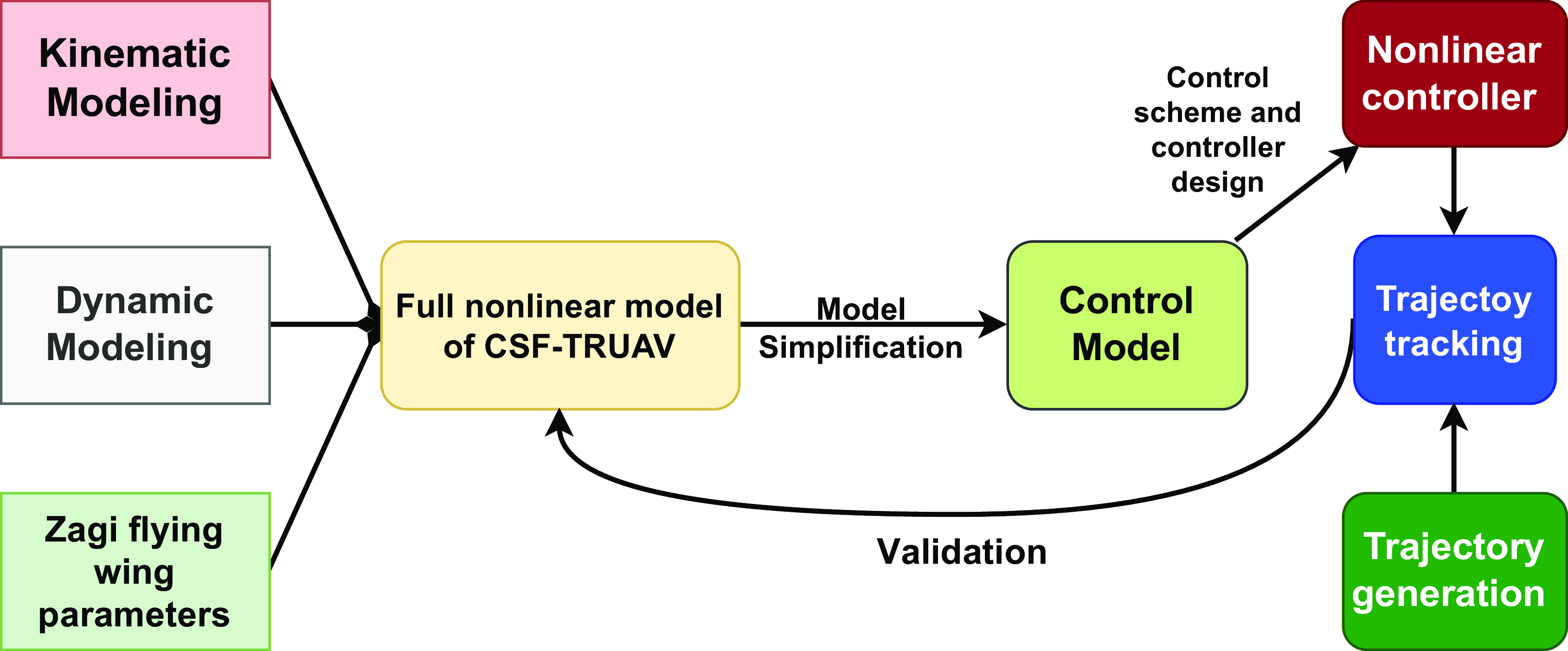
Figure 3. Summary of the research methodology followed in this paper.
2.0 Related works
Given the large number of research works related to convertible UAVs, this section will only focus on those works that have dealt with the tilt-rotor category. For more details about other works the reader is referred to the surveys in Refs. [Reference Saeed, Younes, Cai and Cai11, Reference Ducard and Allenspach21], which present a rigorous categorisation of convertible UAV designs, their technical characteristics, and existing control strategies.
It is worth noting that the term “TRUAV” discussed in this work is not to be confused with tilt-multirotors, such as the tilt-quadrotor in Refs. [Reference Papachristos, Alexis and Tzes22, Reference Kumar, Kumar, Cohen and Cazaurang23] and tilt-trirotor in Ref. [Reference Papachristos, Alexis and Tzes24]. These are simply extensions of multirotors [Reference Derrouaoui, Bouzid and Guiatni25], targeting to add more degrees of freedom and hence deal with complex trajectory tracking, enhance stability and make the drone fully actuated, which is another topic.
Among the works which have dealt with the modeling of TRUAVs, Yuksek et al. [Reference Yuksek, Vuruskan, Ozdemir, Yukselen and Inalhan17] presented detailed dynamic and aerodynamic models with advanced calculations of fluid dynamics (CFD). They also performed experimental tests in a wind tunnel to analyse the aerodynamic behaviour of the rotors and wings under different flight conditions. Nevertheless, they disregarded the design of the controller, which is an essential part to ensure stability.
Since TRUAVs are characterised by a strongly nonlinear model, the application of linear control solutions for such systems is not straightforward. Chen et al. [Reference Chen and Jia26] linearised the dynamic equations around the hovering conditions and proposed a trim-based control allocation approach. A robust servo linear quadratic regulator (RSLQR) was considered for the control design, combined with an extended state observer (ESO) to reconstruct the non-measurable states of the drone.
Similarly, a flight controller for the six degrees of freedom of a TRUAV was developed by Hegde et al. [Reference Hegde, George, Nayak and Kumar27] using an H-infinity optimisation with loop shaping. The designed controller, however, was only validated for the pitch and attack angles using two control inputs, the elevator and aileron deflections.
Ta et al. [Reference Ta, Fantoni and Lozano28] combined a linear proportional integral derivative (PID) controller with a nonlinear saturated sigmoid function to stabilise the pitch angle of a three-rotor TRUAV. For the position, the authors used an adaptive controller based on a neural network. The proposed controller does not, however, take into account the cross-coupling between the states, which may affect its efficiency during the transition phase.
The performance of linear controllers gradually degrades as the vehicle states deviate from the equilibrium point. This is a fundamental concern for the class of convertible UAVs that operate far from the equilibrium point during the transition phase [Reference Hegde, George, Nayak and Kumar27]. Flores et al. [Reference Flores, Escareño, Lozano and Salazar29] used a nonlinear backstepping controller for cruise flight. In hover mode, the TRUAV was controlled using a feedback linearisation solution as if it was a conventional multirotor.
In another work, Flores et al. [Reference Flores and Lozano30] proposed a control technique for the transition manoeuvre. The desired altitude was maintained during the transition phase, using a nested saturation control approach. The control input vector was composed of the tilt angle, total rotors thrust, the difference of thrust between the front and rear rotors, and the elevator deflection.
Tavoosi et al. [Reference Tavoosi31] used a model reference adaptive control (MRAC) for the vertical flight phase, and a model predictive controller (MPC) when the drone switches to horizontal flight. A perceptron neural network was used to compensate for the discrepancy between the linearised model and the real nonlinear model of the drone.
In order to meet trajectory tracking requirements and enhance the forward flight of a tilt-rotor UAV, the authors in Ref. [Reference Cardoso, Esteban and Raffo32] used a robust adaptive mixing controller to handle actuator redundancy in horizontal and transition modes.
Su et al. [Reference Su, Qu, Zhu, Swei, Hashimoto and Zeng33] derived the nonlinear dynamic equations of a tiltrotor UAV. The model was then linearised around the trimming conditions to generate linear time-invariant state-space models. Adaptive model predictive control (MPC) was used as the controller for each linear model. Di Francesco et al. [Reference Francesco and Mattei34] adopted a component build-up approach to model the nonlinear dynamics of a tilt-rotor UAV. To address challenges related to nonlinearities, and cross-coupling effects, the authors employed an incremental nonlinear dynamic inversion technique for the design of the flight controller.
Hou et al. [Reference Hou, Cai, Liu, Zhao, Wang and Wu35] implemented a gain scheduling solution to deal with the transition phase of a quad TRUAV. The altitude of the drone was controlled using the elevator and the four throttles, with gains depending on the tilt angle. Hernandez-Garcia et al. [Reference Hernandez-Garcia and Rodriguez-Cortes36] applied a gain scheduling controller for a dual TRUAV. A set of controllers was designed based on Jacobian linearization of the drone’s model around: takeoff, vertical, hovering, and horizontal flight conditions.
The main drawback of gain scheduling techniques is that the performance is only guaranteed at the design points, and additional stability and performance analysis must be derived through extensive simulation and testing [Reference Bett and Chen37]. Typically, successful designs involve scheduling on a slowly changing variable. This is not the case for applications requiring high maneuverability of the drone such as the tracking of ground targets.
The work in Ref. [Reference Kong and Lu38] is, to the authors’ view, the closest to the present work in terms of structural design. Regarding the control, however, the authors in Ref. [Reference Kong and Lu38] used two separate controllers for each flight phase, which brings about the disadvantages discussed previously. Furthermore, the rotor model adopted was too simplistic, since it neglected the drag torque. The aerodynamic model was also too simplistic, as it considered the lift and drag forces independent of the angle-of-attack, side-slip angle, and angular rates.
The novelty of the present work, in addition to the derivation of a more realistic model, is to use just the rotors as control input and to not involve control surfaces. Such a solution not only simplifies the design of the drone but also ensures a safe transition between hover and cruise flight and vice-versa. This is made possible thanks to a novel control scheme which employs a single controller to handle both VTOL and fixed-wing modes.
The proposed control strategy is validated on the full nonlinear model of the drone, including all the couplings and actuators saturation. This strategy can also be used with classical designs that include control surfaces, as a redundant solution for fault tolerance.
3.0 Modeling of the CSF-TRUAV
The control-surface-free TRUAV considered in this work is illustrated in Figs. 4 and 5. It is actuated by four rotors symmetrically placed on both sides of the wings. The 3D positions, ${P_i}$
, of each rotor are denoted.
${P_i}$
, of each rotor are denoted.
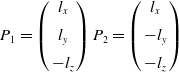 \begin{align}{P_1} = \left( {\begin{array}{c}{{l_x}}\\[5pt] {{l_y}}\\[5pt] { - {l_z}}\end{array}} \right){P_2} = \left( {\begin{array}{c}{{l_x}}\\[5pt] { - {l_y}}\\[5pt] { - {l_z}}\end{array}} \right)\end{align}
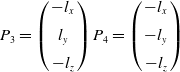 \begin{align}{P_3} = \left( {\begin{array}{c}{ - {l_x}}\\[5pt] {{l_y}}\\[5pt] { - {l_z}}\end{array}} \right){P_4} = \left( {\begin{array}{c}{ - {l_x}}\\[5pt] { - {l_y}}\\[5pt] { - {l_z}}\end{array}} \right)\end{align}
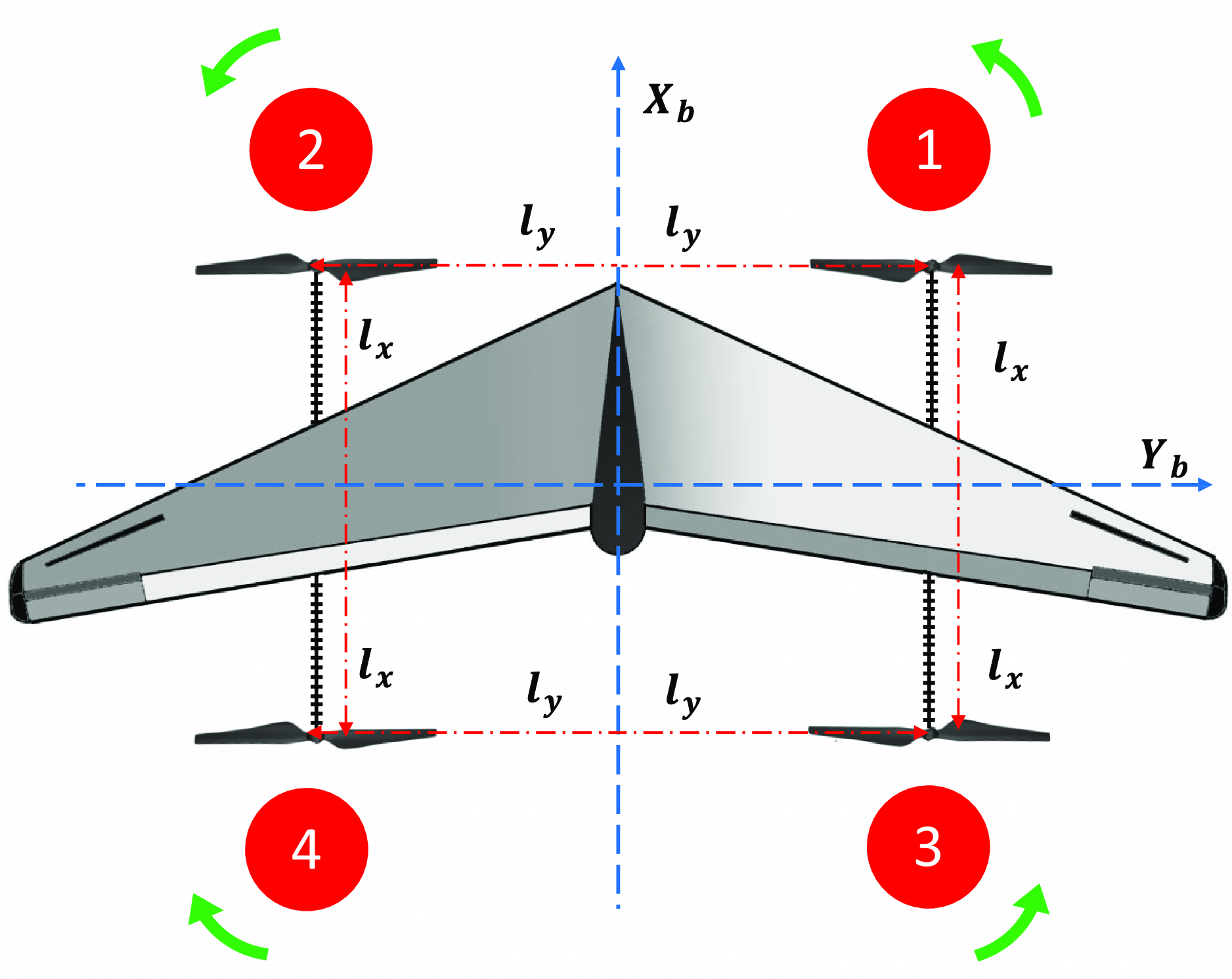
Figure 4. CSF-TRUAV model top view illustration.
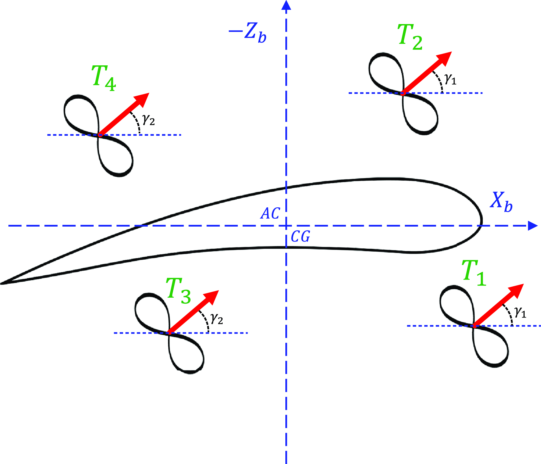
Figure 5. CSF-TRUAV model side view illustration.
This design seems at first glance similar to those in Refs. [Reference Chen and Jia26, Reference Flores, Escareño, Lozano and Salazar29]. Nevertheless, both of these works consider control surfaces, which is not the case in the present work.
After developing and analysing the inverse dynamic model of a CSF-TRUAV with four independently tiltable rotors, it was concluded that this design is over-actuated. To further simplify the mechanical structure, two constraints are considered. The first is that the front rotors tilt with the same angle, denoted ${\gamma _1}$
. The second constraint is to fix the tilt angle of the back rotors to a fixed angle
${\gamma _1}$
. The second constraint is to fix the tilt angle of the back rotors to a fixed angle ${\gamma _2} = \pi /2$
.
${\gamma _2} = \pi /2$
.
The resulting structure, which features only two front tilting rotors, is illustrated in Fig. 6. Given this configuration, the front rotors might be coupled using a single actuator, which offers a further simplification of the drone structure.
Figure 6. Structure of the control surface free tilt-rotor UAV.
The application of Newton’s second law gives the following equations for the dynamic model of the CSF-TRUAV
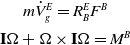 \begin{align}\begin{array}{c}{m{{\dot V}_g}^E = R_B^E{F^B}} {}\\[5pt] {{\bf{I}}{\rm{\Omega }} + {\rm{\Omega }} \times {\bf{I}}{\rm{\Omega }} = {M^B}} {}\end{array}\end{align}
where $E = \left( {\begin{array}{c}{{X_E},{Y_E},{Z_E}}\end{array}} \right)$
denotes the Earth centred inertial frame, and
$E = \left( {\begin{array}{c}{{X_E},{Y_E},{Z_E}}\end{array}} \right)$
denotes the Earth centred inertial frame, and $B = \left( {\begin{array}{c}{{X_B},{Y_B},{Z_B}} \end{array}} \right)$
refers to the body-fixed frame. The transition matrix from the body frame to the inertial frame,
$B = \left( {\begin{array}{c}{{X_B},{Y_B},{Z_B}} \end{array}} \right)$
refers to the body-fixed frame. The transition matrix from the body frame to the inertial frame, $R_B^E$
, is given by
$R_B^E$
, is given by
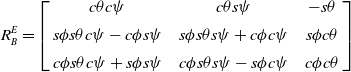 \begin{align}R_B^E = \left[ {\begin{array}{c@{\quad}c@{\quad}c}{c\theta c\psi } & {c\theta s\psi } & { - s\theta }\\[5pt] {s\phi s\theta c\psi - c\phi s\psi } & {s\phi s\theta s\psi + c\phi c\psi } & {s\phi c\theta }\\[5pt] {c\phi s\theta c\psi + s\phi s\psi }& {c\phi s\theta s\psi - s\phi c\psi } & {c\phi c\theta }\end{array}} \right]\end{align}
with $sa = {\rm{sin}}\!\left( a \right)$
,
$sa = {\rm{sin}}\!\left( a \right)$
, $ca = {\rm{cos}}\!\left( a \right)$
, and
$ca = {\rm{cos}}\!\left( a \right)$
, and $\varphi $
,
$\varphi $
, $\theta $
and
$\theta $
and $\psi $
the roll, pitch and yaw angles, respectively. The kinematics of the drone are given by the equations
$\psi $
the roll, pitch and yaw angles, respectively. The kinematics of the drone are given by the equations
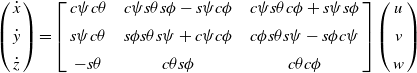 \begin{align}\left( {\begin{array}{c}{\dot x}\\[5pt] {\dot y}\\[5pt] {\dot z}\end{array}} \right) = \left[ {\begin{array}{c@{\quad}c@{\quad}c}{c\psi c\theta } & {c\psi s\theta s\phi - s\psi c\phi } & {c\psi s\theta c\phi + s\psi s\phi }\\[5pt] {s\psi c\theta } & {s\phi s\theta s\psi + c\psi c\phi } & {c\phi s\theta s\psi - s\phi c\psi }\\[5pt] { - s\theta } & {c\theta s\phi } & {c\theta c\phi }\end{array}} \right]\left( {\begin{array}{c}u\\[5pt] v\\[5pt] w\end{array}} \right)\end{align}
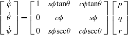 \begin{align}\left[ {\begin{array}{c}{\dot \varphi }\\[5pt] {\dot \theta }\\[5pt] {\dot \psi }\end{array}} \right] = \left[ {\begin{array}{c@{\quad}c@{\quad}c}1& {s\phi {\rm{tan}}\theta } & {c\phi {\rm{tan}}\theta }\\[5pt] 0 & {c\phi } & { - s\phi }\\[5pt] 0 & {s\phi {\rm{sec}}\theta } & {c\phi {\rm{sec}}\theta }\end{array}} \right]\left[ {\begin{array}{c}p\\[5pt] q\\[5pt] r\end{array}} \right]\end{align}
with $u$
,
$u$
, $v$
and
$v$
and $w$
denote the linear velocity, while
$w$
denote the linear velocity, while $p$
,
$p$
, $q$
, and
$q$
, and $r$
represent the angular rates, both expressed in the body frame. Variables
$r$
represent the angular rates, both expressed in the body frame. Variables $x$
,
$x$
, $y$
and
$y$
and $z$
refer to the drone position with respect to the inertial frame.
$z$
refer to the drone position with respect to the inertial frame.
According to the blade elements and momentum theory [Reference Adkins and Liebeck39], the thrust forces, ${T_i}$
, and moments,
${T_i}$
, and moments, ${C_i}$
, generated by each rotor can be approximated as proportional to the square of the rotor’s rotating speed
${C_i}$
, generated by each rotor can be approximated as proportional to the square of the rotor’s rotating speed ${\omega _i}$
 \begin{align}\left\{ {\begin{array}{c}{{T_i} = {K_l}\omega _i^2}\\[5pt] {{C_i} = {K_c}\omega _i^2}\end{array}} \right.\end{align}
with ${K_l}$
and
${K_l}$
and ${K_c}$
the thrust and drag coefficients. These variables depend on the air density, the chord of the blade surface, the aerodynamic coefficients of the wing profile, the number of blades and the angle-of-attack. Let
${K_c}$
the thrust and drag coefficients. These variables depend on the air density, the chord of the blade surface, the aerodynamic coefficients of the wing profile, the number of blades and the angle-of-attack. Let ${K_{ld}} = {K_c}/{K_l}$
denotes the constant of proportionality between the two coefficients, this gives
${K_{ld}} = {K_c}/{K_l}$
denotes the constant of proportionality between the two coefficients, this gives
 \begin{align}{C_i} = {K_{ld}}{T_i}\end{align}
The drag torque and thrust force expressed in the frame ${R_i}$
linked to the rotor
${R_i}$
linked to the rotor $i$
are given by
$i$
are given by
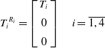 \begin{align}{T_i}^{{R_i}} = \left[ {\begin{array}{c}{{T_i}}\\[5pt] 0\\[5pt] 0\end{array}} \right]\quad i = \overline {1,4} \end{align}
The transition matrices from a rotor-linked frame to the body frame, denoted as $R_{1,2}^B$
for the front rotors and
$R_{1,2}^B$
for the front rotors and $R_{3,4}^B$
for rear rotors, are given by
$R_{3,4}^B$
for rear rotors, are given by
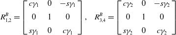 \begin{align}R_{1,2}^B = \left[ {\begin{array}{c@{\quad}c@{\quad}c}{c{\gamma _1}} & 0 & { - s{\gamma _1}}\\[5pt] 0 & 1 & 0\\[5pt] {s{\gamma _1}} & 0 & {c{\gamma _1}}\end{array}} \right],{\rm{\;\;\;\;}}R_{3,4}^B = \left[ {\begin{array}{c@{\quad}c@{\quad}c}{c{\gamma _2}} & 0 & { - s{\gamma _2}}\\[5pt] 0 & 1 & 0\\[5pt] {s{\gamma _2}} & 0 & {c{\gamma _2}}\end{array}} \right]\end{align}
The total thrust force generated by the four rotors can be written as
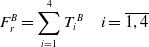 \begin{align} F_{r}^B=\sum_{i=1}^{4}T_{i}{ }^{B} \quad i=\overline{{1,4}} \end{align}
with $T_i^B$
the thrust force generated by each rotor expressed in the body frame,
$T_i^B$
the thrust force generated by each rotor expressed in the body frame,
 \begin{align}T_i^B = R_{i,i + 1}^B{T_i}^{{R_i}}\end{align}
After development, the total thrust force simplifies to
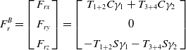 \begin{align}F_r^B = \left[ {\begin{array}{c}{{F_{rx}}}\\[5pt] {{F_{ry}}}\\[5pt] {{F_{rz}}}\end{array}} \right] = \left[ {\begin{array}{c}{{T_{1 + 2}}C{\gamma _1} + {T_{3 + 4}}C{\gamma _2}}\\[5pt] 0\\[5pt] { - {T_{1 + 2}}S{\gamma _1} - {T_{3 + 4}}S{\gamma _2}}\end{array}} \right]\end{align}
where ${T_{1 + 2}} = {T_1} + {T_2}$
and
${T_{1 + 2}} = {T_1} + {T_2}$
and ${T_{3 + 4}} = {T_3} + {T_4}$
.
${T_{3 + 4}} = {T_3} + {T_4}$
.
The drag torque generated by each rotor is expressed in the local frame as
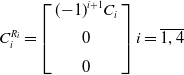 \begin{align}C_i^{{R_i}} = \left[ {\begin{array}{c}{{{(\!-\! 1)}^{i + 1}}{C_i}}\\[5pt] 0\\[5pt] 0\end{array}} \right]i = \overline {1,4} \end{align}
The torque generated by each rotor is a combination of the drag torque and the moment resulting from the thrust forces,
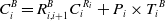 \begin{align}C_i^B = R_{i,i + 1}^B{C_i}^{{R_i}} + {P_i} \times {T_i}^B\end{align}
The total moment generated by the four rotors is expressed w.r.t. the body frame as
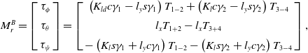 \begin{align}M_r^B = \left[ {\begin{array}{c}{{\tau _\phi }}\\[5pt] {{\tau _\theta }}\\[5pt] {{\tau _\psi }}\end{array}} \right] = \left[ {\begin{array}{c}{\left( {{K_{ld}}c{\gamma _1} - {l_y}s{\gamma _1}} \right){T_{1 - 2}} + \left( {{K_l}c{\gamma _2} - {l_y}s{\gamma _2}} \right){T_{3 - 4}}}\\[5pt] {{l_x}{T_{1 + 2}} - {l_x}{T_{3 + 4}}}\\[5pt] { - \left( {{K_l}s{\gamma _1} + {l_y}c{\gamma _1}} \right){T_{1 - 2}} - \left( {{K_l}s{\gamma _2} + {l_y}c{\gamma _2}} \right){T_{3 - 4}}}\end{array}} \right],\end{align}
with ${T_{1 - 2}} = {T_1} - {T_2}$
and
${T_{1 - 2}} = {T_1} - {T_2}$
and ${T_{3 - 4}} = {T_3} - {T_4}$
.
${T_{3 - 4}} = {T_3} - {T_4}$
.
Assuming a small angle-of-attack and that the airflow remains laminar and attached, the aerodynamic forces ${F_a} = \left[ {\begin{array}{c@{\quad}c@{\quad}c}L & D & {{f_y}}\end{array}} \right]$
and moments
${F_a} = \left[ {\begin{array}{c@{\quad}c@{\quad}c}L & D & {{f_y}}\end{array}} \right]$
and moments ${M_a} = \left[ {\begin{array}{c@{\quad}c@{\quad}c}{{l_a}} & {{m_a}} & {{n_a}}\end{array}} \right]$
expressed in the wind frame,
${M_a} = \left[ {\begin{array}{c@{\quad}c@{\quad}c}{{l_a}} & {{m_a}} & {{n_a}}\end{array}} \right]$
expressed in the wind frame, ${R_w}$
, can be approximated as [Reference Beard and McLain40]
${R_w}$
, can be approximated as [Reference Beard and McLain40]
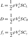 \begin{align}\begin{array}{c}L\; { = \dfrac{1}{2}\rho V_a^2S{C_L}} \\[12pt] D \;{ = \dfrac{1}{2}\rho V_a^2S{C_D}} \\[12pt] {{f_y}} \;{ = \dfrac{1}{2}\rho V_a^2S{C_y}} \end{array}\end{align}
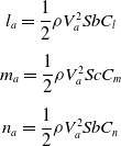 \begin{align}\begin{array}{c}{{l_a}}\; { = \dfrac{1}{2}\rho V_a^2Sb{C_l}} \\[12pt] {{m_a}}\; { = \dfrac{1}{2}\rho V_a^2Sc{C_m}} \\[12pt] {{n_a}}\; { = \dfrac{1}{2}\rho V_a^2Sb{C_n}} {}\end{array}\end{align}
with ${V_a}$
the resultant air mass velocity, calculated as the difference between the drone’s ground speed and the wind speed:
${V_a}$
the resultant air mass velocity, calculated as the difference between the drone’s ground speed and the wind speed: ${V_a} = {V_g} - {V_{wind}}$
.
${V_a} = {V_g} - {V_{wind}}$
. $S$
is the wing area;
$S$
is the wing area; $c$
is the mean chord; and
$c$
is the mean chord; and $b$
is the wing span. The aerodynamic coefficients reduce to the equations below [Reference Beard and McLain40]
$b$
is the wing span. The aerodynamic coefficients reduce to the equations below [Reference Beard and McLain40]
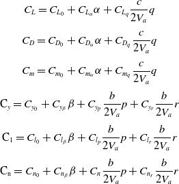 \begin{align}\begin{array}{c}{{C_L} = {C_{{L_0}}} + {C_{{L_\alpha }}}\alpha + {C_{{L_q}}}\dfrac{c}{{2{V_a}}}q}\\[12pt] {{C_D} = {C_{{D_0}}} + {C_{{D_\alpha }}}\alpha + {C_{{D_q}}}\dfrac{c}{{2{V_a}}}q}\\[12pt] {{C_m} = {C_{{m_0}}} + {C_{{m_\alpha }}}\alpha + {C_{{m_q}}}\dfrac{c}{{2{V_a}}}q}\\[12pt] {{{\rm{C}}_y} = {C_{{y_0}}} + {C_{{y_\beta }}}\beta + {C_{{y_p}}}\dfrac{b}{{2{V_a}}}p + {C_{{y_r}}}\dfrac{b}{{2{V_a}}}r}\\[12pt] {{{\rm{C}}_1} = {C_{{l_0}}} + {C_{{l_\beta }}}\beta + {C_{{l_p}}}\dfrac{b}{{2{V_a}}}p + {C_{{l_r}}}\dfrac{b}{{2{V_a}}}r}\\[12pt] {{{\rm{C}}_{\rm{n}}} = {C_{{n_0}}} + {C_{{n_\beta }}}\beta + {C_{{n_{}}}}\dfrac{b}{{2{V_a}}}p + {C_{{n_r}}}\dfrac{b}{{2{V_a}}}r}\end{array}\end{align}
with $\alpha $
the angle-of-attack, and
$\alpha $
the angle-of-attack, and $\beta $
the side slip angle.
$\beta $
the side slip angle.
The resulting aerodynamic force expressed w.r.t. the body frame, $F_a^B$
, is given by
$F_a^B$
, is given by
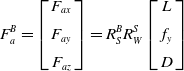 \begin{align}F_a^B = \left[ {\begin{array}{c}{{F_{ax}}}\\[5pt] {{F_{ay}}}\\[5pt] {{F_{az}}}\end{array}} \right] = R_S^BR_W^S\left[ {\begin{array}{c}L\\[5pt] {{f_y}}\\[5pt] D\end{array}} \right]\end{align}
with $R_W^S$
and
$R_W^S$
and $R_S^B$
the transition matrices from the wind to the stability frame and from the stability frame to the body frame, respectively
$R_S^B$
the transition matrices from the wind to the stability frame and from the stability frame to the body frame, respectively
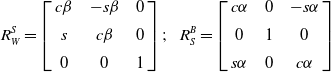 \begin{align}R_W^S = \left[ {\begin{array}{c@{\quad}c@{\quad}c}{c\beta } & { - s\beta }& 0\\[5pt] s & {c\beta }& 0\\[5pt] 0& 0& 1\end{array}} \right];{\rm{\;\;\;\;}}R_S^B = \left[ {\begin{array}{c@{\quad}c@{\quad}c}{c\alpha }& 0 &{ - s\alpha }\\[5pt] 0 &1 &0\\[5pt] {s\alpha }& 0& {c\alpha }\end{array}} \right]\end{align}
In addition to the aerodynamic and thrust forces, the vehicle is subject to its own weight $W$
. Including the latter, the total force acting on the CSF-TRUAV is expressed w.r.t. the body frame as
$W$
. Including the latter, the total force acting on the CSF-TRUAV is expressed w.r.t. the body frame as
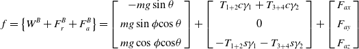 \begin{align}f = \left\{ {{W^B} + F_r^B + F_a^B} \right\} = \left[ {\begin{array}{c}{ - mg\;{\rm{sin}}\;\theta }\\[5pt] {mg\;{\rm{sin}}\;\phi {\rm{cos}}\;\theta }\\[5pt] {mg\;{\rm{cos}}\;\phi {\rm{cos}}\theta } \end{array}} \right] + \left[ {\begin{array}{c}{{T_{1 + 2}}c{\gamma _1} + {T_{3 + 4}}c{\gamma _2}}\\[5pt] 0\\[5pt] { - {T_{1 + 2}}s{\gamma _1} - {T_{3 + 4}}s{\gamma _2}}\end{array}} \right] + \left[ {\begin{array}{c}{{F_{ax}}}\\[5pt] {{F_{ay}}}\\[5pt] {{F_{az}}}\end{array}} \right]\end{align}
After developing the total force and moment acting on the CSF-TRUAV, the dynamics of the transnational motion of the drone are
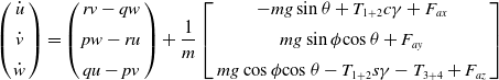 \begin{align}\left( {\begin{array}{c}{\dot u}\\[5pt] {\dot v}\\[5pt] {\dot w}\end{array}} \right) = \left( {\begin{array}{c}{rv - qw}\\[5pt] {pw - ru}\\[5pt] {qu - pv}\end{array}} \right) + \frac{1}{m}\left[ {\begin{array}{c}{ - mg\;{\rm{sin}}\;\theta + {T_{1 + 2}}c\gamma + {F_{ax}}}\\[5pt] {mg\;{\rm{sin}}\;\phi {\rm{cos}}\;\theta + {F_{ay}}}\\[5pt] {mg\;{\rm{cos}}\;\phi {\rm{cos}}\;\theta - {T_{1 + 2}}s\gamma - {T_{3 + 4}} + {F_{az}}}\end{array}} \right]\end{align}
This gives after transformation to the inertial frame:
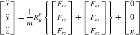 \begin{align}\left[ {\begin{array}{c}{\ddot x}\\[5pt] {\ddot y}\\[5pt] {\ddot z}\end{array}} \right] = \frac{1}{m}R_B^E\left\{ {\left[ {\begin{array}{c}{{F_{rx}}}\\[5pt] {{F_{ry}}}\\[5pt] {{F_{rz}}}\end{array}} \right] + \left[ {\begin{array}{c}{{F_{ax}}}\\[5pt] {{F_{ay}}}\\[5pt] {{F_{az}}}\end{array}} \right]} \right\} + \left[ {\begin{array}{c}0\\[5pt] 0\\[5pt] g\end{array}} \right]\end{align}
The rotational dynamics of the CSF-TRUAV are governed by
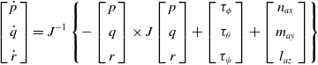 \begin{align}\left[ {\begin{array}{c}{\dot p}\\[5pt] {\dot q}\\[5pt] {\dot r}\end{array}} \right] = {J^{ - 1}}\left\{ { - \left[ {\begin{array}{c}p\\[5pt] q\\[5pt] r\end{array}} \right] \times J\left[ {\begin{array}{c}p\\[5pt] q\\[5pt] r\end{array}} \right] + \left[ {\begin{array}{c}{{\tau _\phi }}\\[5pt] {{\tau _\theta }}\\[5pt] {{\tau _\psi }}\end{array}} \right] + \left[ {\begin{array}{c}{{n_{ax}}}\\[5pt] {{m_{ay}}}\\[5pt] {{l_{az}}}\end{array}} \right]} \right\}\end{align}
This gives, after development
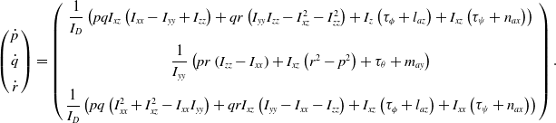 \begin{align}\left( {\begin{array}{c}{\dot p}\\[5pt] {\dot q}\\[5pt] {\dot r}\end{array}} \right) = \left( {\begin{array}{c}{\dfrac{1}{{{I_D}}}\left( {pq{I_{xz}}\left( {{I_{xx}} - {I_{yy}} + {I_{zz}}} \right) + qr\left( {{I_{yy}}{I_{zz}} - I_{xz}^2 - I_{zz}^2} \right) + {I_z}\left( {{\tau _\phi } + {l_{az}}} \right) + {I_{xz}}\left( {{\tau _\psi } + {n_{ax}}} \right)} \right)}\\[12pt] {\dfrac{1}{{{I_{yy}}}}\left( {pr\left( {{I_{zz}} - {I_{xx}}} \right) + {I_{xz}}\left( {{r^2} - {p^2}} \right) + {\tau _\theta } + {m_{ay}}} \right)}\\[12pt] {\dfrac{1}{{{I_D}}}\left( {pq\left( {I_{xx}^2 + I_{xz}^2 - {I_{xx}}{I_{yy}}} \right) + qr{I_{xz}}\left( {{I_{yy}} - {I_{xx}} - {I_{zz}}} \right) + {I_{xz}}\left( {{\tau _\phi } + {l_{az}}} \right) + {I_{xx}}\left( {{\tau _\psi } + {n_{ax}}} \right)} \right)}\end{array}} \right).\end{align}
with ${I_D} = {I_{xx}}{I_{zz}} - I_{xz}^2$
.
${I_D} = {I_{xx}}{I_{zz}} - I_{xz}^2$
.
4.0 Control strategy
This section describes the proposed control strategy and the derivation of the associated nonlinear controller, designed using a backstepping approach. Since the model of the CSF-TRUAV is highly nonlinear and coupled, some simplifying assumptions are considered to facilitate the controller design. Indeed, the nonlinearity and coupling of the CSF-TRUAV are more important compared to both multirotor and fixed-wing models.
Unlike classical multirotor drones, however, the CSF-TRUAV has an additional control input: the tilt angle of the front rotors. In the proposed control strategy, depicted in Fig. 7, this input is exploited to decouple the control of the forward position from the pitch angle. The desired trajectory of the CSF-TRUAV will hence be defined by five independent variables: the 3D position $\left( {{x^{\rm{*}}},{y^{\rm{*}}},{z^{\rm{*}}}} \right)$
in addition to the pitch and yaw angles
$\left( {{x^{\rm{*}}},{y^{\rm{*}}},{z^{\rm{*}}}} \right)$
in addition to the pitch and yaw angles $\left( {{\theta ^{\rm{*}}},{\psi ^{\rm{*}}}} \right)$
.
$\left( {{\theta ^{\rm{*}}},{\psi ^{\rm{*}}}} \right)$
.
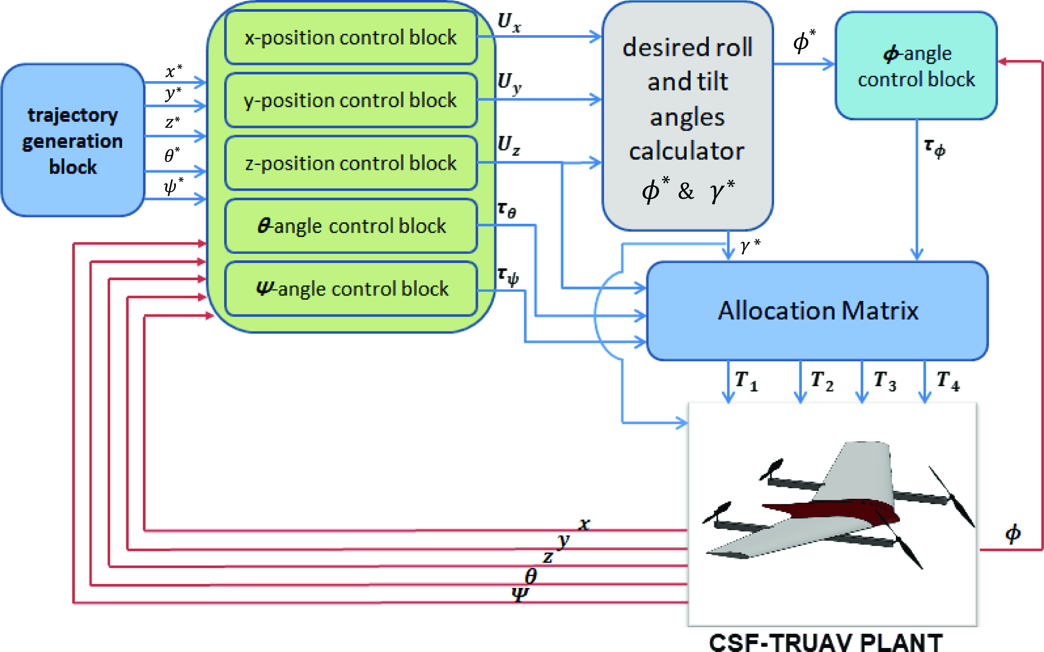
Figure 7. Proposed CSF-TRUAV control strategy.
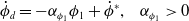
In this solution, the virtual control input ${U_x}$
generated by the forward position
${U_x}$
generated by the forward position $\left( x \right)$
controller is mapped to the tilt angle
$\left( x \right)$
controller is mapped to the tilt angle $\gamma $
. The drop in the vertical thrust force, caused by the tilting of the front rotors, is compensated for by increasing the rotation speed of these rotors in such a way that the projection of the generated forces on the
$\gamma $
. The drop in the vertical thrust force, caused by the tilting of the front rotors, is compensated for by increasing the rotation speed of these rotors in such a way that the projection of the generated forces on the $z$
axis satisfies the control output
$z$
axis satisfies the control output ${U_z}$
– the output of the altitude controller.
${U_z}$
– the output of the altitude controller.
The virtual control input ${U_y}$
is mapped to the roll angle
${U_y}$
is mapped to the roll angle ${\phi ^{\rm{*}}}$
in a similar way to a classical multirotor. The heading angle,
${\phi ^{\rm{*}}}$
in a similar way to a classical multirotor. The heading angle, ${\psi ^{\rm{*}}}$
, is also controlled like in a multirotor, by adjusting the difference between the average speed of the rotors rotating clockwise and the speed of those rotating anti-clockwise. The pitch angle, on the other hand, is controlled through the difference between the thrust forces of the rear rotors and the projection of the forces generated by the front rotors on the
${\psi ^{\rm{*}}}$
, is also controlled like in a multirotor, by adjusting the difference between the average speed of the rotors rotating clockwise and the speed of those rotating anti-clockwise. The pitch angle, on the other hand, is controlled through the difference between the thrust forces of the rear rotors and the projection of the forces generated by the front rotors on the ${z_b}$
axis.
${z_b}$
axis.
Unlike previous works, the proposed control strategy uses a single controller for both VTOL and cruise flight modes. Furthermore, this strategy exploits only the four rotors, and no control surfaces are needed.
The model derived in Section 3 is not suitable for control design. In fact, this model is too complex to provide meaningful insight into the drone’s motion. Furthermore, it presents a high degree of nonlinearity and coupling between state variables. To simplify this model, the following assumptions are considered:
-
The roll
$\phi $
and pitch
$\theta $
angles are small, so Equation (6) can be simplified to(27)
\begin{align}\left( {\begin{array}{c}{\dot \phi }\\[5pt] {\dot \theta }\\[5pt] {\dot \psi }\end{array}} \right) = \left( {\begin{array}{c}p\\[5pt] q\\[5pt] r\end{array}} \right)\end{align}
-
Given the symmetry of the CSF-TRUAV in the
$xz$
plan, the term
${I_{xz}}$
in the inertia matrix is neglected. This simplifies Equation (26) to(28)
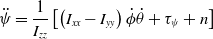
\begin{align}\left( {\begin{array}{c}{\ddot \phi }\\[5pt] {\ddot \theta }\\[5pt] {\ddot \psi }\end{array}} \right) = \left( {\begin{array}{c}{\dfrac{{{I_{yy}} - {I_{zz}}}}{{{I_{xx}}}}\dot \theta \dot \psi + \dfrac{{{\tau _\phi } + l}}{{{I_{xx}}}}}\\[12pt] {\dfrac{{{I_{zz}} - {I_{xx}}}}{{{I_{yy}}}}\dot \phi \dot \psi + \dfrac{{{\tau _\theta } + m}}{{{I_{yy}}}}}\\[12pt] {\dfrac{{{I_{xx}} - {I_{yy}}}}{{{I_{zz}}}}\dot \phi \dot \theta + \dfrac{{{\tau _\psi } + n}}{{{I_{zz}}}}}\end{array}} \right)\end{align}


It is worth noting that these simplifications are only considered for controller design and that the full nonlinear model is used for simulating the dynamics of the CSF-TRUAV.
Without loss of generality, let us consider the control vector $U$
, such that
$U$
, such that
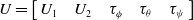 \begin{align}U = \left[ {\begin{array}{c@{\quad}c@{\quad}c@{\quad}c@{\quad}c}{{U_1}} & {{U_2}} & {{\tau _\phi }} & {{\tau _\theta }} & {{\tau _\psi }}\end{array}} \right]\end{align}
where:
-
${U_1}$
: the resultant upward force of the four rotors. It is the sum of the projection of the front rotors’ thrust forces onto the
${z_B}$
axis and the thrust forces of the two rear rotors. This control input is mapped to the drone’s altitude,
$z$
, controller.(30)
\begin{align}{U_1} = - {T_{1 + 2}}{\rm{sin}}\;\gamma - {T_{3 + 4}}\end{align}
-
${U_2}$
: the projection of the two front rotors thrust forces onto the
${x_B}$
axis and it is responsible on the control of TRUAV’s forward position.(31)
\begin{align}{U_2} = {T_{1 + 2}}{\rm{cos}}\;\gamma \end{align}
-
${\tau _\phi }$
: this torque results from the difference between the thrust generated by the left rotors (2 and 4) and the right rotors (1 and 3). This input mainly affects the roll angle,
$\phi $
, and is hence mapped to the controller of this angle.(32)
\begin{align}{\tau _\phi } = \left( {{K_{ld}}{\rm{cos}}\;\gamma - {l_y}{\rm{sin}}\;\gamma } \right){T_{1 - 2}} - {l_y}{T_{3 - 4}}\end{align}
-
4.
${\tau _\theta }$
: this input depends on the tilt angle,
${\gamma _1}$
. It results from the difference between the thrust generated by the back rotors, and the projection of the thrust of the front rotors on the
${z_B}$
axis. This input is responsible for the control of the pitch angle,
$\theta $
.(33)
\begin{align}{\tau _\theta } = {\rm{sin}}\;\gamma {l_x}{T_{1 + 2}} - {l_x}{T_{3 + 4}}\end{align}
-
5.
${\tau _\psi }$
: the difference between the drag torque between the clockwise spinning rotors and the torque of the rotors spinning anticlockwise. This input controls the yaw angle
$\psi $
.(34)
\begin{align}{\tau _\psi } = - \left( {{K_{ld}}{\rm{sin}}\;\gamma + {l_y}{\rm{cos}}\;\gamma } \right){T_{1 - 2}} + {K_{ld}}{T_{3 - 4}}\end{align}


After introducing the above simplifying assumptions and substituting the control input vector $U$
in Equations (24) and (26), the CSF-TRUAV’s control-model becomes:
$U$
in Equations (24) and (26), the CSF-TRUAV’s control-model becomes:
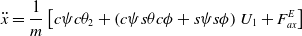 \begin{align}\ddot x = \frac{1}{m}\left[ {c\psi c{\theta _2} + \left( {c\psi s\theta c\phi + s\psi s\phi } \right){U_1} + F_{ax}^E} \right]\end{align}
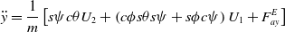 \begin{align}\ddot y = \frac{1}{m}\left[ {s\psi c\theta {U_2} + \left( {c\phi s\theta s\psi + s\phi c\psi } \right){U_1} + F_{ay}^E} \right]\end{align}
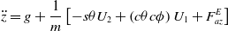 \begin{align}\ddot z = g + \frac{1}{m}\left[ { - s\theta {U_2} + \left( {c\theta c\phi } \right){U_1} + F_{az}^E} \right]\end{align}
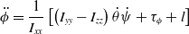 \begin{align}\ddot \phi = \frac{1}{{{I_{xx}}}}\left[ {\left( {{I_{yy}} - {I_{zz}}} \right)\dot \theta \dot \psi + {\tau _\phi } + l} \right]\end{align}
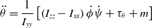 \begin{align}\ddot \theta = \frac{1}{{{I_{yy}}}}\left[ {\left( {{I_{zz}} - {I_{xx}}} \right)\dot \phi \dot \psi + {\tau _\theta } + m} \right]\end{align}
 \begin{align}\ddot \psi = \frac{1}{{{I_{zz}}}}\left[ {\left( {{I_{xx}} - {I_{yy}}} \right)\dot \phi \dot \theta + {\tau _\psi } + n} \right]\end{align}
To facilitate controller design, the following intermediate control variables are considered, which are the outputs of three SISO position controllers
 \begin{align}{U_x} = c\psi c\theta {U_2} + \left( {c\psi s\theta c\phi + s\psi s\phi } \right){U_1}\end{align}
 \begin{align}{U_y} = s\psi c\theta {U_2} + \left( {c\phi s\theta s\psi - s\phi c\psi } \right){U_1}\end{align}
 \begin{align}{U_z} = - s\theta {U_2} + \left( {c\phi c\theta } \right){U_1}\end{align}
Equations (41), (42) and (43) can be simplified then arranged in a matrix form as
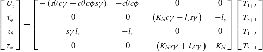 \begin{align}\left[ {\begin{array}{c}{{U_z}}\\[5pt] {{\tau _\phi }}\\[5pt] {{\tau _\theta }}\\[5pt] {{\tau _\psi }}\end{array}} \right] = \left[ {\begin{array}{c@{\quad}c@{\quad}c@{\quad}c}{ - \left( {s\theta c\gamma + c\theta c\phi s\gamma } \right)} & { - c\theta c\phi }& 0 &0\\[5pt] 0 & 0 & {\left( {{K_{ld}}c\gamma - {l_y}s\gamma } \right)} & { - {l_y}}\\[5pt] {s\gamma {l_x}} & { - {l_x}} & 0 & 0\\[5pt] 0 & 0 & { - \left( {{K_{ld}}s\gamma + {l_y}c\gamma } \right)} & {{K_{ld}}}\end{array}} \right]\left[ {\begin{array}{c}{{T_{1 + 2}}}\\[5pt] {{T_{3 + 4}}}\\[5pt] {{T_{1 - 2}}}\\[5pt] {{T_{3 - 4}}}\end{array}} \right]\end{align}
By inverting the allocation matrix in Equation (44) the thrust forces are calculated as
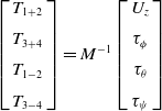 \begin{align}\left[ {\begin{array}{c}{{T_{1 + 2}}}\\[5pt] {{T_{3 + 4}}}\\[5pt] {{T_{1 - 2}}}\\[5pt] {{T_{3 - 4}}}\end{array}} \right] = {M^{ - 1}}\left[ {\begin{array}{c}{{U_z}}\\[5pt] {{\tau _\phi }}\\[5pt] {{\tau _\theta }}\\[5pt] {{\tau _\psi }}\end{array}} \right]\end{align}
with ${M^{ - 1}}$
given by
${M^{ - 1}}$
given by
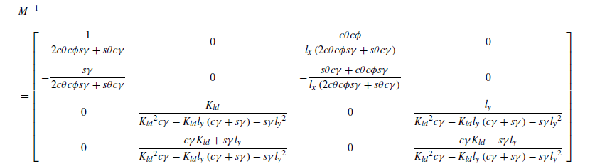 \begin{align} & {M^{ - 1}} \nonumber \\[5pt] &= \left[\begin{array}{c@{\quad}c@{\quad}c@{\quad}c} { - \dfrac{1}{{2c\theta c\phi s\gamma + s\theta c\gamma }}} & 0 & {\dfrac{{c\theta c\phi }}{{{l_x}\left( {2c\theta c\phi s\gamma + s\theta c\gamma } \right)}}} & 0\\[12pt] { - \dfrac{{s\gamma }}{{2c\theta c\phi s\gamma + s\theta c\gamma }}} & 0 & { - \dfrac{{s\theta c\gamma + c\theta c\phi s\gamma }}{{{l_x}\left( {2c\theta c\phi s\gamma + s\theta c\gamma } \right)}}} & 0\\[12pt] 0 & {\dfrac{{{K_{ld}}}}{{{K_{ld}}^2c\gamma - {K_{ld}}{l_y}\left( {c\gamma + s\gamma } \right) - s\gamma {l_y}^2}}} & 0 & {\dfrac{{{l_y}}}{{{K_{ld}}^2c\gamma - {K_{ld}}{l_y}\left( {c\gamma + s\gamma } \right) - s\gamma {l_y}^2}}}\\[12pt] 0 & {\dfrac{{c\gamma {K_{ld}} + s\gamma {l_y}}}{{{K_{ld}}^2c\gamma - {K_{ld}}{l_y}\left( {c\gamma + s\gamma } \right) - s\gamma {l_y}^2}}} & 0 & {\dfrac{{c\gamma {K_{ld}} - s\gamma {l_y}}}{{{K_{ld}}^2c\gamma - {K_{ld}}{l_y}\left( {c\gamma + s\gamma } \right) - s\gamma {l_y}^2}}}\end{array} \right]\end{align}
The desired rotors’ velocities are calculated from the intermediate variables ${T_{1 + 2}},{T_{1 - 2}}$
,
${T_{1 + 2}},{T_{1 - 2}}$
, ${T_{3 + 2}},{T_{3 - 4}}$
as
${T_{3 + 2}},{T_{3 - 4}}$
as
 \begin{align}{{\rm{\Omega }}_1} = \sqrt {\frac{{{T_{1 + 2}} + {T_{1 - 2}}}}{{2{K_{ld}}}}} \end{align}
 \begin{align}{{\rm{\Omega }}_2} = \sqrt {\frac{{{T_{1 + 2}} - {T_{1 - 2}}}}{{2{K_{ld}}}}} \end{align}
 \begin{align}{{\rm{\Omega }}_3} = \sqrt {\frac{{{T_{3 + 4}} + {T_{3 - 4}}}}{{2{K_{ld}}}}} \end{align}
 \begin{align}{{\rm{\Omega }}_4} = \sqrt {\frac{{{T_{3 + 4}} + {T_{3 - 4}}}}{{2{K_{ld}}}}} \end{align}
To determine the desired roll ${\phi ^{\rm{*}}}$
and tilt
${\phi ^{\rm{*}}}$
and tilt ${\gamma ^{\rm{*}}}$
angles, Equation (41) is multiplied by
${\gamma ^{\rm{*}}}$
angles, Equation (41) is multiplied by ${\rm{cos}}\;\psi $
and Equation (42) by
${\rm{cos}}\;\psi $
and Equation (42) by ${\rm{sin}}\;\psi $
. This gives after summation
${\rm{sin}}\;\psi $
. This gives after summation
 \begin{align}{U_x}c\psi + {U_z}s\psi = {U_2}c\theta + {U_1}s\theta c\phi \end{align}
If one further multiplies Equation (51) by $s\theta $
and Equation (43) by
$s\theta $
and Equation (43) by $c\theta $
, one can write
$c\theta $
, one can write ${U_1}$
in terms of the control outputs
${U_1}$
in terms of the control outputs ${U_x}$
,
${U_x}$
, ${U_y}$
, and
${U_y}$
, and ${U_z}$
as
${U_z}$
as
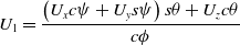 \begin{align}{U_1} = \frac{{\left( {{U_x}c\psi + {U_y}s\psi } \right)s\theta + {U_z}c\theta }}{{c\phi }}\end{align}
Multiplying ${U_x}$
by
${U_x}$
by $s\psi $
and
$s\psi $
and ${U_y}$
by
${U_y}$
by $c\psi $
in Equations (41) and (42) one can write
$c\psi $
in Equations (41) and (42) one can write
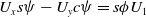 \begin{align}{U_x}s\psi - {U_y}c\psi = s\phi {U_1}\end{align}
Combining Equations (52) and (53), the reference for the roll angle, ${\phi ^{\rm{*}}}$
, is calculated as
${\phi ^{\rm{*}}}$
, is calculated as
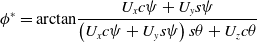 \begin{align}{\phi ^{\rm{*}}} = {\rm{arctan}}\frac{{{U_x}c\psi + {U_y}s\psi }}{{\left( {{U_x}c\psi + {U_y}s\psi } \right)s\theta + {U_z}c\theta }}\end{align}
Multiplying Equation (51) by $c\theta $
and Equation (43) by
$c\theta $
and Equation (43) by $s\theta $
,
$s\theta $
, ${U_2}$
can be expressed in terms of the control outputs
${U_2}$
can be expressed in terms of the control outputs ${U_x}$
,
${U_x}$
, ${U_y}$
, and
${U_y}$
, and ${U_z}$
as
${U_z}$
as
 \begin{align}{U_2} = \left( {{U_x}c\psi + {U_y}s\psi } \right)c\theta - {U_z}s\theta \end{align}
The reference for the tilt angle, ${\gamma ^{\rm{*}}}$
, is calculated from Equations (31) and (55), as
${\gamma ^{\rm{*}}}$
, is calculated from Equations (31) and (55), as
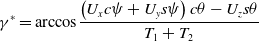 \begin{align}{\gamma ^{\rm{*}}} = {\rm{arccos}}\frac{{\left( {{U_x}c\psi + {U_y}s\psi } \right)c\theta - {U_z}s\theta }}{{{T_1} + {T_2}}}\end{align}
Given the afore-described control strategy, the design of the controllers that yield the reference values for the variables ${U_x}$
,
${U_x}$
, ${U_y}$
,
${U_y}$
, ${U_z}$
,
${U_z}$
, ${\tau _\phi }$
,
${\tau _\phi }$
, ${\tau _\theta }$
and
${\tau _\theta }$
and ${\tau _\psi }$
is presented in what follows.
${\tau _\psi }$
is presented in what follows.
Let us start with the tracking of the roll angle, $\phi $
. For the sake of clarity, the dynamics for this variable are written in the following form:
$\phi $
. For the sake of clarity, the dynamics for this variable are written in the following form:
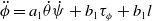 \begin{align}\ddot \phi = {a_1}\dot \theta \dot \psi + {b_1}{\tau _\phi } + {b_1}l\end{align}
with
 \begin{align}{a_1} = \frac{{{I_{yy}} - {I_{zz}}}}{{{I_{xx}}}},{\rm{\;\;\;\;\;\;\;\;}}{b_1} = \frac{1}{{{I_{xx}}}}\end{align}
Let ${\phi _1}$
,
${\phi _1}$
, ${\dot \phi _1}$
respectively denote the tracking error for the roll angle and its time derivative
${\dot \phi _1}$
respectively denote the tracking error for the roll angle and its time derivative
 \begin{align}{\phi _1} = \phi - {\phi ^{\rm{*}}};{\rm{\;\;\;\;}}{\dot \phi _1} = \dot \phi - {\dot \phi ^{\rm{*}}}\end{align}
If one further chooses the Lyapunov function ${V_1}$
such that
${V_1}$
such that
 \begin{align}{V_1} = \frac{1}{2}\phi _1^2\end{align}
The time derivative of ${V_1}$
is
${V_1}$
is
 \begin{align}{\dot V_1} = {\phi _1}{\dot \phi _1} = {\phi _1}\left( {\dot \phi - {{\dot \phi }^{\rm{*}}}} \right)\end{align}
To ensure that the roll rate $\dot \phi $
converge asymptotically, the derivative
$\dot \phi $
converge asymptotically, the derivative ${\dot V_1}$
must be negative semi definite. Because the roll rate,
${\dot V_1}$
must be negative semi definite. Because the roll rate, $\dot \phi $
, is not a control input, it is considered a virtual input and the following reference is defined for it
$\dot \phi $
, is not a control input, it is considered a virtual input and the following reference is defined for it
 \begin{align}{\dot \phi _d} = - {\alpha _{{\phi _1}}}{\phi _1} + {\dot \phi ^{\rm{*}}},{\rm{\;\;\;\;}}{\alpha _{{\phi _1}}} \gt 0\end{align}
To ensure the tracking of this reference, the following tracking error is considered
 \begin{align}{\phi _2} = \dot \phi - {\dot \phi _d} = \dot \phi - {\dot \phi ^{\rm{*}}} + {\alpha _{{\phi _1}}}{\phi _1}\end{align}
The rate of change of this error is
 \begin{align}{\dot \phi _2} = {a_1}\dot \theta \dot \psi + {b_1}{\tau _\phi } + {b_1}l + {\alpha _{{\phi _1}}}\left( {\dot \phi - {{\dot \phi }^{\rm{*}}}} \right) - {\ddot \phi ^{\rm{*}}}\end{align}
To ensure an asymptotic convergence of ${\phi _2}$
, the following Lyaponuv function is considered
${\phi _2}$
, the following Lyaponuv function is considered
 \begin{align}{V_2} = {V_1} + \frac{1}{2}\phi _2^2\end{align}
The temporal derivative of ${V_2}$
is
${V_2}$
is
 \begin{align}{\dot V_2} = {\dot V_1} + {\phi _2}{\dot \phi _2}\end{align}
 \begin{align} = {\phi _1}\left( {{\phi _2} + {{\dot \phi }_d} - {{\dot \phi }^{\rm{*}}}} \right) + {\phi _2}\left( {\dot \theta \dot \psi {a_1} + {b_1}{\tau _\phi } + {b_1}l + {\alpha _{{\phi _1}}}\left( {\dot \phi - {{\dot \phi }^{\rm{*}}}} \right) - {{\ddot \phi }^{\rm{*}}}} \right)\end{align}
 \begin{align} = - {k_1}\phi _1^2 + {\phi _2}\left( {\dot \theta \dot \psi {a_1} + {b_1}{\tau _\phi } + {b_1}l + {\alpha _{{\phi _1}}}\left( { - {\alpha _{{\phi _1}}}{\phi _1} + {\phi _2}} \right) - {{\ddot \phi }^{\rm{*}}} + {\phi _1}} \right)\end{align}
To satisfy the condition of asymptotic stability, $\dot V\left( {{\phi _1},{\phi _2}} \right) \lt 0$
, the control input
$\dot V\left( {{\phi _1},{\phi _2}} \right) \lt 0$
, the control input ${\tau _\phi }$
is chosen such that
${\tau _\phi }$
is chosen such that
 \begin{align}{\tau _\phi } = \frac{1}{{{b_1}}}\left( { - {a_1}\dot \theta \dot \psi - {b_1}l + {{\ddot \phi }^{\rm{*}}} - {\alpha _{{\phi _1}}}\left( { - {\alpha _{{\phi _1}}}{\phi _1} + {\phi _2}} \right) - {\phi _1} - {\alpha _{{\phi _2}}}{\phi _2}} \right){\rm{\;\;\;\;}}{\alpha _{{\phi _2}}} \gt 0\end{align}
Following the same previous steps, the control inputs ${\tau _\theta }$
,
${\tau _\theta }$
, ${\tau _\psi }$
,
${\tau _\psi }$
, ${U_z}$
,
${U_z}$
, ${U_x}$
and
${U_x}$
and ${U_y}$
are calculated as
${U_y}$
are calculated as
 \begin{align}{\tau _\theta } = \frac{1}{{{b_2}}}\left( { - {a_2}\dot \phi \dot \psi - {b_2}m + {{\ddot \theta }^{\rm{*}}} - {\alpha _{{\theta _1}}}\left( { - {\alpha _{{\theta _1}}}{\theta _1} + {\theta _2}} \right) - {\theta _1} - {\alpha _{{\theta _2}}}{\theta _2}} \right)\end{align}
 \begin{align}{\tau _\psi } = \frac{1}{{{b_3}}}\left( { - {a_3}\dot \phi \dot \theta - {b_3}n + {{\ddot \psi }^{\rm{*}}} - {\alpha _{{\psi _1}}}\left( { - {\alpha _{{\psi _1}}}{\psi _1} + {\psi _2}} \right) - {\psi _1} - {\alpha _{{\psi _2}}}{\psi _2}} \right)\end{align}
 \begin{align}{U_z} = m\left( { - g - \frac{{F_{az}^i}}{m} + {{\ddot z}^{\rm{*}}} - {\alpha _{{z_1}}}\left( { - {k_7}{z_1} + {z_2}} \right) - {z_1} - {\alpha _{{z_2}}}{z_2}} \right)\end{align}
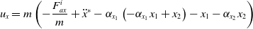 \begin{align}{u_x} = m\left( { - \frac{{F_{ax}^i}}{m} + {{\ddot x}^{\rm{*}}} - {\alpha _{{x_1}}}\left( { - {\alpha _{{x_1}}}{x_1} + {x_2}} \right) - {x_1} - {\alpha _{{x_2}}}{x_2}} \right)\end{align}
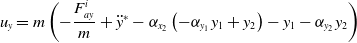 \begin{align}{u_y} = m\left( { - \frac{{F_{ay}^i}}{m} + {{\ddot y}^{\rm{*}}} - {\alpha _{{x_2}}}\left( { - {\alpha _{{y_1}}}{y_1} + {y_2}} \right) - {y_1} - {\alpha _{{y_2}}}{y_2}} \right)\end{align}
with
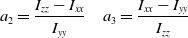 \begin{align*}{\rm{\;\;\;\;}}{a_2} = \frac{{{I_{zz}} - {I_{xx}}}}{{{I_{yy}}}}\quad {a_3} = \frac{{{I_{xx}} - {I_{yy}}}}{{{I_{zz}}}}\end{align*}
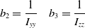 \begin{align*}{b_2} = \frac{1}{{{I_{yy}}}}\quad {b_3} = \frac{1}{{{I_{zz}}}}\end{align*}
and the tracking errors for the six DOF of the CSF-TRUAV defined as:
 \begin{align*}{\rm{\;\;\;\;}}{\theta _1} = \theta - {\theta ^{\rm{*}}}{\theta _2} = \dot \theta - {\dot \theta ^{\rm{*}}} + {\alpha _{{\theta _1}}}{\theta _1}\end{align*}
 \begin{align*}{\psi _1} = \psi - {\psi ^{\rm{*}}}{\psi _2} = \dot \psi - {\dot \psi ^{\rm{*}}} + {\alpha _{{\psi _1}}}{\psi _1}\end{align*}
 \begin{align*}{z_1} = z - {z^{\rm{*}}}{z_2} = \dot z - {\dot z^{\rm{*}}} + {\alpha _{{z_1}}}{z_1}\end{align*}
 \begin{align*}{x_1} = x - {x^{\rm{*}}}{x_2} = \dot x - {\dot x^{\rm{*}}} + {\alpha _{{x_1}}}{x_1}\end{align*}
 \begin{align*}{y_1} = y - {y^{\rm{*}}}{y_2} = \dot y - {\dot y^{\rm{*}}} + {\alpha _{{y_1}}}{y_1},\end{align*}
5.0 Results and discussion
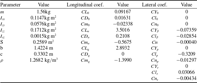
To validate the proposed control strategy and the designed backstepping controller, several scenarios are simulated in this section. The model considered in this work is that of the famous Zagi flying wing illustrated in Fig. 8. The geometrical, inertial and aerodynamic parametres of this drone are summarised in Table 1.
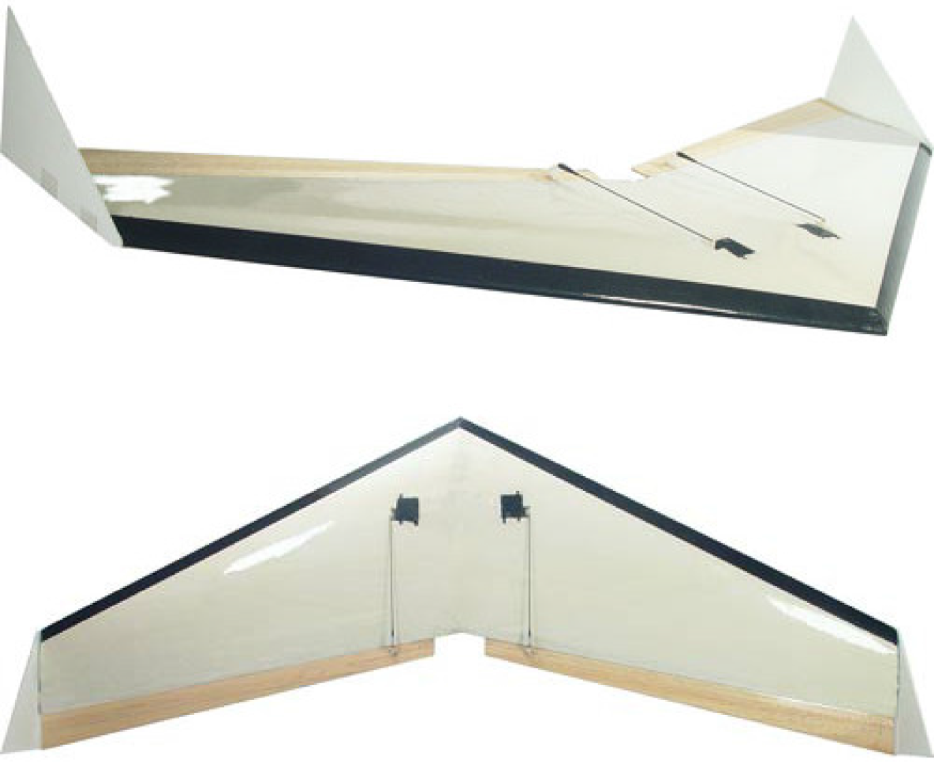
Figure 8. The Zagi flying wing drone whose model is used in this work.
To make this model even more realistic, a saturation of the four actuators is considered. The saturation is chosen in such a way that the four rotors can only ensure a total lift force of two times the weight of the drone. Half of this force compensates for the drone’s weight while in VTOL mode. The other half is used for vertical manoeuvres and to compensate for the drop in vertical thrust caused by the tilt of the front rotors.
The validation trajectory is composed of three phases. The first is a takeoff and vertical flight to an altitude of 7.5m. In the second phase, the drone pitches up and accelerates in the forward direction until it achieves a speed of 7m/s, which it maintains for 20s. The drone then starts decelerating until it comes to a stop, where it levels out and then starts landing. The reference trajectory is described by the following equations:
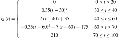 \begin{align}{x_d}\left( t \right) = \left\{ {\begin{array}{c@{\quad}c}0 & {0 \le t \le 20}\\[5pt] {0.35{{(t - 30)}^2}} & {30 \le t \le 40}\\[5pt] {7\left( {t - 40} \right) + 35} & {40 \le t \le 60}\\[5pt] { - 0.35{{(t - 60)}^2} + 7\left( {t - 60} \right) + 175} & {60 \le t \le 70}\\[5pt] {210} & {70 \le t \le 100}\end{array}} \right.\end{align}
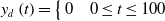 \begin{align}{y_d}\left( t \right) = \left\{ {\begin{array}{c@{\quad}c}0 & {0 \le t \le 100} \end{array}} \right.\end{align}
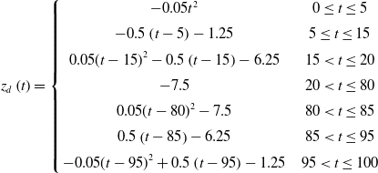 \begin{align}{z_d}\left( t \right) = \left\{ {\begin{array}{c@{\quad}c}{ - 0.05{t^2}} & {0 \le t \le 5}\\[5pt] { - 0.5\left( {t - 5} \right) - 1.25} & {5 \le t \le 15}\\[5pt] {0.05{{(t - 15)}^2} - 0.5\left( {t - 15} \right) - 6.25} & {15 \lt t \le 20}\\[5pt] { - 7.5} & {20 \lt t \le 80}\\[5pt] {0.05{{(t - 80)}^2} - 7.5} & {80 \lt t \le 85}\\[5pt] {0.5\left( {t - 85} \right) - 6.25} & {85 \lt t \le 95}\\[5pt] { - 0.05{{(t - 95)}^2} + 0.5\left( {t - 95} \right) - 1.25} & {95 \lt t \le 100}\end{array}} \right.\end{align}
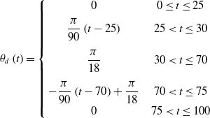 \begin{align}{\theta _d}\left( t \right) = \left\{ {\begin{array}{c@{\quad}c}0 & {0 \le t \le 25}\\[5pt] {\dfrac{\pi }{{90}}\left( {t - 25} \right)} & {25 \lt t \le 30}\\[12pt] {\dfrac{\pi }{{18}}} & {30 \lt t \le 70}\\[12pt] { - \dfrac{\pi }{{90}}\left( {t - 70} \right) + \dfrac{\pi }{{18}}} & {70 \lt t \le 75}\\[5pt] 0 & {75 \lt t \le 100}\end{array}} \right.\end{align}
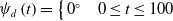 \begin{align}{\psi _d}\left( t \right) = \left\{ {\begin{array}{c@{\quad}c}{{0^ \circ }} & {0 \le t \le 100}\end{array}} \right.\end{align}
Regarding the trim condition, the angle-of-attack was arbitrarily set to ${10^{\rm{o}}}$
in the simulation scenario. For an optimal exploitation of the available energy, the trimming point has to be chosen in such a way as to maximise the lift force. Unlike conventional designs, aerodynamic stability is not an issue in the CSF-TRUAV since it is controlled using only propellers.
${10^{\rm{o}}}$
in the simulation scenario. For an optimal exploitation of the available energy, the trimming point has to be chosen in such a way as to maximise the lift force. Unlike conventional designs, aerodynamic stability is not an issue in the CSF-TRUAV since it is controlled using only propellers.
Table 1. The Zagi flying wing parameters
In what follows, the obtained results for three simulation scenarios are discussed. In the first scenario, the control equations designed in the previous section are used, including the feed-forward compensation of the aerodynamic forces and moments.
In the second scenario, the terms related to the aerodynamic forces and moments are neglected in the control equations, given the difficulties related to the estimation of these terms. In the third scenario, an integral backstepping controller is considered to enhance the robustness against the neglected aerodynamic forces and moments.
5.1 First scenario: Backstepping control with feed-forward compensation of aerodynamic forces and moments
Figure 9 depicts the 3D reference path together with the path followed by the drone. As the figure shows, the proposed control strategy and designed backstepping controller allowed the CSF-TRUAV to accurately track the reference path during all the flight phases.
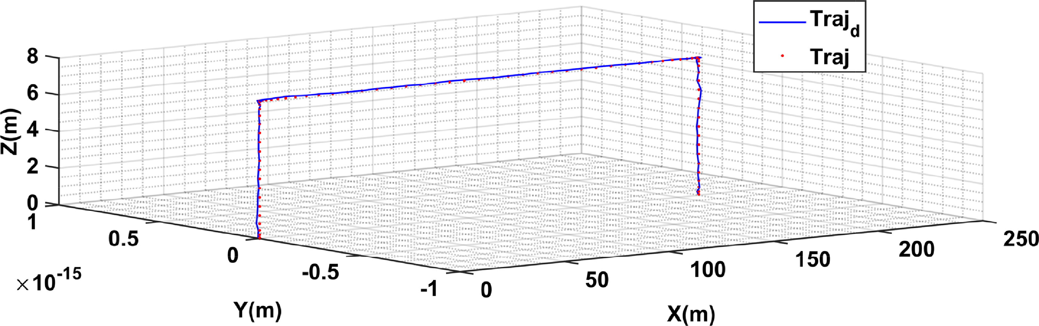
Figure 9. First scenario results: 3D path followed by the CSF-TRUAV.
Figure 10(a) illustrates in more detail the reference trajectory and the trajectory followed by the drone. The corresponding tracking errors are presented in Fig. 10(b). As can be noticed, the error is negligible for the y-axis during all the flight phases. This is due to the absence of manoeuvres along this axis. For the $x$
-axis, on the other hand, the error is more important, namely during the cruise flight and deceleration phases. The errors observed for the z-axis during the takeoff and landing phases are due to the accelerations performed during the two phases. The errors observed during the cruise flight phase are caused by the coupling between the x-axis and z-axis control.
$x$
-axis, on the other hand, the error is more important, namely during the cruise flight and deceleration phases. The errors observed for the z-axis during the takeoff and landing phases are due to the accelerations performed during the two phases. The errors observed during the cruise flight phase are caused by the coupling between the x-axis and z-axis control.
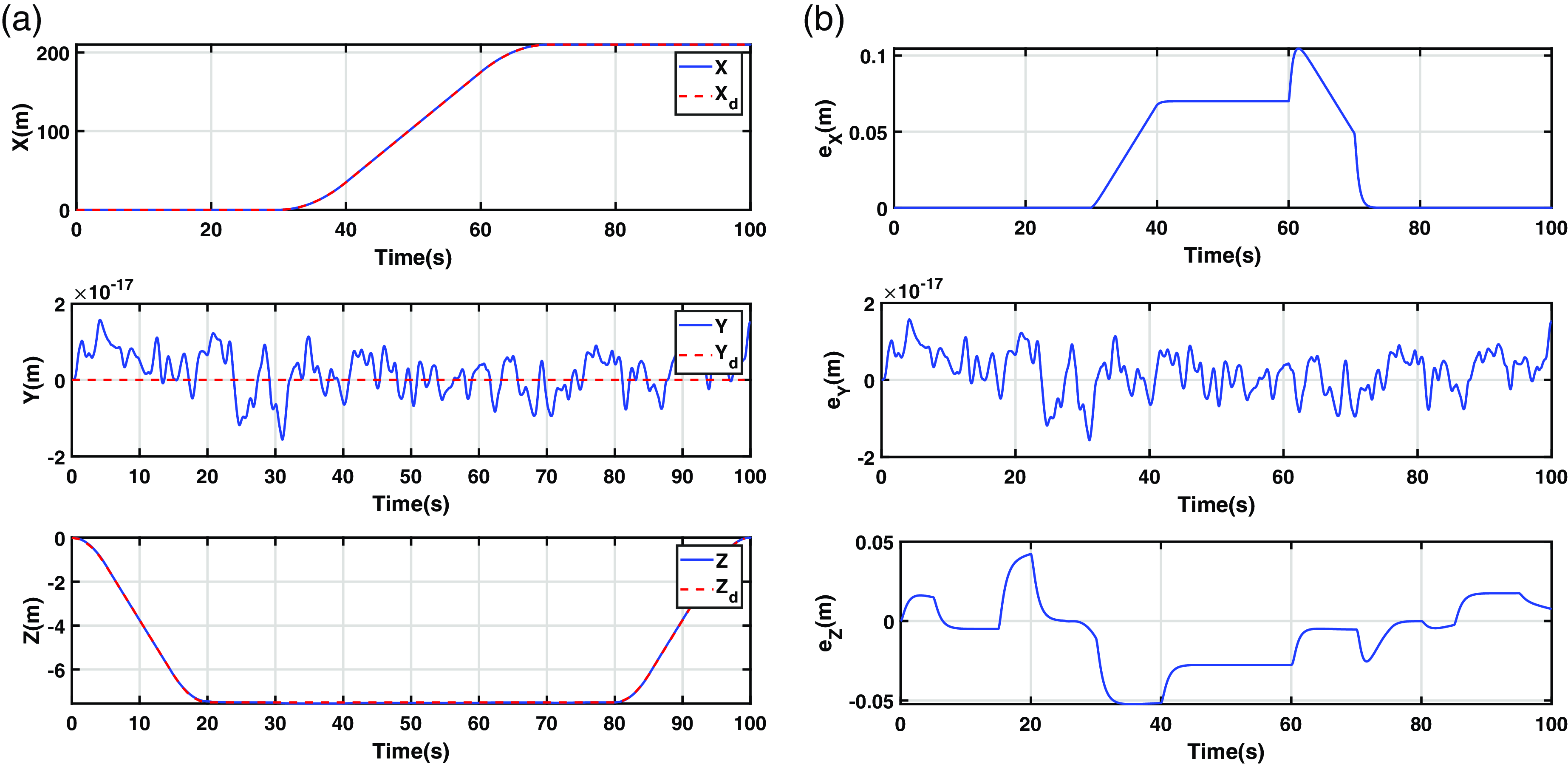
Figure 10. First scenario results: (a) desired and actual horizontal positions and altitude; (b) corresponding tracking errors.
Figure 11(a) shows the evolution of the drone’s attitude, while Fig. 11(b) is a plot of the corresponding tracking error. It is worth noting that the variations in the pitch angle did not affect the drone’s altitude or its forward position. This is due to the proposed control strategy, which decouples the control of the forward position from that of the pitch angle. Furthermore, the nonlinear nature of the controller allows taking into account any variation in the pitch angle. This means the effect of the pitch angle on the position is compensated implicitly by the controller.
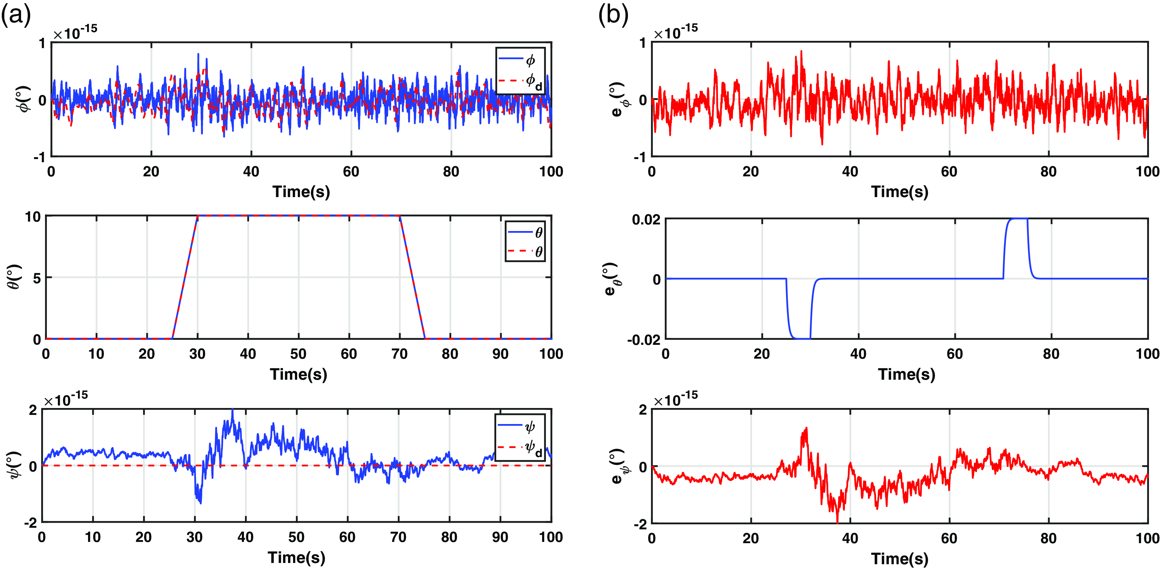
Figure 11. First scenario results: (a) desired and actual attitude of the CSF-TRUAV; (b) from top to bottom roll, pitch and heading tracking errors ${e_\psi }$
.
${e_\psi }$
.
Figure 12(a) illustrates the thrust forces generated by the four rotors. Note that the four control inputs remain within the limits of the actuators. As the drone gains speed in the forward direction, more lift is generated by the wings, and hence less demands are put on the actuators. This results in less energy consumption compared to a standard multirotor. In the cruise flight phase, the resultant aerodynamic lift generated by the wings reaches 5.6N, i.e. about 37% of the total lift. The differences observed between the back and front rotors are due to the tilting of the latter. In fact, any increase in the tilt angle causes a decrease in the vertical component of the thrust, which is compensated for by increasing the rotation speed of the front rotors.
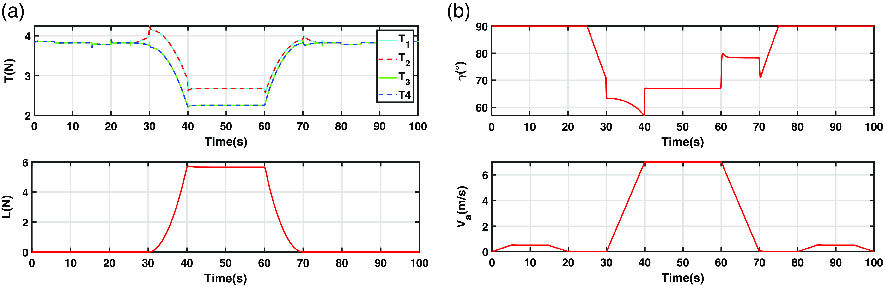
Figure 12. Results of the first scenario: (a) thrust and lift forces; (b) tilt angle and airspeed.
The maximum tilt angle attained in this scenario is around ${33^ \circ }$
from vertical (see Fig. 12(b)), which is far from the saturation of
${33^ \circ }$
from vertical (see Fig. 12(b)), which is far from the saturation of ${60^ \circ }$
that was set for this variable. Unlike previous works, this saturation is necessary for the proposed control scheme. The reason for this is the requirement for a minimum component of thrust on the
${60^ \circ }$
that was set for this variable. Unlike previous works, this saturation is necessary for the proposed control scheme. The reason for this is the requirement for a minimum component of thrust on the ${z_b}$
axis to allow controlling the pitch angle.
${z_b}$
axis to allow controlling the pitch angle.
5.2 Second scenario: Backstepping control without compensation for the aerodynamic forces and moments
As noted in the previous section, the aerodynamic forces generated by the wings compensate for the drone’s weight, resulting in better energy efficiency. From a control point of view, however, these forces and moments might be difficult to deal with. The first scenario assumed the availability of accurate measurements for these perturbations, which allowed their explicit compensation through feed-forward terms.
Such accurate measurements are difficult to get in practice, especially on a small-scale drone. This is due to the absence of the required sensors and the complexity of the estimation procedure. In fact, an accurate estimation requires precise measurements of airspeed, angle-of-attack and side sleep angle. It also hinges upon an accurate aerodynamic analysis of the drone at different flight conditions.
The purpose of the second scenario is to assess the performance of the control if the aerodynamic forces and moments are not considered. In this case, they will be treated as external disturbances. The effect of these perturbations on the drone trajectory is outlined in Figs. 13, 14, and 15.
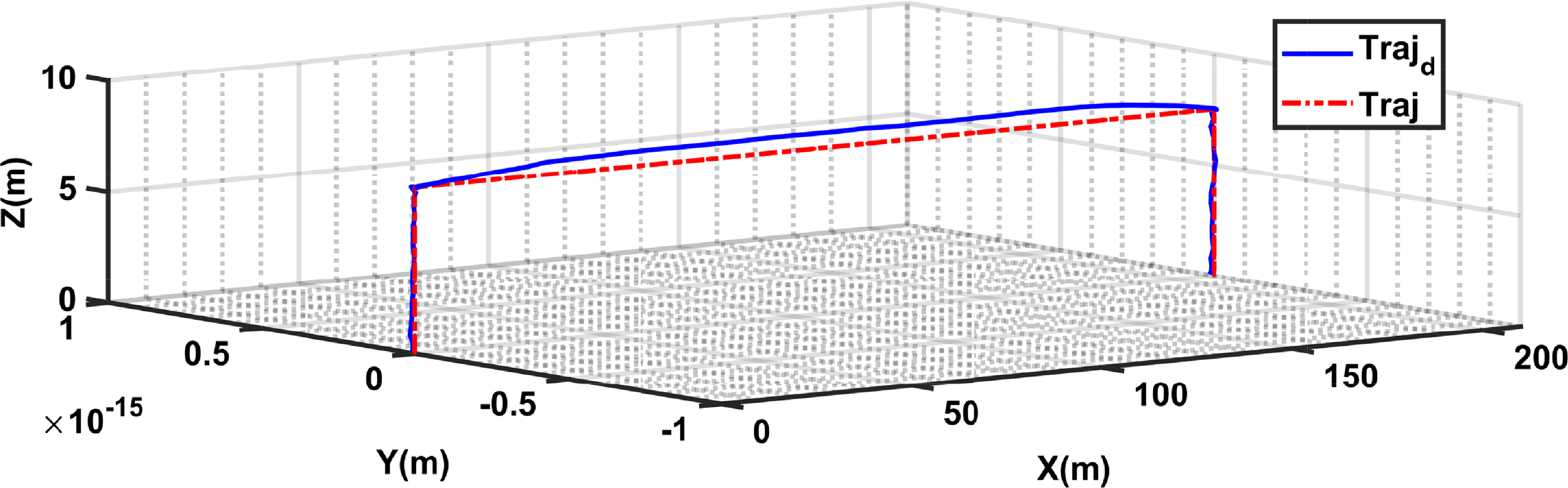
Figure 13. Second scenario results: 3D path followed by the CSF-TRUAV.
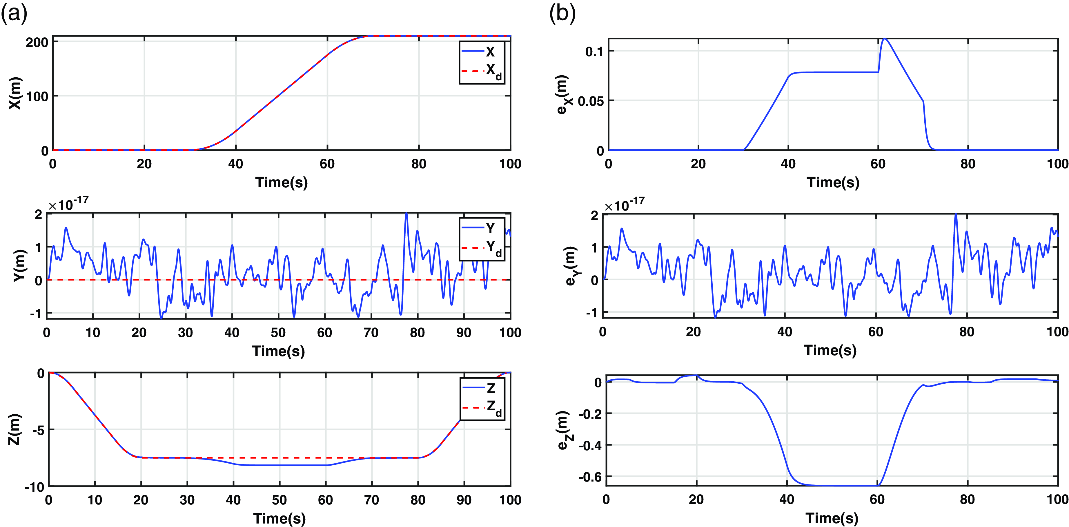
Figure 14. Second scenario results: (a) desired and actual horizontal positions and altitude; (b) corresponding tracking errors.
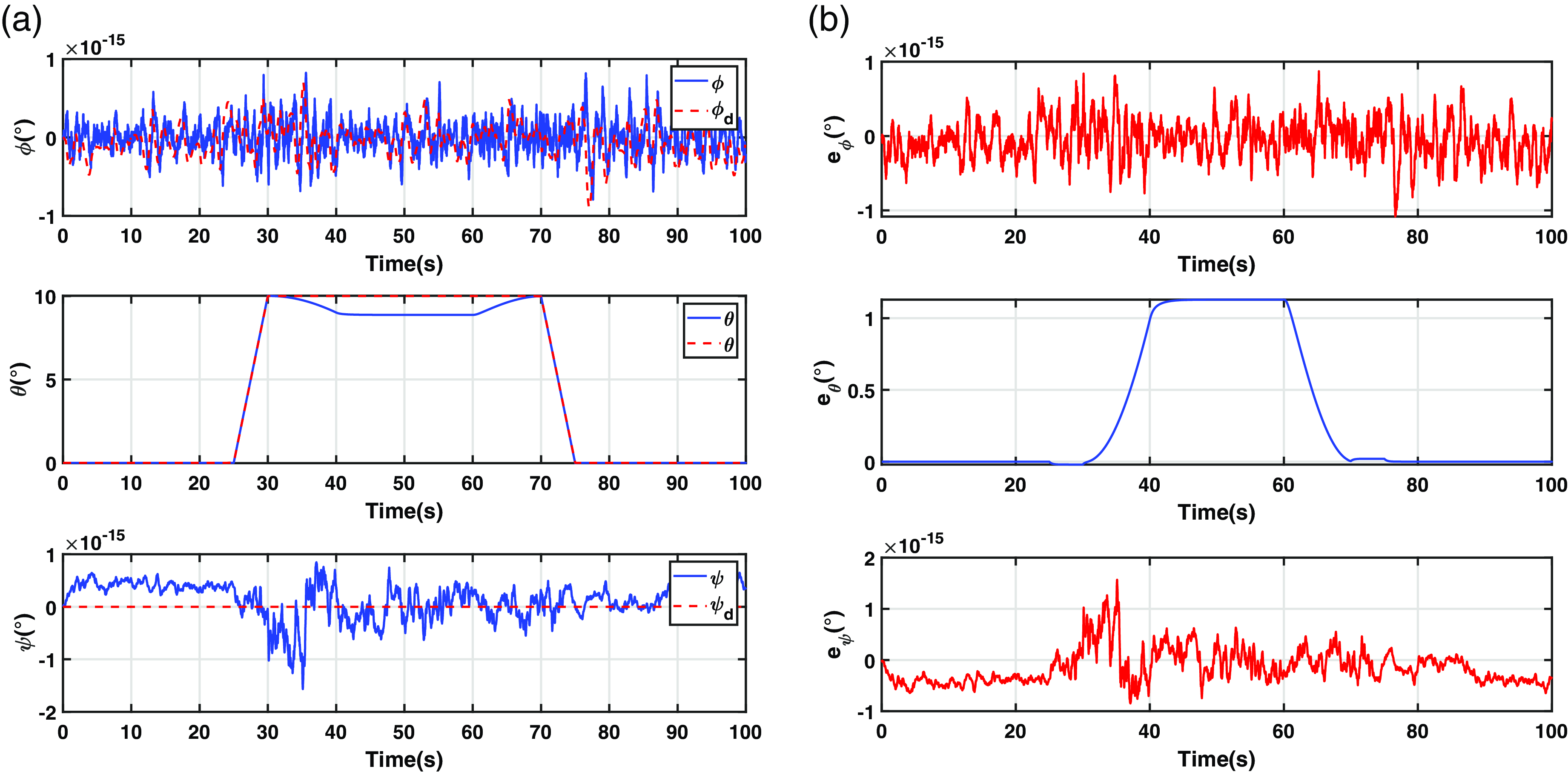
Figure 15. Second scenario results: (a) desired and actual attitude of the CSF-TRUAV; (b) from top to bottom roll, pitch and heading tracking errors ${e_\psi }$
.
${e_\psi }$
.
Figure 13 depicts the 3D reference path and the path followed by the drone. The external disturbances, caused by the neglected aerodynamic forces and moments, led to a remarkable discrepancy between the two variables.
Figure 14(a) plots in more detail the temporal variation of the two trajectories, while Fig. 14(b) is a plot of the corresponding tracking errors. As the figure shows, the suppression of the feed-forward terms from the control equations has little effect on the tracking errors in the forward and lateral positions. When it comes to the altitude, however, the effect of this action is noticeable. It leads to steady-state errors in both variables when the drone enters cruise flight, i.e., when the aerodynamic forces and moments start building up.
Figure 15(a) depicts the control performances in terms of attitude control. The corresponding tracking errors are presented in Fig. 15(b). The neglected aerodynamic moments did not affect the yaw and roll angles control. Their effect on the pitch angle, on the other hand, was remarkable, especially during the cruise phase, for the same reasons regarding position control.
It is important to note that the error observed in the pitch angle response has an indirect effect on the forward position of the drone. In fact, the dynamics of the forward position depend on the pitch angle (Equation (35)). The nonlinear nature of the backstepping controller, however, allows it to take into account any change in the pitch angle instantly.
Figure 16(a) presents the control efforts for the second scenario, while Fig. 16(b) plots the tilt angle and airspeed. The control efforts have similar behaviour in comparison to the first scenario, with a slight difference in the cruise flight phase. The evolution of the tilt angle is also slightly different in this scenario, despite the forward position being unaffected by the suppression of the feed-forward terms. This is due to the coupling between the z-axis controller and that of the forward position. Any decrease in the control efforts of the front rotors is compensated for by an increase in the tilt angle.
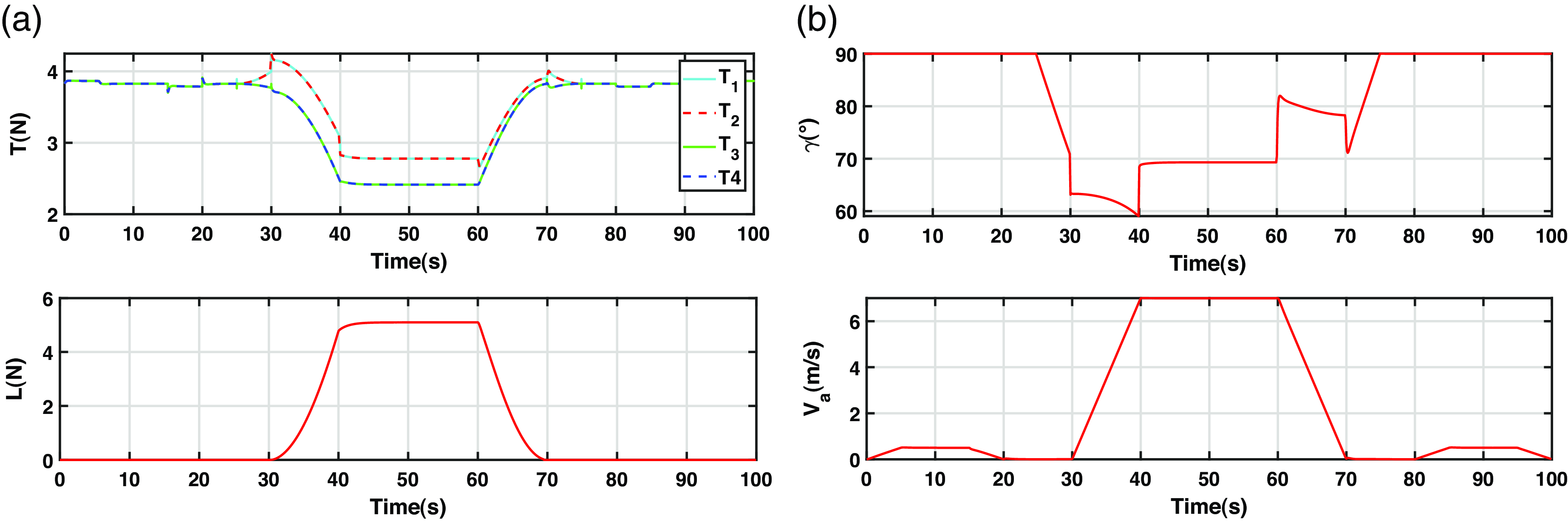
Figure 16. Results of the second scenario: (a) thrust and lift forces; (b) tilt angle and airspeed.
5.3 Third scenario: Implicit compensation of aerodynamic forces and moments through integral-backstepping control
In this section, the effects of the aerodynamic forces and moments are compensated without explicit estimation. This is achieved through the design of a robust, integral backstepping controller. For the sake of brevity, only the design steps for the roll angle are detailed. The same steps are followed for the remaining variables.
Let us consider the variable ${\phi _0}$
, such that
${\phi _0}$
, such that
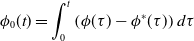 \begin{align} \phi_0 (t)=\int_0^t\left(\phi(\tau)-\phi^*(\tau)\right) d \tau \end{align}
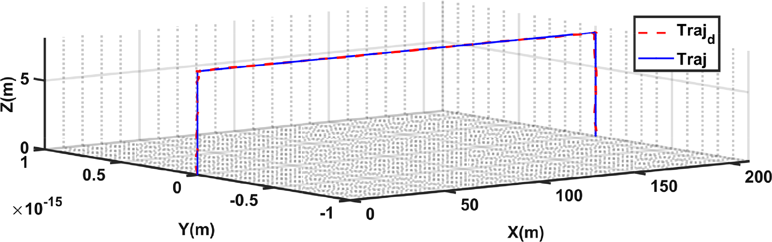
Figure 17. Third scenario results: 3D path followed by the CSF-TRUAV.
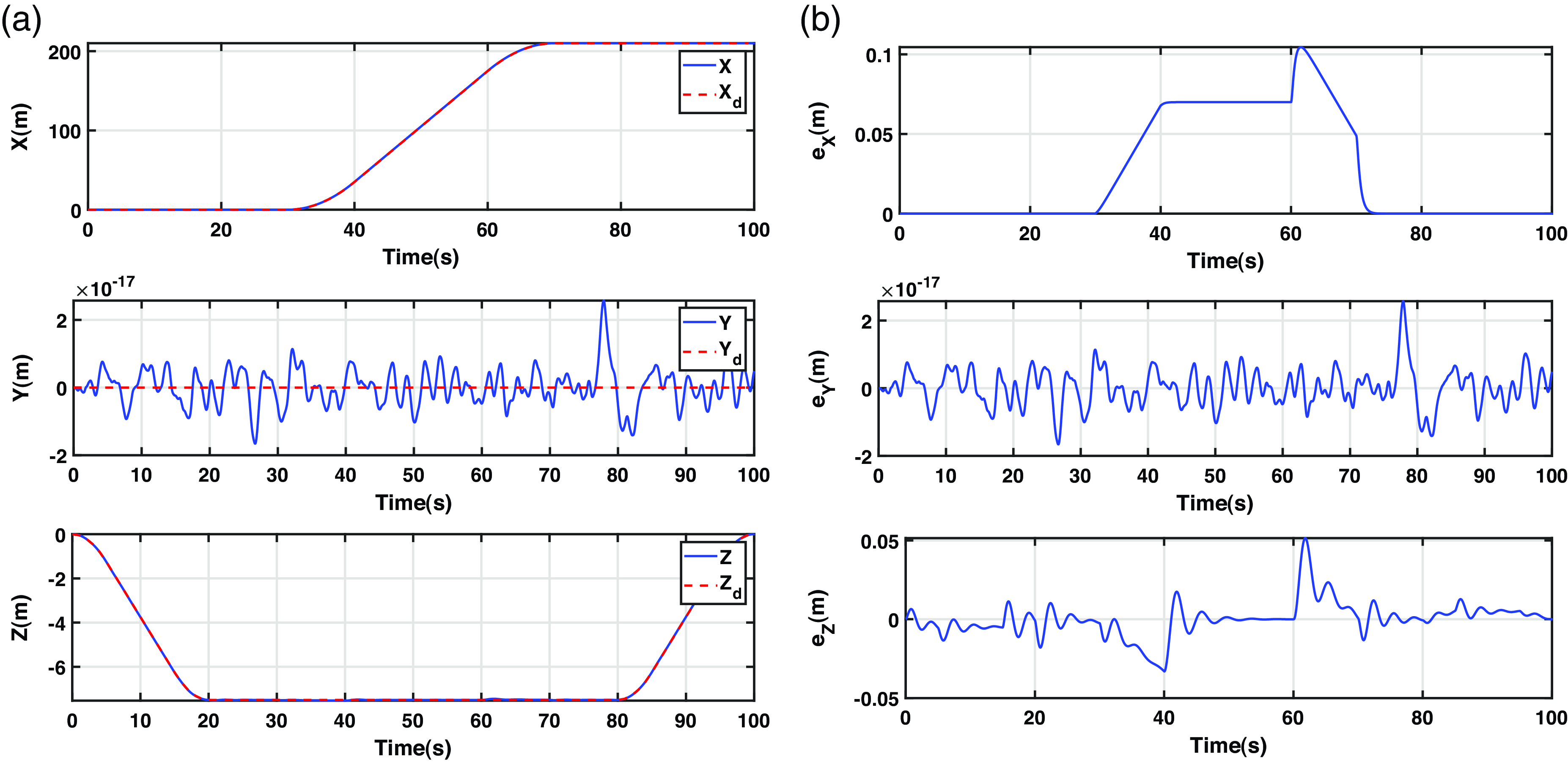
Figure 18. Third scenario results: (a) desired and actual horizontal positions and altitude; (b) corresponding tracking errors.
The virtual control input ${\dot \phi _d}$
in Equation (62) is modified to take into account the integral of the tracking error
${\dot \phi _d}$
in Equation (62) is modified to take into account the integral of the tracking error
 \begin{align}{\dot \phi _d} = {\dot \phi ^{\rm{*}}} - {\alpha _{{\phi _1}}}{\phi _1} - {\lambda _\phi }{\phi _0}{\rm{\;\;\;\;}}{\alpha _{{\phi _1}}} \gt 0,\;\;\;\;{\lambda _\phi } \gt 0\end{align}
Let us define a new tracking error ${\phi _2}$
, such that
${\phi _2}$
, such that
 \begin{align}{\phi _2} = \dot \phi - {\dot \phi _d} = \dot \phi - {\dot \phi ^{\rm{*}}} + {\alpha _{{\phi _1}}}{\phi _1} + {\lambda _\phi }{\phi _0}\end{align}
To minimise the tracking error ${\phi _2}$
, the following Lyapunov function is considered
${\phi _2}$
, the following Lyapunov function is considered
 \begin{align} V_2 = \frac{1}{2}\phi _2^2\end{align}
The time derivative of ${V_2}$
 \begin{align}{\dot V_2} = {\phi _2}{\dot \phi _2}\end{align}
 \begin{align} = {\phi _2}\left( {\dot \theta \dot \psi {a_1} + {b_1}{\tau _\phi } + {b_1}l - {{\ddot \phi }^{\rm{*}}} + {\alpha _{{\phi _1}}}{\phi _2} + \left( {{\lambda _\phi } - \alpha _{{\phi _1}}^2} \right){\phi _1} - {\alpha _{{\phi _1}}}{\lambda _\phi }{\phi _0}} \right)\end{align}
To guarantee asymptotic stability, the reference for the roll torque ${\tau _\phi }$
is calculated as
${\tau _\phi }$
is calculated as
 \begin{align}{\tau _\phi } = \frac{1}{{{b_1}}}\left( { - {a_1}\dot \theta \dot \psi + {{\ddot \phi }^{\rm{*}}} - \left( {{\alpha _{{\phi _1}}} + {\alpha _{{\phi _2}}}} \right){\phi _2} - \left( {{\lambda _\phi } - \alpha _{{\phi _1}}^2} \right){\phi _1} + {\alpha _{{\phi _1}}}{\lambda _\phi }{\phi _0}} \right)\end{align}
Figure 19. Third scenario results: (a) desired and actual attitude of the CSF-TRUAV; (b) from top to bottom roll, pitch and heading tracking errors.
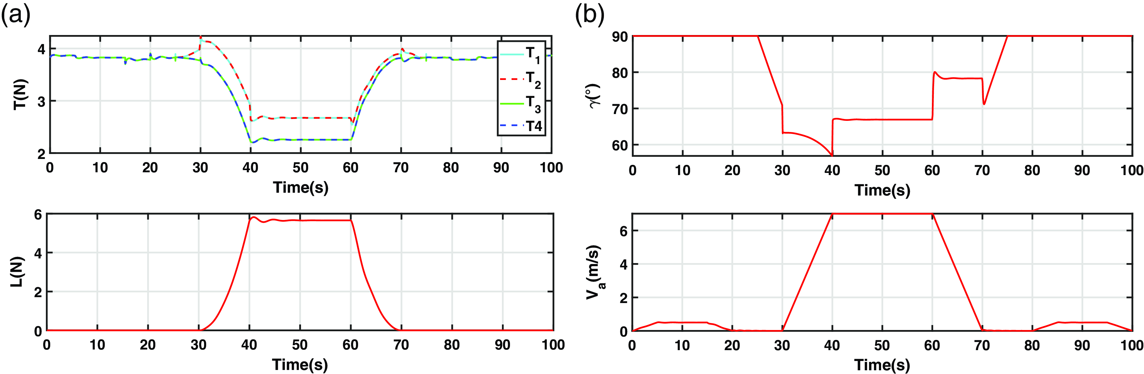
Figure 20. Results of the third scenario: (a) thrust and lift forces; (b) tilt angle and airspeed.
The tracking errors associated to the remaining variables are
 \begin{align*}{\theta _1} = \theta - {\theta ^{\rm{*}}}\quad {\theta _2} = \dot \theta - {\dot \theta ^{\rm{*}}} + {\alpha _{{\theta _1}}}{\theta _1} + {\lambda _\theta }{\theta _0}\end{align*}
 \begin{align*}{\psi _1} = \psi - {\psi ^{\rm{*}}}\quad {\psi _2} = \dot \psi - {\dot \psi ^{\rm{*}}} + {\alpha _{{\psi _1}}}{\psi _1} + {\lambda _\psi }{\psi _0}\end{align*}
 \begin{align*}{z_1} = z - {z^{\rm{*}}}\quad {z_2} = \dot z - {\dot z^{\rm{*}}} + {\alpha _{{z_1}}}{z_1} + {\lambda _z}{z_0}\end{align*}
 \begin{align*}{x_1} = x - {x^{\rm{*}}}\quad {x_2} = \dot x - {\dot x^{\rm{*}}} + {\alpha _{{x_1}}}{x_1} + {\lambda _x}{x_0}\end{align*}
 \begin{align*}{y_1} = y - {y^{\rm{*}}}\quad {y_2} = \dot y - {\dot y^{\rm{*}}} + {\alpha _{{y_1}}}{y_1} + {\lambda _y}{y_0}\end{align*}
Following the same steps as for the design of the backstepping controller of the roll angle, the control equations of the remaining variables are
 \begin{align}{\tau _\theta } = \frac{1}{{{b_2}}}\left( { - {a_2}\dot \phi \dot \psi + {{\ddot \theta }^{\rm{*}}} - \left( {{\alpha _{{\theta _1}}} + {\alpha _{{\theta _2}}}} \right){\theta _2} - \left( {{\lambda _\theta } - \alpha _{{\theta _1}}^2} \right){\theta _1} + {\alpha _{{\theta _1}}}{\lambda _\theta }{\theta _0}} \right)\end{align}
 \begin{align}{\tau _\psi } = \frac{1}{{{b_3}}}\left( { - {a_3}\dot \phi \dot \theta + {{\ddot \psi }^{\rm{*}}} - \left( {{\alpha _{{\psi _1}}} + {\alpha _{{\psi _2}}}} \right){\psi _2} - \left( {{\lambda _\psi } - \alpha _{{\psi _1}}^2} \right){\psi _1} + {\alpha _{{\phi _1}}}{\lambda _\psi }{\psi _0}} \right)\end{align}
 \begin{align}{U_z} = m\left( { - g + {{\ddot z}^{\rm{*}}} - \left( {{\alpha _{{z_1}}} + {\alpha _{{z_2}}}} \right){z_2} - \left( {{\lambda _z} - \alpha _{{z_1}}^2} \right){z_1} + {\alpha _{{z_1}}}{\lambda _z}{z_0}} \right)\end{align}
 \begin{align}{u_x} = m\left( {{{\ddot x}^{\rm{*}}} - \left( {{\alpha _{{x_1}}} + {\alpha _{{x_2}}}} \right){x_2} - \left( {{\lambda _x} - \alpha _{{x_1}}^2} \right){x_1} + {\alpha _{{x_1}}}{\lambda _x}{x_0}} \right)\end{align}
 \begin{align}{u_y} = m\left( {{{\ddot y}^{\rm{*}}} - \left( {{\alpha _{{y_1}}} + {\alpha _{{y_2}}}} \right){y_2} - \left( {{\lambda _y} - \alpha _{{y_1}}^2} \right){y_1} + {\alpha _{{y_1}}}{\lambda _y}{y_0}} \right)\end{align}
Figure 17 depicts the path followed by the drone when controlled by the designed integral backstepping controllers. These results are very close to those of the first scenario, where the aerodynamic forces and moments were explicitly taken into account in the control equations.
Figure 18(a) illustrates in more detail the effect of the integral action on the trajectory tracking performances. As illustrated by Fig. 18(b), the inclusion of the integral action allowed the cancellation of the errors caused by the perturbation resulting from the aerodynamic forces and moments. This leads to more accurate trajectory tracking compared to the second scenario.
The attitude-tracking results of the third scenario are illustrated in Fig. 19(a). As Fig. 19(b) shows, the tracking errors of the roll and yaw angles are negligible as was the case in the first and second scenarios. The pitch errors, on the other hand, are highly reduced in comparison to the second scenario and slightly higher than that of the first scenario. Another advantage of the feed-forward compensation of the aerodynamic perturbations is its instantaneous effect. As can be observed when comparing Figs. 19(b)–11(b), the implicit compensation results in a higher response time compared to the first scenario.
Figure 20(a) plots the evolution of the control efforts and Fig. 20(b) corresponds to the tilt angle generated by the integral-backstepping controller. These results are very close to those observed in the first scenario, with a slight increase in the overshoots observed at the beginning of the forward and backward transitions.
Table 2 summarises the average thrust force of the four actuators and the average tilt angle during the cruise flight phase. The control efforts generated by the integral backstepping controller are very close to those generated by the control with feed-forward compensation of aerodynamic perturbations.
Table 2. Average thrust forces and tilt angle during the cruise flight phase
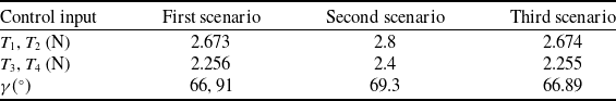
6.0 Conclusion
This paper presented a new design for a tilt-rotor convertible UAV that combines the high cruising speed and endurance of fixed-wing drones with the hovering and vertical takeoff and landing capabilities of multi-rotors. This design, which we termed CSF-TRUAV, does not contain any control surfaces. Such a characteristic not only facilitates its construction but also enhances its reliability.
The CSF-TRUAV is actuated using only propellers in both VTOL and fixed-wing modes. To accommodate this particularity, a new control strategy was proposed. Unlike previous works, which use a separate controller for each flight phase, the proposed solution employs a single controller for the whole flight envelope.
Simulation results, conducted on the full nonlinear model of the famous Zagi flying wing drone, showed the ineffectiveness of a classical backstepping controller. In fact, unless the aerodynamic forces and moments are taken into account in the control equations, steady-state errors are observed during the cruise flight phase. To solve this issue, an integral backstepping controller was considered. This allowed for the cancellation of the effect of the aerodynamic forces and moments without the need for an explicit estimation of their magnitudes.
Future works will target the construction of a prototype of the proposed concept and the implementation of the proposed control strategy. A quantitative evaluation of the aerodynamic and energetic performances of the proposed design and the associated controller is also an interesting future work direction.
Competing interests
The authors declare none.


