


Introduction
Systematic paleontology is essential work in paleontology and biostratigraphy, because it helps reveal biological evolution in deep time. Despite the accurate taxonomic identification of fossils being essential for research, traditional methods rely only on individual identification, which is time-consuming, labor-intensive, and subjective. Alternatively, machine learning can help experts identify biological specimens and significantly increase efficiency (MacLeod et al. Reference MacLeod, Benfield and Culverhouse2010), as was intended since it was first proposed 50 years ago (Pankhurst Reference Pankhurst1974). Traditional machine learning methods rely on a set of characteristics (e.g., geometric features) selected or designed manually by experts. Analytical methods can benefit from the use of machine learning methods, such as shallow artificial neural networks, support vector machines, decision trees, clustering, and naive Bayes classifiers, to handle nonlinear complex tasks (MacLeod Reference MacLeod2007), achieving a suitable efficiency on small datasets. Owing to the development of computer science and the advent of big data, deep learning has advanced substantially over the past decade (LeCun et al. Reference LeCun, Bengio and Hinton2015), enabling the analysis of massive, high-dimensional, and complex data (Hinton and Salakhutdinov Reference Hinton and Salakhutdinov2006). Remarkably, in the field of computer vision, deep convolutional neural networks (DCNNs) (Krizhevsky et al. Reference Krizhevsky, Sutskever and Hinton2012; Szegedy et al. Reference Szegedy, Liu, Jia, Sermanet, Reed, Anguelov, Erhan, Vanhoucke and Rabinovich2015) can learn and automatically extract features from images. In the past few years, convolutional neural networks (CNNs) have been increasingly applied in geoscience and its multidisciplinary fields, as reported in the Web of Science (Fig. 1). Meanwhile, previous studies have proven the feasibility of using deep learning methods for the automatic identification of biotics or fossils (MacLeod et al. Reference MacLeod, Benfield and Culverhouse2010; Romero et al. Reference Romero, Kong, Fowlkes, Jaramillo, Urban, Oboh-Ikuenobe, D'Apolito and Punyasena2020).

Figure 1. Statistics of publications and citations of the topics of machine learning (ML) and convolutional neural networks (CNNs) in geoscience and its multidisciplinary fields from Web of Science (to 13 August 2021).
Recent automatic identification methods in taxonomic research using deep learning have mainly focused on modern organisms, with only a few considering fossils (mainly microfossils), including foraminifera (Zhong et al. Reference Zhong, Ge, Kanakiya, Marchitto and Lobaton2017; Hsiang et al. Reference Hsiang, Brombacher, Rillo, Mleneck-Vautravers, Conn, Lordsmith, Jentzen, Henehan, Metcalfe and Fenton2019; Mitra et al. Reference Mitra, Marchitto, Ge, Zhong, Kanakiya, Cook, Fehrenbacher, Ortiz, Tripati and Lobaton2019; Carvalho et al. Reference Carvalho, Fauth, Fauth, Krahl, Moreira, Fernandes and Von Wangenheim2020; Marchant et al. Reference Marchant, Tetard, Pratiwi, Adebayo and de Garidel-Thoron2020; Pires de Lima et al. Reference Pires de Lima, Welch, Barrick, Marfurt, Burkhalter, Cassel and Soreghan2020), radiolarians (Keçeli et al. Reference Keçeli, Kaya and Keçeli2017, Reference Keçeli, Keçeli and Kaya2018; Tetard et al. Reference Tetard, Marchant, Cortese, Gally, de Garidel-Thoron and Beaufort2020), planktonic life forms (Al-Barazanchi et al. Reference Al-Barazanchi, Verma and Wang2015, Reference Al-Barazanchi, Verma and Wang2018; Li and Cui Reference Li and Cui2016), coccoliths (Beaufort and Dollfus Reference Beaufort and Dollfus2004), diatoms (Urbankova et al. Reference Urbankova, Scharfen and Kulichová2016; Bueno et al. Reference Bueno, Deniz, Pedraza, Ruiz-Santaquiteria, Salido, Cristóbal, Borrego-Ramos and Blanco2017; Pedraza et al. Reference Pedraza, Bueno, Deniz, Cristóbal, Blanco and Borrego-Ramos2017; Kloster et al. Reference Kloster, Langenkämper, Zurowietz, Beszteri and Nattkemper2020; Lambert and Green Reference Lambert and Green2020), pollen grains (Marcos et al. Reference Marcos, Nava, Cristóbal, Redondo, Escalante-Ramírez, Bueno, Déniz, González-Porto, Pardo and Chung2015; Kong et al. Reference Kong, Punyasena and Fowlkes2016; Sevillano and Aznarte Reference Sevillano and Aznarte2018; Bourel et al. Reference Bourel, Marchant, de Garidel-Thoron, Tetard, Barboni, Gally and Beaufort2020; Romero et al. Reference Romero, Kong, Fowlkes, Jaramillo, Urban, Oboh-Ikuenobe, D'Apolito and Punyasena2020), plants (Liu et al. Reference Liu, Zhang, He and Li2018a; Kaya et al. Reference Kaya, Keceli, Catal, Yalic, Temucin and Tekinerdogan2019; Too et al. Reference Too, Yujian, Njuki and Yingchun2019; Ngugi et al. Reference Ngugi, Abelwahab and Abo-Zahhad2021), wild mammals (Villa et al. Reference Villa, Salazar and Vargas2017; Norouzzadeh et al. Reference Norouzzadeh, Nguyen, Kosmala, Swanson, Palmer, Packer and Clune2018; Tabak et al. Reference Tabak, Norouzzadeh, Wolfson, Sweeney, VerCauteren, Snow, Halseth, Di Salvo, Lewis and White2019), insects (Rodner et al. Reference Rodner, Simon, Brehm, Pietsch, Wägele and Denzler2015; Martineau et al. Reference Martineau, Conte, Raveaux, Arnault, Munier and Venturini2017; Valan et al. Reference Valan, Makonyi, Maki, Vondráček and Ronquist2019), and bones and teeth (Domínguez-Rodrigo and Baquedano Reference Domínguez-Rodrigo and Baquedano2018; Byeon et al. Reference Byeon, Domínguez-Rodrigo, Arampatzis, Baquedano, Yravedra, Maté-González and Koumoutsakos2019; Hou et al. Reference Hou, Cui, Canul-Ku, Jin, Hasimoto-Beltran, Guo and Zhu2020; MacLeod and Kolska Horwitz Reference MacLeod and Kolska Horwitz2020). However, various drawbacks remain to be addressed. First, most existing studies have focused on species-level automatic identification, but such a method can only be applied to a few common taxa in a specific clade. Hsiang et al. (Reference Hsiang, Brombacher, Rillo, Mleneck-Vautravers, Conn, Lordsmith, Jentzen, Henehan, Metcalfe and Fenton2019) collected the largest planktonic foraminifera dataset, containing 34,000 images from 35 species (comprising most living planktonic foraminifera). They combined the efforts of more than 20 taxonomic experts to generate a rich and accurate dataset for deep learning. However, other fossil clades, such as benthic foraminifera, usually contain thousands of species, but recent studies only analyzed a limited number of taxa (Pires de Lima et al. Reference Pires de Lima, Welch, Barrick, Marfurt, Burkhalter, Cassel and Soreghan2020). Consequently, few experts can truly benefit from such studies. Second, although previous research provides publicly available codes and models, taxonomists may face usage difficulties owing to software limitations. Thus, providing an end-to-end framework is necessary and critical for the adoption of deep learning models. Third, experiments were conducted based on a dataset collected from personal collections (Mitra et al. Reference Mitra, Marchitto, Ge, Zhong, Kanakiya, Cook, Fehrenbacher, Ortiz, Tripati and Lobaton2019), research institution collections (Hsiang et al. Reference Hsiang, Brombacher, Rillo, Mleneck-Vautravers, Conn, Lordsmith, Jentzen, Henehan, Metcalfe and Fenton2019), public literature, and multiple sources (Liu and Song Reference Liu and Song2020; Pires de Lima et al. Reference Pires de Lima, Welch, Barrick, Marfurt, Burkhalter, Cassel and Soreghan2020). Although collecting data from various sources can partially compensate for data scarcity, tens of thousands or even millions of samples are usually needed to develop successful deep learning applications (Deng et al. Reference Deng, Dong, Socher, Li, Li and Li2009). Traditional data collection is unsuitable for constructing massive datasets unless geologists can standardize or digitize unstructured data scattered in paper records and personal hard disks (Wang et al. Reference Wang, Hazen, Cheng, Stephenson, Zhou, Fox, Shen, Oberhänsli, Hou, Ma, Feng, Fan, Ma, Hu, Luo, Wang and Schiffries2021).
To improve data collection, we used web crawlers to collect the largest Fossil Image Dataset (FID) currently available from the Internet, obtaining more than 415,000 images. We then leveraged the high performance of DCNNs to perform the automatic taxonomic identification of fossils. Rather than focusing on a particular fossil group, we first aimed to identify fossil clades. This approach can support research in the geosciences and help disseminate paleontological knowledge to the public. We also deployed the resulting model on a server for public access at www.ai-fossil.com.
Data and Methods
Data
We collected the FID from the public Internet using web crawlers and then we manually checked the images and their corresponding labels. The uniform resource locators (URLs) of the images highlighted in this study are listed in Supplementary Table S1, and those of all the images in the FID are available at https://doi.org/10.5281/zenodo.6333970. Some collected images showed a large area of unnecessary backgrounds, which we manually cropped to preserve the fossiliferous regions only. Data on conodont, foraminifera, and trace fossils were supplemented from the literature, using the method demonstrated in Liu and Song (Reference Liu and Song2020). We collected 415,339 images belonging to 50 clades in the FID (Fig. 2). The 50 clades consist of five superclades: (1) invertebrates: ammonoids, belemnites, bivalves, blastoids, brachiopods, bryozoans, chelicerates, corals, crinoids, crustaceans, echinoids, gastropods, graptolites, insects, myriapods, nautiloids, ophiuroids, sponges, starfish, stromatolites, and trilobites; (2) vertebrates: agnatha, amphibians, avialae, bone fragments, chondrichthyes, crocodylomorphs, mammals, mammalian teeth, marine reptiles, ornithischians, osteichthyes, placoderms, pterosaurs, reptilian teeth, sauropodomorphs, shark teeth, snakes, theropods, and turtles; (3) plants: angiosperms, gymnosperms, petrified wood, and pteridophytes; (4) microfossils: conodonts, foraminifera, ostracods, radiolarians, and spores or pollen; and (5) trace fossils.
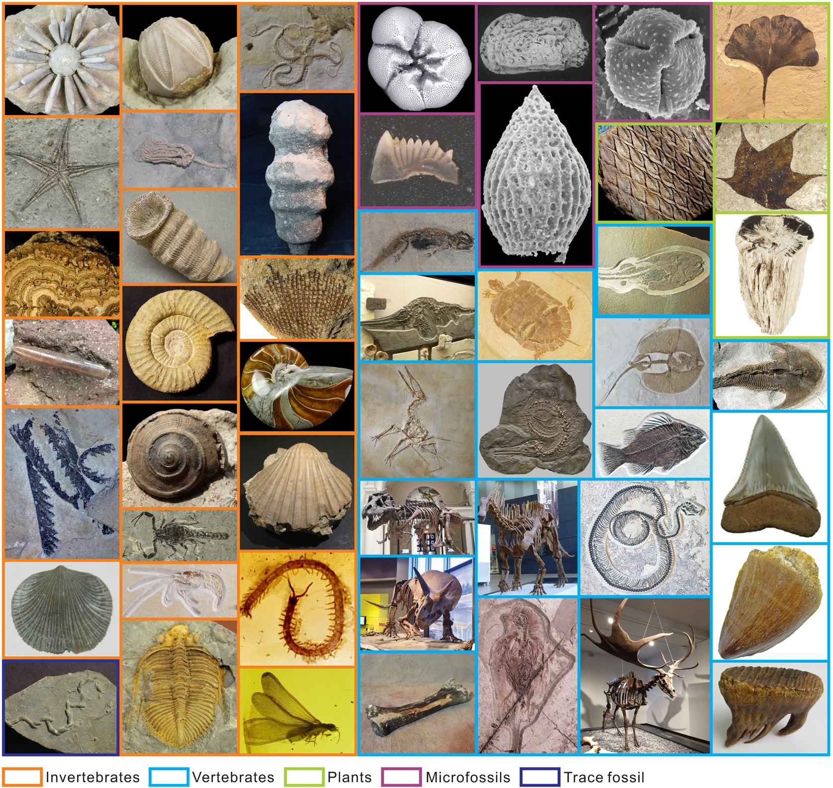
Figure 2. Example images of each class in our dataset, which contains 50 clades (Table 1). Specimens are not to scale. The source URLs of the images are provided in Supplementary Table S1.
Table 1. Number of samples for the three subsets and each class.

Web Crawlers
Web crawlers have been used to collect data from open web pages for data mining (Helfenstein and Tammela Reference Helfenstein and Tammela2017; Lopez-Aparicio et al. Reference Lopez-Aparicio, Grythe, Vogt, Pierce and Vallejo2018) and deep learning (Xiao et al. Reference Xiao, Xia, Yang, Huang and Wang2015). A web crawler is a programmed script or software that browses web pages systematically and automatically to retrieve specific information (Kausar et al. Reference Kausar, Dhaka and Singh2013) by sending requests for documents on servers to resemble a normal request. The script examines the returned data per web page to select useful information, such as image URLs in this study. We used search engines (e.g., Google and Bing) to collect fossil images by searching for keywords (e.g., “trilobite”) and then downloaded the images and their associated URLs to a local storage site. We examined different keywords to download fossil images from different geological ages and regions. In addition, we removed duplicate images by applying algorithms such as AntiDupl.NET.
Computing Environments
All analysis codes were executed on a Dell Precision 7920 Workstation running Microsoft Windows 10 Professional. The workstation was equipped with two Intel Xeon Silver 4216 processors, 128 GB of memory, and two NVIDIA GeForce GTX 2080Ti graphics processors (11 GB of memory per graphics processor). To implement the deep learning framework, we used TensorFlow v. 1.13.1 (Abadi et al. Reference Abadi, Barham, Chen, Chen, Davis, Dean, Devin, Ghemawat, Irving and Isard2016) and Keras v. 2.2.4 (with TensorFlow backend; Chollet Reference Chollet2015) in Python v. 3.6.5. The required preinstalled Python libraries, algorithms for analysis, and model weights are available at https://github.com/XiaokangLiuCUG/Fossil_Image_Dataset. All the images used and their URLs are uploaded at https://doi.org/10.5281/zenodo.6333970.
Convolutional Neural Network
A CNN is a supervised learning algorithm that requires images to be input with their corresponding labels for training. CNNs can handle image-based tasks, including image recognition (LeCun et al. Reference LeCun, Bottou, Bengio and Haffner1998), object detection (Redmon et al. Reference Redmon, Divvala, Girshick and Farhadi2016), facial detection (Li et al. Reference Li, Lin, Shen, Brandt and Hua2015), semantic segmentation (Long et al. Reference Long, Shelhamer and Darrell2015), and image retrieval (Babenko et al. Reference Babenko, Slesarev, Chigorin and Lempitsky2014). Fukushima (Reference Fukushima1980) proposed a self-organized artificial neural network called the neocognitron, a predecessor of CNNs, that tolerates image shifting and deformation based on the work by Hubel and Wiesel (Reference Hubel and Wiesel1962). LeCun et al. (Reference LeCun, Bottou, Bengio and Haffner1998) first used a backpropagation method in LeNet-5 to learn the convolution kernel coefficients directly from MNIST (Mixed National Institute of Standards and Technology database, which contains 60,000 grayscale images of handwritten digits) images. Subsequently, DCNNs were created, which usually contain dozens or even hundreds of hidden layers, such as VGG-16 (Simonyan and Zisserman Reference Simonyan and Zisserman2014), GoogLeNet (Szegedy et al. Reference Szegedy, Liu, Jia, Sermanet, Reed, Anguelov, Erhan, Vanhoucke and Rabinovich2015), ResNet (He et al. Reference He, Zhang, Ren and Sun2016), Inception-ResNet (Szegedy et al. Reference Szegedy, Ioffe, Vanhoucke and Alemi2017), and PNASNet (Liu et al. Reference Liu, Zoph, Neumann, Shlens, Hua, Li, Fei-Fei, Yuille, Huang and Murphy2018b), and DCNNs are widely used in many domains.
Inputs are the pixel matrix of an image, which is usually represented by a grayscale channel or red-green-blue channels for 2D images (e.g., trilobite image in Fig. 3), and its corresponding label. In general, a conventional CNN mainly consists of convolutional layers, pooling layers, a fully connected layer, and an output layer (Krizhevsky et al. Reference Krizhevsky, Sutskever and Hinton2012). An input image is successively convolved with learned filters in each layer, where each activation map can also be interpreted as a feature map. Then a nonlinear activation function performs a transformation to learn complex decision boundaries across images. The pooling layers are used for downsampling, considering that adjacent pixels contain similar information. Convolutional and pooling layers are usually combined and reused multiple times for feature extraction (Fig. 3). Then, the fully connected layer combines thousands of feature maps for the final classification. The output layer uses the softmax function in TensorFlow to generate a probability vector to represent the classification result. Cross-entropy is usually used as the objective function for measuring errors from predicted and true labels (Botev et al. Reference Botev, Kroese, Rubinstein, L'Ecuyer, Rao and Govindaraju2013). The backpropagation of the gradient method was conducted to minimize the cross-entropy value and maximize the classification performance of the architecture (Rumelhart et al. Reference Rumelhart, Hinton and Williams1986).

Figure 3. Schematic of a convolutional neural network, modified from Krizhevsky et al. (Reference Krizhevsky, Sutskever and Hinton2012). FC layer, fully connected layer.
DCNNs contain massive parameters, and they should be trained on large datasets such as ImageNet (https://image-net.org; Deng et al. Reference Deng, Dong, Socher, Li, Li and Li2009), which contains more than 1.2 million labeled images from 1000 classes. Alternatively, transfer learning can be used for small training datasets (Tan et al. Reference Tan, Sun, Kong, Zhang, Yang and Liu2018; Brodzicki et al. Reference Brodzicki, Piekarski, Kucharski, Jaworek-Korjakowska and Gorgon2020; Koeshidayatullah et al. Reference Koeshidayatullah, Morsilli, Lehrmann, Al-Ramadan and Payne2020). In transfer learning, instead of training a CNN architecture from randomly initialized parameters, the parameters are obtained from pretraining on other recognition tasks with a large dataset for initialization. Thus, transfer learning can reduce computing costs, improve feature extraction, and accelerate the training convergence of the model. Transfer learning methods mainly include feature extraction and fine-tuning. For feature extraction, convolutional layers are frozen so that the parameters are not updated during training. In this study, we froze the shallow layers (half the network layers) to only train the deep layers. We also evaluated fine-tuning, in which pretrained parameters are used as initialization, and training was applied to all the network parameters with a small learning rate.
To increase the model's performance and the generalization ability of the evaluated DCNNs, we used data augmentation (Wang and Perez Reference Wang and Perez2017), randomly adding noise to enhance the robustness of the algorithm against the contrast ratio, color space, and brightness, which are not the main identification characteristics of classes in fossil images (Shorten and Khoshgoftaar Reference Shorten and Khoshgoftaar2019). In addition, we applied random cropping, rotating, and resizing of the images using preprocessing packages in TensorFlow (Abadi et al. Reference Abadi, Barham, Chen, Chen, Davis, Dean, Devin, Ghemawat, Irving and Isard2016) and Keras (Chollet Reference Chollet2015). Data augmentation allows expansion of the training set and partially mitigates overfitting (Wang and Perez Reference Wang and Perez2017). In this study, we examined different combinations of data augmentation operations. We used the downscaled image for inference to reduce the image preprocessing time. The width and height of all the images were limited to 512 and then used to create TFRecord files.
Training
We randomly split the collected FID into three subsets, as detailed in Table 1. The training set was used for determining the model parameters, while the validation set was used to adjust the hyperparameters (untrainable parameters) of the model and verify the performance during training, and the test set was used to evaluate the generalization ability of the final model. To test the influence of data volume on individual class accuracy, we also trained on a reduced FID, in which each class contained 1200 training images, and tested the final performance on the same test set. We used the top-1 accuracy (the true class matches the predicted label with the biggest possibility) and top-3 accuracy (the true class matches the predicted label for any of the three most probable classes) to measure the performance of the DCNN architectures. We evaluated three conventional DCNNs, namely Inception-v4 (Szegedy et al. Reference Szegedy, Ioffe, Vanhoucke and Alemi2017), Inception-ResNet-v2 (Szegedy et al. Reference Szegedy, Ioffe, Vanhoucke and Alemi2017), and PNASNet-5-large (Liu et al. Reference Liu, Zoph, Neumann, Shlens, Hua, Li, Fei-Fei, Yuille, Huang and Murphy2018b), which have achieved excellent results on ImageNet. We ran 14 trials to optimize the performance of the models with different hyperparameter sets. In addition, we considered transfer learning and training from randomly initialized parameters. For transfer learning, we fine-tuned all trainable layers and froze the shallow layers (half of the DCNN layers) to only train the remaining layers, as detailed in Table 2. During training, the algorithm randomly fed a batch of images per iteration (step). An epoch was complete when all training images were fed to the architecture once, noting that dozens of epochs are usually required for the model convergence. The output logs can facilitate optimization. The test set was used to determine the ultimate performance of each DCNN. The main experiments were performed using Inception-v4 to optimize the hyperparameters, and then we trained on the other two architectures. We did not try all possible experiments to optimize the hyperparameters, because we evaluated the identification of biotic and abiotic grains in thin sections in the experiment by Liu and Song (Reference Liu and Song2020). Instead, we used the main settings and tried to optimize several critical hyperparameters, such as those for transfer learning, fine-tuning, learning rate, and data augmentation operations.
Table 2. Experiments for the three deep convolutional neural network (DCNN) architectures. For the “Load weights” column, pre-trained parameters were used for variable initialization (i.e., transfer learning). In the “Train layers” column, the settings of training/froze layers for Inception-v4 and Inception-ResNet-v2 follow the methods of Liu and Song (Reference Liu and Song2020). For PNASNet-5-large, the trainable layers include cell_6, cell_7, cell_8, cell_9, cell_10, cell_11, aux_7, and final_layer in Liu et al. (Reference Liu, Zoph, Neumann, Shlens, Hua, Li, Fei-Fei, Yuille, Huang and Murphy2018b). “DA with RC” shows data augmentation with the random crop, the random cropped image covers 0.4–1 range of the original image (except experiment 7, which used a range of 0.65–1). Other data augmentation methods follow the methods of Szegedy et al. (Reference Szegedy, Ioffe, Vanhoucke and Alemi2017) and Liu et al. (Reference Liu, Zoph, Neumann, Shlens, Hua, Li, Fei-Fei, Yuille, Huang and Murphy2018b). All experiments used batch normalization, dropout (with 0.8), and Adam optimizer. The input size of Inception-v4 and Inception-ResNet-v2 is 299 × 299, and that of PNASNet-5-large is 331 × 331. The decay rate for experiment 6 is 0.96 when training epochs <15 and 0.9 when training epochs ≥15. Experiment 13 was trained on the reduced Fossil Image Dataset (FID). During the training processing, we printed the output (including train/validation loss and accuracy) for each 1000 iterations and tried the model's performance for each two epochs. The maximum training/validation accuracy and minimum training/validation loss have the best results among all outputs. Similarly, the maximum top-1/top-3 test accuracies have the best performance of the whole training process.

Evaluation Metrics
Several metrics were calculated to evaluate the performance of each experiment on the test set. Among them, recall measures the ratio of correctly predicted positive labels against all observations in the actual class, that is, true position/(true positive + false negative); precision measures the ratio of correctly predicted positive labels to the total predicted positive observations, that is, true positive/(true positive + false positive); and the F 1 score is a comprehensive index that is the harmonic mean, which is calculated as 2 × precision × recall/(precision + recall) (Fawcett Reference Fawcett2006). The receiver operating characteristic (ROC) curve measures the sensitivity of the models to the relative distribution of positive and negative samples within a class based on the analysis of the output probabilities of all samples. The area under the ROC curve (AUC) represents the probability that a randomly chosen positive sample is ranked higher than a randomly chosen negative example (Fawcett Reference Fawcett2006). Macro-averaged AUC calculates metrics for all classes and finds their unweighted mean. This metric does not take label imbalance into account. Micro-averaged AUC calculates metrics globally by considering each element of the label indicator matrix as a label, which is a weighted value based on the relative frequencies of each class (Sokolova and Lapalme Reference Sokolova and Lapalme2009).
Visualization of Feature Maps
Although CNN architectures have demonstrated high efficiency in solving complex vision-based tasks, they are regarded as black boxes that hinder explanation of their internal workings. Accordingly, methods to explain the workings of CNNs have been developed (Selvaraju et al. Reference Selvaraju, Cogswell, Das, Vedantam, Parikh and Batra2017; Fukui et al. Reference Fukui, Hirakawa, Yamashita and Fujiyoshi2019). In this study, we aim to visualize the characteristics that DCNNs learn to perform identification on images from the collected FID. Selvaraju et al. (Reference Selvaraju, Cogswell, Das, Vedantam, Parikh and Batra2017) proposed a method called gradient-weighted class activation mapping (Grad-CAM) to visualize class discrimination and locate image regions that are relevant for classification. Feature visualization uses the output of the final convolutional layer (spatially pooled by global average pooling) because that layer contains spatial information (high-level visual constructs) lost in the last fully connected layer (Fig. 3). Accordingly, we used a 3D (1536 × 8 × 8) matrix obtained from the Inception-ResNet-v2 architecture (see the schematic of Inception-ResNet-v2 in Supplementary Fig. S1). Grad-CAM uses the gradients of any target label flowing into the final convolutional layer to produce a coarse localization map highlighting the important regions in the image for predicting the maximum probability label. Nevertheless, Grad-CAM cannot highlight fine-grained details such as pixel-space gradient visualization methods (Selvaraju et al. Reference Selvaraju, Cogswell, Das, Vedantam, Parikh and Batra2017). To overcome this limitation, we also applied guided Grad-CAM by pointwise multiplication of the heat map using guided backpropagation to obtain the high-resolution and concept-specific images of the most representative features (Selvaraju et al. Reference Selvaraju, Cogswell, Das, Vedantam, Parikh and Batra2017). Guided Grad-CAM may only capture the most discriminative part of an object (pixels or regions with large gradients), and its threshold may not highlight a complete object, unlike saliency maps (Simonyan et al. Reference Simonyan, Vedaldi and Zisserman2013). Grad-CAM and guided Grad-CAM are based on gradient backpropagation (Selvaraju et al. Reference Selvaraju, Cogswell, Das, Vedantam, Parikh and Batra2017). In this study, we utilized Grad-CAM, guided Grad-CAM, and the extracted feature maps to perform visual explanation. These visualization maps show which areas and features are important for DCNN architectures to identify different fossils.
To unveil interactions in different specimens and groups, we applied t-distributed stochastic neighbor embedding (t-SNE) to visualize the feature maps extracted by the Inception-ResNet-v2 architecture. This type of embedding allows visualizing high-dimensional data through the dimensionality reduction of each data point to two or three dimensions, which was presented by Maaten and Hinton (Reference Maaten and Hinton2008). It starts by converting high-dimensional Euclidean distances between data points into conditional probabilities that represent similarities. Then, the Kullback-Leibler divergence between the joint probabilities of the low-dimensional embedding and high-dimensional data is minimized (Maaten and Hinton Reference Maaten and Hinton2008). We randomly selected 40 specimens for each clade and visualized the global average pooling layer (a vector with the shape of 1536) from layer conv_7b (3D matrix with a dimension of 1536 × 8 × 8). We also applied another dimensionality reduction method called uniform manifold approximation and projection (UMAP) (McInnes et al. Reference McInnes, Healy and Melville2018) to verify our results. UMAP is also used for nonlinear dimension reduction and preserves more of the global structure with superior run-time performance. Furthermore, UMAP has no computational restrictions on embedding dimensions.
Results
Three DCNN architectures were performed similarly on FID, but the hyperparameter settings influenced the performance. Among them, Inception-v4 achieved 0.89 top-1 accuracy and 0.96 top-3 accuracy on the test set, corresponding to a minimum training loss of 0.36 and a minimum validation loss of 0.41 (analysis 2 in Table 2). The highest top-1 and top-3 accuracies are 0.90 and 0.97, respectively, on the test set obtained by the Inception-ResNet-v2 architecture (analysis 10 in Table 2). For PNASNet-5-large architecture, we conducted one fine-tuning experiment, obtaining 0.88 top-1 accuracy and 0.96 top-3 test accuracy, representing a slightly inferior performance compared with the other two architectures. The minimum training/validation measures the behavior of the model on training and validation sets during the training process. They are also affected by other hyperparameters, such as batch size and the number of training layers. In Table 2, training all layers with a batch size of 32 is more likely to result in minimal validation loss (analyses 9, 11, and 12). Overall, transfer learning outperforms random parameter initialization, and fine-tuning of deep layers of the DCNN is more effective by approximately 7% than fine-tuning the entire DCNN. The transfer learning method accelerates model convergence and provides a stable loss during training (Fig. 4). In addition, a frequent learning rate decay improves the identification performance. Among the data augmentation operations, applying random cropping to the training images promotes the learning of local characteristics of fossils and improves the generalization performance (Table 2).

Figure 4. Curves demonstrate the (A) training loss, (B) training accuracy, (C) validation loss, and (D) validation accuracy of three deep convolutional neural network architectures during the training process. Experiments 8, 10, 11, and 14 are from Table 2. The fluctuations of the validation loss/accuracy may result in a higher learning rate. With a lower learning rate, more training epochs could smooth the curves and improve the accuracy, but it would also take longer to train the model, considering it currently takes 40–100 hours to train 40 epochs (depending on whether deep half layers or all layers were fine-tuned).
The results of analysis 10 (Table 2) indicate an overall accuracy of 0.90 for the validation and test images, corresponding to an unweighted average recall of 0.88 ± 0.08, unweighted average precision of 0.89 ± 0.07, and unweighted average F 1 score of 0.88 ± 0.08. For recall, the images of conodonts, radiolarians, shark teeth, trilobites, and spores or pollen achieved the highest values of 0.99, 0.97, 0.96, 0.96, and 0.96, respectively, whereas bone fragments (0.80), trace fossils (0.78), agnathans (0.77), bryozoans (0.63), and sponges (0.52) showed the lowest recall. The precision and F 1 score showed similar trends for recall within the classes (Table 3). The identification achieved a higher accuracy for microfossils than for the other clades. In addition, we trained the Inception-ResNet-v2 on a reduced FID and used the same hyperparameters in analysis 10, demonstrating a top-1 accuracy of 0.83 and an unweighted average recall of 0.83 ± 0.09. For the individual class accuracy, most of the clades benefited from the larger training images, such as bone fragments (0.20 higher compared with that of reduced FID; Fig. 5), corals (0.15), pteridophytes (0.15), and trace fossils (0.16), while fossil clades with fewer training images in the FID exhibit higher accuracy in reduced FID, such as bryozoans (0.04 higher compared with the FID), myriapods (0.06), and sponges (0.06; Supplementary Table S2). We used random oversampling to expand the training images of the snake fossils to 1200, which improved the performance by 0.03 compared with the FID, whereas its performance was reduced after training from 40 epochs to 60 epochs in the reduced FID.
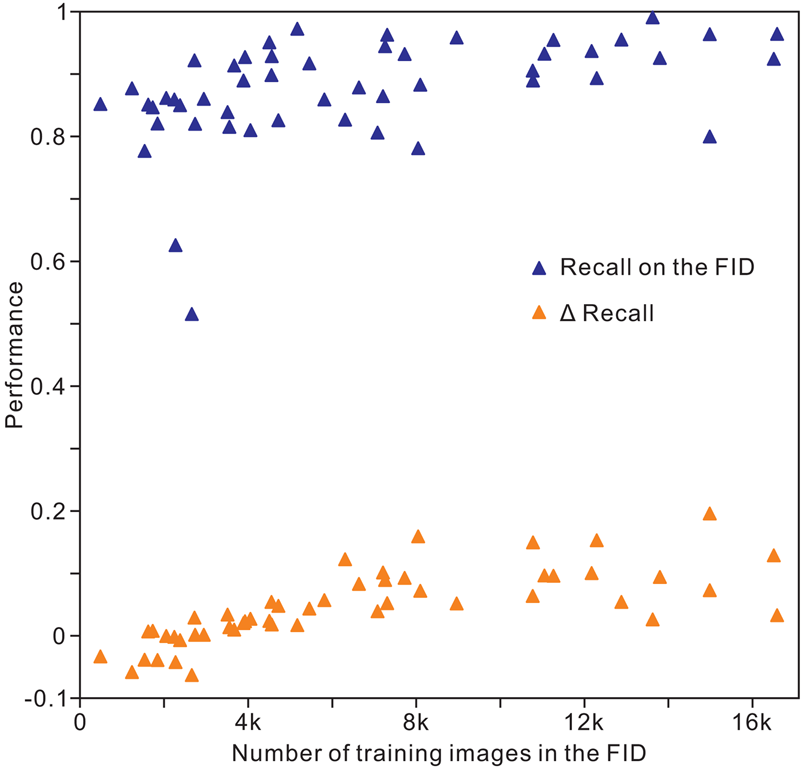
Figure 5. Distribution of individual clade recall with the volume of training images in the Fossil Image Dataset (FID). Δrecall equals accuracy on the FID minus accuracy on the reduced FID.
Table 3. Optimum performance from experiment 10 of Inception-ResNet-v2, which analyzed validation and test datasets to reduce occasional fluctuations in data.

Given the false positives in the main categories of microfossils, plants, invertebrates, and vertebrates, the DCNN tends to learn the main morphological features of fossils. Specifically, the misidentified images usually occurred in a class with a higher morphological disparity, or it was difficult to learn the unique characteristics of a class due to the image quality, data volume, and some other adverse aspects, especially for sponges, bryozoans, bone fragments, and trace fossils. Sponges were frequently misidentified as corals (rate of 0.14), bone fragments (0.06), and trace fossils (0.04). Bryozoans were mostly misidentified as corals (0.12), trace fossils (0.05), and sponges (0.05). Mammalian tooth specimens were misidentified as bone fragments (0.08), reptilian teeth (0.04), and mammals (0.02) (Table 3). The confusion matrix of 50 clades is provided in Supplementary Table S2. Several groups with low identification performance were often confused with one another, such as sponges, bryozoans, trace fossils, and corals. In addition, fossil fragments can undermine the identification of other clades, such as bone fragments, teeth, and petrified wood.
Figure 6 demonstrates the average values of 50 clades and the five highest- and lowest-performing clades based on the ROC curve from the validation and test sets. The AUC result shows that although some of the samples were predicted incorrectly, they have a much higher sensitivity than negative samples, such as samples from sponges and bryozoans. The positive rates rapidly increased when the false-positive rates were still lower. The micro average ROC and macro average ROC were similar considering the volume of the validation and test sets and the moderate data imbalance. The ROC curves of the 50 clades considered in this study are shown in Supplementary Figure S2.

Figure 6. Receiver operating characteristic (ROC) curves of an average of 50 clades (dashed curves), the five highest, and five lowest classes from the validation and test datasets. AUC describes the area under the ROC curve. Ideally, an area close to 1 is the best scenario. Black dashed line comprises 0.5 ROC space, indicating a random prediction.
Discussion
Performance Analysis
We used the models that were first trained on the ImageNet (Deng et al. Reference Deng, Dong, Socher, Li, Li and Li2009) for transfer learning on the FID, and they exhibited outstanding results, which indicates that pretraining has been effective for applications in different recognition tasks (Wang et al. Reference Wang, Ramanan and Hebert2017; Willi et al. Reference Willi, Pitman, Cardoso, Locke, Swanson, Boyer, Veldthuis and Fortson2019), despite the fossil images being considerably different from the ImageNet samples (Yosinski et al. Reference Yosinski, Clune, Bengio and Lipson2014). Hence, feature extraction using a CNN has a high generalization ability in different recognition tasks (Zeiler and Fergus Reference Zeiler and Fergus2014; Pires de Lima et al. Reference Pires de Lima, Welch, Barrick, Marfurt, Burkhalter, Cassel and Soreghan2020). Our approach, which froze half of the network layers as feature extractors and trained the remaining layers, provides the best performance. Transfer learning is also susceptible to overfitting, which may lead to experiments in which fine-tuning of all layers is inferior to fine-tuning of the deeper half-layers. We explored data augmentation, dropout, regularization, and early stopping methods to prevent such a situation. The first two methods are effective. We found that a frequent learning rate decay and large training batch contribute to faster convergence and high accuracy. The optimization of hyperparameters is usually empirical (Hinz et al. Reference Hinz, Navarro-Guerrero, Magg and Wermter2018) and becomes less effective as training proceeds. Compared with the model trained on reduced FID, most of the individual class accuracies linearly increased with the volume of training images, and the correlation coefficient was 0.73. Some of the clades with fewer than 3000 training images in the FID exhibited inferior performance on the reduced FID, but all classes with more than 3000 training images improved their accuracy on the complete FID. Imbalanced data caused the algorithm to pay more attention to categories with more training data. Sampling methods are typically used for imbalanced learning (He and Garcia Reference He and Garcia2009). In reduced FID, we used random undersampling to remove the majority clades and used random oversampling to expand the minority clades (oversampling method only used for snake fossils). The results show that removing images from the majority leads to missing important content from the majority of clades, whereas oversampling is effective to a certain extent. Moreover, the dataset quality is important for accurate identification. The microfossils performed with high identification accuracy, because most of the specimens were collected from publication plates that provide images with less background and noise. Some fossils with poor preservation and few samples available performed poorly, such as bryozoans and sponges. The large intraclass morphological diversity of a clade (e.g., trace fossils and bone fragments) also undermined the identification accuracy, because it is difficult for the DCNN architecture to extract discriminative characteristics. For instance, trace fossils comprise coprolites, marine trace fossils, terrestrial footprints, and reptilian egg fossils, thus involving fickle morphologies and characteristics. Considering the data imbalance between these classes and with other groups, we did not further subdivide trace fossils into the four abovementioned classes.
Visual Explanation of Fossil Clade Identification
Although irrelevant background noise may pollute test images, the DCNN architecture can extract representative areas. Nevertheless, the most discriminating areas are generally local features in fossil images, as shown in the Grad-CAM results in Figure 7. The red (blue) regions correspond to a high (low) score for predicting the label in Grad-CAM considering the average activation of the 1536 feature maps from Inception-ResNet-v2. Normally, the attention area of each feature map can be focused on the limited or unique characteristics (Selvaraju et al. Reference Selvaraju, Das, Vedantam, Cogswell, Parikh and Batra2016). A similar pattern is observed in the feature maps (Fig. 8), and some of the feature maps highlight the umbilicus, ribs, and inner whorl of the ammonoid. In particular, Inception-ResNet-v2 identifies different structures for each feature map in deep layers. (e.g., layers of mixed_7a and mixed _7b). Some feature maps are highly activated in a region limited to several pixels, indicating feature maps focus on specific spatial positions of the original image containing representative high-level structures. This phenomenon can be explained by the inherent characteristic of DCNNs, which compress the size (length and width) and increase the number (channels) of feature images through repeated convolutions. The feature maps from different convolutional layers demonstrate that shallow layers are sensitive to low-level features, such as brightness, edges, curves, and other conjunctions (layers conv2d_3 and conv2d_5 in Fig. 8) (Zeiler et al. Reference Zeiler, Taylor and Fergus2011; Zeiler and Fergus Reference Zeiler and Fergus2014). Conversely, deeper layers detect complex invariant characteristics within classes or capture similar textures by combining some low-level features. The activation of a single feature map focused on a small area that should be class discriminative (Zeiler and Fergus Reference Zeiler and Fergus2014; Selvaraju et al. Reference Selvaraju, Cogswell, Das, Vedantam, Parikh and Batra2017), such as figures H, I, and J from layer mixed_6a in Figure 8.

Figure 7. Visual explanation of samples from the test set, including the original image, gradient-weighted class activation mapping (Grad-CAM) fused with the original image, and guided Grad-CAM. The lower rectangle shows the predicted label and its probability. U–X were predicted incorrectly, and their true labels are crinoid, sponge, trace fossil, and bivalve, respectively. The red (blue) regions correspond to a high (low) score for predicting contribution in Grad-CAM. Specimens are not to scale. The image URLs are provided in Supplementary Table S1.

Figure 8. Visualization of the feature maps of different layers from Inception-ResNet-v2. From convd2_3 to mixed _7b (Supplementary Fig. S1), layers become deeper. First column of each layer is the averaged feature map (A), and the remaining column feature maps are nine examples of this layer (B–J). The dimensions of convd2_3, convd2_5, mixed_5b, mixed_6a, mixed_7a, and conv_7b are 147 × 147 × 64, 71 × 71 × 192, 35 × 35 × 320, 17 × 17 × 1088, 8 × 8 × 2080, and 8 × 8 × 1536, respectively. A schematic of the Inception-ResNet-v2 architecture is provided in Supplementary Fig. S1. Yellow (blue) pixels correspond to higher (lower) activations.
The activation patterns and feature maps show that the DCNN architecture can capture the fine-grained details of different fossils. For instance, the discriminative features extracted from ammonoids are mainly concentrated in the circular features merging from the umbilicus, especially for shells decorated with strong ribs (Fig. 7A). The spiral nautiloids highlight the area that contains similar characteristics. The feature maps demonstrate that the umbilical area is highlighted even in the middle layers (e.g., layers of mixed_5b and mixed_6a). Gastropod spires and apices are usually highlighted in Grad-CAM, considering that they contain curves and structures with large curvatures. For bivalves and brachiopods, the ornamented features of shells, such as growth lines and radial ribs, were extracted as representative features (Fig. 7B,E). Surprisingly, the DCNN seems to pay more attention to the dorsal or beak area of the shells, especially for brachiopods. These areas not only reflect significant differences between bivalves and brachiopods but also attract the attention of taxonomists. Therefore, DCNNs can capture the characteristics of fossils that are of interest to paleontologists. For arthropods, DCNN can highlight two pincers in crayfish, whereas it mainly concentrates on the body and tail of prawns and the head and wings of insects. The DCNN architecture provides outstanding performance in identifying vertebrate fossils. Grad-CAM emphasizes the skull and trunk of the vertebrate fossils, where distinguishing characteristics are located, especially for terrestrial vertebrates. This result may partially be attributed to some images in the FID showing only skulls. Class discrimination may result from a combination of several localized features. For instance, images of osteichthyes frequently show high activation on the skull, fins, and caudal fin areas (Fig. 7N). This phenomenon is also determined by Inception-v3 trained on ImageNet. Olah et al. (Reference Olah, Satyanarayan, Johnson, Carter, Schubert, Ye and Mordvintsev2018) built blocks of interpretability for an image that contains a Labrador retriever and tiger cat. The corresponding attribution maps reflected semantic features in deep layers, such as the dog's floppy ears, snout, and face and the cat's head. Similarly, the implemented DCNN can extract multiple targets from an image. Three areas are highlighted, corresponding to three blastoid specimens in Figure 7, despite some of the fossils being fragments. This result was confirmed in the images from bone fragments, ophiuroids, and pteridophytes. For the misrecognized images, we cannot fully interpret classification based on the visualization maps, but Grad-CAM and guided Grad-CAM provide activation areas with a higher morphological similarity in the identified error labels for images such as those of a crinoid stem and straight-shelled nautiloid. The clump structure of coprolite (trace fossil) is similar to that of modern globular stromatolites in Shark Bay. In summary, a DCNN can effectively extract features from images. Some complicated texture features (e.g., complex curves and boundaries) and clade-specific structures are paid more attention to and used for decision making. The class activation and feature maps can help humans partially understand how they work on fossil images.
Selvaraju et al. (Reference Selvaraju, Cogswell, Das, Vedantam, Parikh and Batra2017) demonstrated four visualization maps, including Grad-CAM, guided Grad-CAM, deconvolution visualization, and guided backpropagation, and interviewed mechanical workers on Amazon, demonstrating the superior performance of guided Grad-CAM, given its resemblance to human perception. However, this type of interpretability may be fragile. For example, we cropped or covered (with white polygons) the region with high activation in the original images. Nevertheless, the model still correctly recognizes most of the specimens, although with a low probability. By contrast, the activation patterns of Grad-CAM and guided Grad-CAM change and become difficult for humans to interpret. Regions with low activation in normal images were activated for accurate identification, indicating that class discrimination is not unique or immutable. In another study, neurons in CNNs have been confused by similar structures. In ImageNet, dog fur and wooden spoons, which have similar texture and color, have activated the same neurons (Olah et al. Reference Olah, Mordvintsev and Schubert2017). Similarly, the red stitches in baseballs have been confused with the white teeth and pink inner mouth of sharks (Carter et al. Reference Carter, Armstrong, Schubert, Johnson and Olah2019). We found similar situations in images from the collected FID, as discussed earlier.
The 50 clades of fossils or fragments were successfully clustered (Fig. 9) using t-SNE. A total of 2000 test images exhibited 0.88 accuracy. Among them, the cluster of fossils with more affinity (or morphological) relationships was closer. Several superclusters were obtained, such as plants (classes 3, 22, and 35), vertebrates (classes 2, 4, 16, 26, 24, 30, 36, 39, 46, and 49), arthropods (classes 11, 23, and 27), fishes (classes 0, 12, 31, and 34), microfossils (classes 13, 19, 32, 37, and 43), teeth and bone fragments (classes 8, 25, 38, and 40), bivalves and brachiopods (classes 6 and 9), and the Asterozoa of starfish and ophiuroids (classes 29 and 44). We found that even for samples that seem to be clustered incorrectly, the predictions are not completely wrong. This condition may be critical, because CNNs have been used to quantitatively visualize the morphological characteristics of fossils or organisms (Esteva et al. Reference Esteva, Kuprel, Novoa, Ko, Swetter, Blau and Thrun2017; Cuthill et al. Reference Cuthill, Guttenberg, Ledger, Crowther and Huertas2019; Esgario et al. Reference Esgario, Krohling and Ventura2020; Liu and Song Reference Liu and Song2020). This case is not valid for a few specimens, such as the Nautilus specimen (class of 28) shown in Figure 9. The conical or cylindrical shell is similar to belemnite, but it is recognized correctly. This result suggests that flattening 3D feature maps into a 1D vector leads to the loss of spatial information. Moreover, the fully connected layer at the end of the DCNN architecture is important for the final classification. We also applied UMAP (McInnes et al. Reference McInnes, Healy and Melville2018) for dimensionality reduction and obtained similar results (Supplementary Fig. S3).
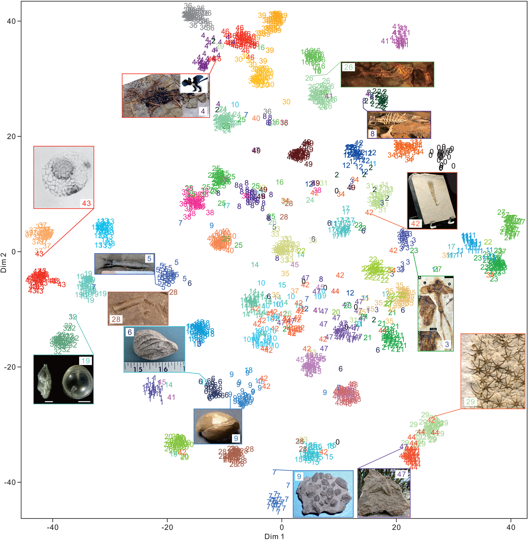
Figure 9. Feature visualization of the feature maps extracted from the final global average pooling layer of the Inception-ResNet-v2 architecture with 2000 random images (each class contains 40 images with 0.88 accuracy) in the test set using t-distributed stochastic neighbor embedding (t-SNE). The class order in alphabetical order is shown in Table 1. Some of the samples of clustering into other groups are shown in the rectangle with input images and their predicted labels. Specimens are not to scale. The image URLs are provided in Supplementary Table S1.
Considerable progress has been made in feature visualization over the past few years. The visual explanation provides a new perspective for understanding the workings of CNNs. However, the corresponding methods provide limited neuron interactions in CNNs (Olah et al. Reference Olah, Mordvintsev and Schubert2017), especially regarding quantitative visualization or morphological measurements.
Automatic Identification in Taxonomy
Recent studies on deep learning for genus- or species-level identification have mainly focused on modern organisms and a few microfossils, giving generally scarce data. Hence, existing studies have covered dozens of common species in a particular geological period (Keçeli et al. Reference Keçeli, Kaya and Keçeli2017; Pires de Lima et al. Reference Pires de Lima, Welch, Barrick, Marfurt, Burkhalter, Cassel and Soreghan2020). We expanded this type of research and identified 50 fossil (fragment) clades, rather than focusing on the identification of several species, and the identification performance seems comparable to that of human experts. We believe that under data scarcity, automatic taxonomic identification can be gradually enhanced from high-level identification toward genus-/species-level identification of specific groups. For example, if the FID is further labeled at the order, family, or genus level, then supervised taxonomic identification can be more detailed. However, image-based identification of fossil specimens has inherent limitations for some fossil groups. In fact, systematic taxonomists identify fossils not only by visual characteristics but also by considering additional structures, wall structures, and shell compositions of foraminifera, sutures in cephalopods, internal structures of brachiopods, and vein structures of leaves. Color images generally fail to reflect these features, making it difficult for DCNNs to detect them too. In our FID, images of sponges, bryozoans, trace fossils, and other clades showing various morphologies or with fewer training samples available led to inferior performance, indicating the difficulty of learning characteristics for these fossils compared with other clades. Pires de Lima et al. (Reference Pires de Lima, Welch, Barrick, Marfurt, Burkhalter, Cassel and Soreghan2020) also demonstrated that machine classifiers consistently misidentify some of the fusulinid specimens, because the wall structure is neglected. Piazza et al. (Reference Piazza, Valsecchi and Sottocornola2021) demonstrated a solution that used scanning electron microscopy images paired with a morphological matrix to recognize marine coralline algae. The matrix is connected with the flattened final feature maps and uses a fully connected layer for classification (Fig. 3). Thus, the chosen matrix is human intervention, which can add biotic or even abiotic information, but it loses the convenience of fully automatic implementation. In addition, to achieve species-level identification for certain fossil groups, other aspects should be considered, such as damaged specimens (Bourel et al. Reference Bourel, Marchant, de Garidel-Thoron, Tetard, Barboni, Gally and Beaufort2020) and the directions of thin-section specimens (Pires de Lima et al. Reference Pires de Lima, Welch, Barrick, Marfurt, Burkhalter, Cassel and Soreghan2020). Furthermore, secondary revision of the data collected from the literature is essential for the accurate supervision of deep learning (Hsiang et al. Reference Hsiang, Brombacher, Rillo, Mleneck-Vautravers, Conn, Lordsmith, Jentzen, Henehan, Metcalfe and Fenton2019). The taxonomic positions of some taxa may be modified in subsequent studies, it being necessary to coordinate classification criteria among scholars and research communities (Al-Sabouni et al. Reference Al-Sabouni, Fenton, Telford and Kucera2018; Fenton et al. Reference Fenton, Baranowski, Boscolo-Galazzo, Cheales, Fox, King, Larkin, Latas, Liebrand and Miller2018) for consistency. Even internal variations of taxa in different regions and periods should be considered, and DCNNs can also be used to verify these problems (Pires de Lima et al. Reference Pires de Lima, Welch, Barrick, Marfurt, Burkhalter, Cassel and Soreghan2020), given their highly accurate, reproducible, and unbiased classification (Renaudie et al. Reference Renaudie, Gray and Lazarus2018; Hsiang et al. Reference Hsiang, Brombacher, Rillo, Mleneck-Vautravers, Conn, Lordsmith, Jentzen, Henehan, Metcalfe and Fenton2019; Marchant et al. Reference Marchant, Tetard, Pratiwi, Adebayo and de Garidel-Thoron2020).
Deep learning may bring systematic paleontology to a new stage, and morphology-based manual taxonomic identification, including identification of microfossils and some invertebrate fossils, may soon be replaced by deep learning (Valan et al. Reference Valan, Makonyi, Maki, Vondráček and Ronquist2019). Experiments on invertebrate specimens demonstrate that the performance of deep learning is comparable to that of taxonomists (Hsiang et al. Reference Hsiang, Brombacher, Rillo, Mleneck-Vautravers, Conn, Lordsmith, Jentzen, Henehan, Metcalfe and Fenton2019; Mitra et al. Reference Mitra, Marchitto, Ge, Zhong, Kanakiya, Cook, Fehrenbacher, Ortiz, Tripati and Lobaton2019). With the continuous digitization of geological data, more fossil clades will be included and performance will improve. Although DCNNs cannot identify new species (supervised learning can only identify existing fossils, whereas unsupervised learning may detect anomalies or new species), they can accurately solve routine and labor-intensive tasks without the prior knowledge that taxonomists can only acquire after several years of training. Machine learning classifiers can help experts devote their time to the most challenging and ambiguous identification cases (Romero et al. Reference Romero, Kong, Fowlkes, Jaramillo, Urban, Oboh-Ikuenobe, D'Apolito and Punyasena2020). Recently, a single model was developed to identify thousands of common living plant species (Joly et al. Reference Joly, Bonnet, Goëau, Barbe, Selmi, Champ, Dufour-Kowalski, Affouard, Carré and Molino2016), which indicates that deep learning also has great potential in automatic taxonomy identifications. For our DCNN model to be publicly available, we deployed it on a web server, an uncommon practice in paleontology to date. Users can visit and use it at www.ai-fossil.com. The application of deep learning in paleontology benefits not only the academic community but also paleontological fieldwork, education, and museum collection management, spreading knowledge to the public. Furthermore, these applications can also provide more data for deep learning, and lead to more robust and accurate models.
Solutions to Data Scarcity
To our knowledge, this is the first time that web crawlers have been used or reported as being used in paleontology to collect image data for applications to automatic fossil identification based on DCNNs. This data-collection approach provides a new opportunity for disciplines in which massive training sets are difficult to obtain for developing deep learning. The hardware bottleneck of deep learning has mostly been overcome due to the dramatic increase in computing power of the graphics processor units, tensor processing units, and other artificial intelligence chips. However, the lack of large datasets poses a major obstacle for the application of deep learning in fields such as paleontology. We shared the FID, which can be reused in the future to train more powerful models and provide training data for genus/species identifications. Meanwhile, the trained model can be used for the rough identification of newly collected raw data, considering that data clearing/labeling is usually time-consuming.
With the increasing digitization and sharing of huge quantities of samples that have been housed in universities, research institutes, and museums and collected over the last three centuries, deep learning seems to be a promising research direction, and related efforts are underway, such as the Endless Forams (Hsiang et al. Reference Hsiang, Brombacher, Rillo, Mleneck-Vautravers, Conn, Lordsmith, Jentzen, Henehan, Metcalfe and Fenton2019) and GB3D Fossil Types Online Database (http://www.3d-fossils.ac.uk). Furthermore, the information age allows the use of diverse data sources through approaches such as citizen science data (Catlin-Groves Reference Catlin-Groves2012), which have been widely applied in biology through developments such as iNaturalist (Nugent Reference Nugent2018), e-Bird (Sullivan et al. Reference Sullivan, Wood, Iliff, Bonney, Fink and Kelling2009), eButterfly (Prudic et al. Reference Prudic, McFarland, Oliver, Hutchinson, Long, Kerr and Larrivée2017), and Zooniverse (Simpson et al. Reference Simpson, Page and De Roure2014). In addition, public data from the Internet could be considered. Alternatively, various algorithms reduce the need for massive sets of labeled data by adopting approaches such as unsupervised learning (Caron et al. Reference Caron, Bojanowski, Joulin and Douze2018), semi-supervised learning (Kipf and Welling Reference Kipf and Welling2017), and exploring deep learning on small datasets (Liu and Deng Reference Liu and Deng2015), likely accelerating the application of deep learning in paleontology.
Conclusions
In this study, we used web crawlers to collect the FID from the Internet to alleviate the data deficiency for fossil clade identification. The FID contains 415,339 images belonging to 50 fossil clades that can be used to train and evaluate three DCNN architectures. The Inception-ResNet-v2 architecture achieved 0.90 top-1 accuracy and 0.97 top-3 accuracy in the test set. We also demonstrated that transfer learning is not only applicable to small datasets but is also very powerful and efficient when applied to large data volumes (~106 samples). We conducted visual explanation methods to reveal discriminative features and regions for taxonomic identification using deep learning. The results revealed similarities between taxonomists and algorithms in learning and performing fossil image identification. Data scarcity has become a major obstacle to the application of deep learning in paleontology. With the digitization of dark data (i.e., unstructured data) and the collection of data from multiple sources, image-based systematic taxonomy may soon be replaced by deep learning solutions. Furthermore, we contributed a website for the entire community to access the models. We deployed the DCNN on a server for end-to-end fossil clade identification at www.ai-fossil.com.
Acknowledgments
We thank X. Dai for identifying cephalopods and for preparing the FID. We thank GitHub users for sharing the web crawler packages that we used to prepare the FID, including google-images-download (https://github.com/hardikvasa/google-images-download) from H. Vasa et al. and Bing image downloader (https://github.com/ostrolucky/Bulk-Bing-Image-downloader) from G. Ostrolucký et al. We thank all the web pages and sites that contribute to the FID. We declare that all the collected images are used for academic purposes only. We thank two anonymous reviewers for their insightful comments. This study is supported by the National Natural Science Foundation of China (41821001) and the Strategic Priority Research Program of the Chinese Academy of Sciences (XDB26000000). This is the Center for Computational & Modeling Geosciences Publication Number 5.
Data Availability Statement
Data available from the Dryad and Zenodo digital repositories: https://doi.org/10.5061/dryad.51c59zwb0, https://doi.org/10.5281/zenodo.6333970.


 Open access