


Introduction
Modern image acquisition in microscopy benefits greatly from the use of well-known focus stacking photomontage procedures. This often involves the taking of a set of images at successive focal distances, followed by mathematical processing and combining of the images to produce a resultant single image with an extended depth of field (DOF) [Reference Agarwala1]. This is useful when viewing subjects whose visible features lie at depths greater than the DOF of the objective lens in use or when objects are tilted or have irregular surfaces.
In the past, images to be included in a focus stack (stack) were taken one-at-a-time. A first image was taken, then the position of a subject relative to an objective lens was changed and a second image was taken, and so forth. This process has worked well, however it takes time.
This article describes an improved system for rapidly obtaining a set of images at video rates, that is, at tens of images per second and at different focal distances. The subject-to-objective focal distance remains constant so there is no movement of the microscope stage or objective. The new system greatly increases speed, convenience, and workflow in obtaining images with an extended DOF. The extended DOF brings life to moving and changing subjects and lets them be seen in the full context of their environment. The new system also applies to cameras, telescopes, binoculars, and monoculars [Reference Clark2, Reference Clark3].
Materials and Methods
Apparatus
Figures 1 and 2 show one arrangement of apparatus used for rapid acquisition of multiple images at different focal distances. In Figure 1, a lens with electrically variable focal length is secured to the trinocular port of a microscope, although it can just as easily be placed on an ocular port. A digital camera is secured to the variable focus lens (VFL) by an adapter such as a C- or F-mount. Electrical wires connect the camera and variable focus lens to control circuitry
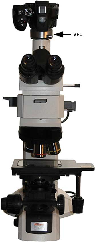
Figure 1 Components for rapid photomontage including the VLF lens.

Figure 2 A block diagram showing one arrangement of components required to produce a focus stack.
Figure 2 is a block diagram showing one arrangement of a control system for varying the focus of the VFL as a camera records images in preparation for focus stacking. The camera receives images from the microscope through the VFL, and the camera provides a synchronizing signal that causes the VFL to change focus for each image that is recorded. An high-definition multimedia interface (HDMI) cable connects the camera to a monitor that is used for setting variables such as the focus and VFL parameters. A vertical sync detector connected to the HDMI cable sends a signal to a microprocessor each time the camera sends an image to the monitor. The microprocessor is programmed to send signals to the VFL in order to vary its focal length in synchronism with the camera’s video rate. In the present case, the camera is free-running, recording and transmitting images at an internally selected rate. After acquisition, recorded images are delivered to a computer for processing.
Figure 3 is a photograph of the VFL that was used in this work [4,5]. The lens is plano-convex and has a focal tuning range of +45 to +125 mm. In the present work, we added a −100 mm offset lens to increase this range to −500 to +82 mm in order to enlarge the image on the camera’s sensor and reduce the deviation from the microscope optical design parameters. The VFL is driven by a current source, and its focal power in diopters (dpt) is linear with applied current. From zero to maximum current, the focal power of the combined lenses ranges from −2 to +13 dpt. The transient response of the lens is sufficiently fast to permit operation at 60 Hz, the progressive video refresh rate of the camera used in this work.

Figure 3 The VFL and lens mount adapter used in this work.
Method
Figure 4 shows the focal power of the combined VFL and offset lens as a function of current. The focal power increases linearly with increasing current. In the apparatus described here, the VFL is located at the exit of the microscope’s trinocular port. Placing the VFL here causes changes in magnification and field of view (FOV) as the focal length of the VFL is varied [5]. In focus stacking, magnification changes that occur with changing focal length of the VFL are generally removed during processing by the focus stacking software.

Figure 4 The VFL focal power as a function of current.
Figure 5 is a plot of VFL current versus time during capture of a stack that will form a single image. In the present work, the timing is supplied by a digital single-lens reflex (DSLR) camera operating in video mode. The VFL current is set to a different value for each time slot, that is, t0 to t1, t1 to t2, and so forth. The timing of image capture is marked by asterisks. Capture occurs near the end of each current step to allow settling of the lens at one end and time for image transfer from the camera’s sensor to memory at the other. The values of current are selected so that the DOF at each current overlaps the DOF at the next current. Minimizing the overlap from one current value to the next hastens image capture and reduces the number of images acquired in a stack, which in turn minimizes the amount of image processing required to form a final image.
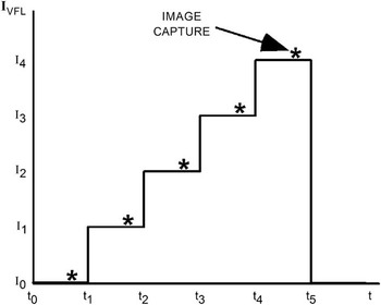
Figure 5 A plot of VFL current vs. time.
Setup
Prior to recording a series of images, values for I0, I4, and the number of steps, N, between I0 and I4 are determined. The height of the specimen to be examined is determined manually using the microscope’s calibrated focusing knob or other means.
1. With the lens current at I0 (I0=0 in most cases), the camera’s “live view” mode is used to manually focus the microscope on the lowest point in the specimen.
2. Next, the lens current is manually increased until the highest point in the specimen is in focus. This current is I4.
3. The height of the specimen is divided by the DOF of the objective lens being used. The quotient is N, the minimum number of images to be included in the focus stack.
4. The values for I0, I4, and N are entered into the microprocessor’s program.
5. The camera’s video recording function is started and runs until images for all N steps are recorded. In the present example, 5 images are recorded, each at a different focal depth. The camera used in this work records 60 images per second, so all 5 images for a stack are recorded in 5/60=83 ms.
For routine work I0, I4, and N are pre-assigned values and are held in the microprocessor’s memory as constants. When an objective is changed, only N is updated so that setup time is minimized. The above setup steps can easily be automated. In the present apparatus, I4 and N can be conveniently changed on the fly.
Figure 6 shows the steps in processing of a stack of images. A stack of images is saved either in the camera’s memory or in the computer. A focus stacking program [6, 7] extracts the in-focus parts of each image in the stack and combines them into a final, all-in-focus image.

Figure 6 A flow diagram showing the steps in processing a stack of images.
Video image capture
The above techniques are easily applied to video image capture. Figure 7 is a plot of VFL current versus time during capture of a multi-frame video stream. The VFL current IVFL cycles through all values once per frame. In this case, instead of returning to zero at the end of a frame as shown in Figure 5, IVFL reverses direction with each frame. This is because smaller current steps have a shorter transient response from one value to the next, thus enabling a higher video rate. The stack of images captured in each frame is processed into a single resultant image per frame. The processed images are displayed one at a time on a monitor, or they can be combined to form a movie. The speed of image capture is limited only by image acquisition time and refocus time.
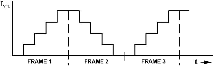
Figure 7 A plot of VFL current vs. time in video mode.
Regions of interest
In some applications only a limited number of regions of interest (ROI) are required. Individual images in each ROI can be selected from a larger stack, such as would be obtained using the timing in Figure 5, while images that are not selected are ignored. However, images that are ignored represent time wasted in the gathering of image data. Instead, image acquisition time is shortened by acquiring only images of interest. Figure 8 shows the timing of lens focusing currents for 2 ROIs. Images in ROI #1 are captured at times between t0 and t2, while images in ROI #2 are captured at times between t2 and t4. No image is acquired at currents between I1 and I2, thus no time is wasted by gathering an image that will be ignored. Individual ROIs are processed separately in focus stacking software, as discussed below.

Figure 8 A plot of VFL current vs. time. Regions of interest are selected.
Results
Circuit board
Figure 9 shows images of a component on a printed circuit board. The height of the component is 1,118 microns, and the DOF of the 5× objective used here is 44 microns. The FOV is 3.0 mm. The calculated number of images required for focus stacking, N, is 25. A total of 27 images were acquired to allow some DOF overlap. Left to right: in the first image, the printed circuit board and solder connections are in focus. The next image is number 14 in the stack, and the focus is halfway to the top of the component. The third image is number 27, and the focus is at the top of the component. The fourth image is the resultant processed, all-in-focus image. All images were captured in 0.45 sec.

Figure 9 The circuit board. Left to right: the circuit board in focus, halfway between the circuit board and the top of the component, the top of the component, and the processed image completely in focus. 5× objective, stack of 27 images, final image diameter ≅3.0 mm, acquisition time=0.45 sec.
Ronchi ruling
Figure 10 shows the setup used in photographing a tilted subject. A 250 lp/in, chrome-on-glass Ronchi ruling, a lined resolution test target [8], was tilted at about 10 degrees with respect to the microscope stage and illuminated diascopically. A10× objective lens with a DOF of 8 microns was used, and its FOV was 1.5 mm. The height difference across the FOV was 300 microns, thus a minimum of 37 images were required for a stack. A total of 38 were used. All images were captured in 0.63 sec. Figure 11 shows successive images of the Ronchi ruling. Left to right: the first image shows image number 1 taken with focus at the left-hand end of the FOV. The next image is number 19, and the focus is at the center of the FOV. The third image is number 38, with focus at the right-hand end of the FOV. The fourth image is the resultant processed, all-in-focus image.

Figure 10 Ronchi ruling setup. The ruling is tilted 10 degrees.

Figure 11 Ronchi ruling. Left to right: image focused at the left, image focused at the center, image focused at the right, processed image completely in focus. 10× objective, stack of 38 images, final image diameter ≅1.5 mm, acquisition time = 0.63 sec.
Mammalian tissue
Figure 12 shows successive images of a diascopically illuminated stained mammalian tissue specimen. The FOV is 0.3 mm, the thickness of the specimen is 15 microns, and the DOF of the 50× objective used here is 1.18 microns. A total of 15 images were acquired at 60 Hz for a total acquisition time of 0.25 sec. Two features, A and B, are noted in the images. In image 1, focused on the lowest part of the specimen, feature A is visible, and feature B is barely discernible. In image 7, focused halfway between the lowest and highest parts of the specimen, feature A is less visible, and feature B is partially visible. In image 15, focused at the highest part of the specimen, feature A is nearly invisible, and feature B is clearly visible. Both features are easily seen in the final stacked image. With a fixed focus, a viewer or an automated image analyzer could easily miss one or the other of these features, but with focus stacking, both are easily seen.

Figure 12 Mammalian tissue specimen. Image 1 is focused at the lowest level where feature A is in focus. Image 7 is focused near the center of the specimen. Image 15 is focused at the top where feature B is in focus. Image All is a processed image showing all features in focus. 50× objective, stack of 15 images, final image diameter ≅0.3 mm, acquisition time = 0.25 sec.
Discussion
Note that the focus stacking software was able to properly scale the individual images in spite of the apparent change in scale and FOV as the VFL current was varied. Thus, despite the large height of the circuit board and ruling specimens, it was not necessary to scale the images before processing the stack. In our experience, feature tracking and scaling within the stacking software works very well except when there are discontinuities in specimen height across the FOV.
When separate ROIs are imaged as described in connection with Figure 8, a discontinuity in specimen height occurs. The magnifications in the two ROIs are different, and the focus stacking software has no image features to follow from one image to the next in order to provide proper scaling of the images with respect to one another. The resultant image shows the two ROIs at two different magnifications. This discrepancy is easily removed by doing a one-time calibration of the magnification versus lens current. If ROI #1 is used as a standard, images acquired in ROI #2 are simply scaled by the new magnification factor prior to focus stacking.
Focusing without changing magnification and FOV can be done, however this is generally not possible with most commercial microscopes. It requires placing the VFL in a part of the optical path that is not usually reachable [5].
We have demonstrated a system for rapid acquisition of images for focus stacking. The DOF of a lens system and the height of a specimen determine the minimum number of images required to obtain an all-in-focus image. Synchronizing lens focus with image capture and selecting only the minimum required number of overlapping DOF images minimizes the time required to acquire images for processing by focus stacking. The speed of image capture is limited only by the camera and the VFL. Instead of synchronizing focusing with the camera, a controller can trigger the camera in sync with changing focal lengths of the VFL. A number of VFL technologies are available, and some may be suited to particular applications [9-11].
Other methods for changing focal distance are used in microscopy. In one, a microscope objective lens is moved up and down. In another, a focusing stage moves the specimen up and down [12]. These mechanical methods offer tradeoffs to the VFL approach: the magnification at the focus remains constant with changing distances between an objective lens and a specimen. But this is not a problem with focus stacking because stacking software identifies and aligns features in each image of a stack by digitally scaling the images. An advantage of a VFL over a moving objective lens is that the VFL is easily inserted between a microscope’s trinocular port and a camera. This allows use of a microscope’s lens turret to quickly select among different objectives. Another advantage of a VFL over mechanical systems is speed. The step response settling time of a VFL is generally shorter than found in a mechanical system. This means that multiple image acquisition can be faster with a VFL than with a mechanical system.
Acquiring images at the maximum possible speed improves work throughput and permits the all-in-focus imaging of moving or changing specimens. Microscopic species can be viewed in a three-dimensional environment, instead of being squeezed between a microscope slide and a cover slip to keep them in focus. Time-lapse imaging of crystal growth or other morphological changes of substances can be done. Inspection of tilted objects is easily done. Machine vision and inspection can benefit both in speed and image quality from the technology described here. Limited 3D capability is also available in focus stacking software [6, 7]. Additional images are available for viewing on our website [13].
Although we have improved the rate of image capture, the speed of image processing by focus stacking has room for improvement. The stack of 15 images in Figure 12 was acquired in 0.25 seconds but required about 6 seconds to process in a reasonably fast desktop personal computer. For this reason, ongoing work includes assembling a fast video processor for image capture, focus control, and focus stacking [Reference Clark2, Reference Clark3].
Conclusion
This article describes a new method that can rapidly acquire focus stacks in less than a second. Processing the focus stack on a personal computer, to produce an image with apparent large DOF, currently takes about 20 times longer than the acquisition time.


