


1. Introduction
Free shear flows can be considered as one of the driving research topics in fluid mechanics. Their vast application ranges from the understanding of fundamental mechanisms such as turbulence production and decay (Dairay, Obligado & Vassilicos Reference Dairay, Obligado and Vassilicos2015; Zhou et al. Reference Zhou, Nagata, Sakai, Ito, Terashima and Hayase2018, Reference Zhou, Nagata, Sakai and Watanabe2019; Cafiero & Vassilicos Reference Cafiero and Vassilicos2019), modelling of mixing in rivers and estuaries (Stansby Reference Stansby2003; Cafiero & Woods Reference Cafiero and Woods2016), application for flow control and drag reduction (Dghim, Ferchichi & Fellouah Reference Dghim, Ferchichi and Fellouah2018; Cannata, Cafiero & Iuso Reference Cannata, Cafiero and Iuso2019) and heat transfer enhancement (Carlomagno & Ianiro Reference Carlomagno and Ianiro2014; Cafiero et al. Reference Cafiero, Castrillo, Greco and Astarita2017), to cite some.
Regarding the last topic mentioned above, significant effort has been spent to determine effective ways to improve the convective heat transfer capabilities of jets in the impinging configuration. This is often quantified in terms of the Nusselt number  $Nu=hD/k$, where
  $h$ indicates the convective heat transfer coefficient,
  $D$ is a reference length scale such as the nozzle exit diameter and
  $k$ is the fluid thermal conductivity. The main fluid dynamics parameters on which
  $Nu$ depends are the Reynolds number and the turbulence intensity level of the flow (Hoogendoorn Reference Hoogendoorn1977; Carlomagno & Ianiro Reference Carlomagno and Ianiro2014). The key is then to modify these parameters to cater for higher convective heat transfer rates.
Some of the most significant solutions aimed at achieving this goal are acoustic excitation (Tianshu & Sullivan Reference Tianshu and Sullivan1996), application of a swirl component to the mean flow (Huang & El-Genk Reference Huang and El-Genk1998; Ianiro & Cardone Reference Ianiro and Cardone2012), introduction of streamwise vortex generators (Violato et al. Reference Violato, Ianiro, Cardone and Scarano2012), introduction of perforated plates between nozzle and target plate (Hee Lee et al. Reference Hee Lee, Min Lee, Taek Kim, Youl Won and Suk Chung2001) or installing mesh screens within the nozzle (Zhou & Lee Reference Zhou and Lee2004). A common feature amongst all the proposed solutions is that the heat transfer enhancement is obtained by either exciting or altering the structure and organization of the turbulence produced in the near field. Modifying the large coherent turbulent structures can provide significant benefits in terms of heat transfer enhancement.
In a recent experimental investigation of free and impinging jets (Cafiero, Discetti & Astarita Reference Cafiero, Discetti and Astarita2015; Cafiero et al. Reference Cafiero, Greco, Discetti and Astarita2016) it has been shown that the introduction of square fractal grids (i.e. grids obtained by repeating the same initial pattern at increasingly smaller scales) leads to a significantly higher entrainment rate compared to jets without turbulators. This is achieved by a significant alteration of the near field of the flow. Consistent with the higher entrainment rate, Cafiero, Discetti & Astarita (Reference Cafiero, Discetti and Astarita2014) and Cafiero et al. (Reference Cafiero, Castrillo, Greco and Astarita2017) showed that the use of fractal grids has a significant effect on the convective heat transfer rate, especially at short nozzle-to-plate distances.
Square fractal grids have been widely investigated in the past decade for their peculiarity in terms of turbulence production and decay (Hurst & Vassilicos Reference Hurst and Vassilicos2007; Mazellier & Vassilicos Reference Mazellier and Vassilicos2010; Gomes-Fernandes, Ganapathisubramani & Vassilicos Reference Gomes-Fernandes, Ganapathisubramani and Vassilicos2012; Nagata et al. Reference Nagata, Saiki, Sakai, Ito and Iwano2017). Given the multiscale structure of the grid, the underlying mechanism leading to turbulence production is quite different from that typical of regular grids. In particular, the turbulence is produced by the interaction of the wakes shed by the single grid elements, which will meet at different downstream distances. This results in an elongated turbulence production region (Mazellier & Vassilicos Reference Mazellier and Vassilicos2010). More importantly, the turbulence production region extent depends on the grid geometry, through the wake interaction length scale defined as  $x^*=L_0^2/t_0$, where
  $L_0$ is the side of the largest grid element and
  $t_0$ is its thickness. Such scaling parameter is defined by scaling the half-width of the wake
  $y_{1/2} \sim \sqrt {t_0x}$ following Townsend (Reference Townsend1976). Considering the wake of the largest bars only, the wake-interaction length scale
  $x^*$ is defined as
  $L_0 =y_{1/2} \sim \sqrt {t_0 x^*}$ (Mazellier & Vassilicos Reference Mazellier and Vassilicos2010).
Despite the large body of research carried out on the topic, there is still a lack of a thorough analysis of the flow-field structure and properties in the near field of a jet with fractal turbulators. The previous experimental efforts were carried out at resolutions that hindered the sampling of the underlying phenomenon occurring in the lee of the grid. Hence, the points that we want to address in this paper are the following: Is there any dependency of the grid thickness ratio on how the turbulence is produced, transported and dissipated? Is it possible to design bespoke fractal grids optimizing the value of the thickness ratio? What is the effect of adding secondary grid iterations on turbulence production, transport and dissipation? In their work, Cafiero et al. (Reference Cafiero, Discetti and Astarita2014) and Cafiero et al. (Reference Cafiero, Castrillo, Greco and Astarita2017) showed that fractal grids can achieve significantly higher values of the convective heat transfer rate compared with regular and single square grids. What is the underlying mechanism leading to such enhancement? The outcomes of these questions would provide significant insights into the mechanism connected to multiscale grids, providing fundamental grounds to the findings of Cafiero et al. (Reference Cafiero, Castrillo, Greco and Astarita2017) and benefiting the community interested in grid-generated turbulence in jets.
The paper is organized as follows. We start by describing the experimental apparatus and the particle image velocimetry (PIV) process in § 2. The mean flow properties are then discussed in § 3.1, with a particular focus on the main terms of the one-point turbulent kinetic energy equation in § 3.2. The flow-field structure is then analysed using a low-order approach in § 3.3. The main conclusions are drawn in § 4.
2. Experimental set-up
Air is collected from the environment with a centrifugal blower. An inverter is used to regulate the input shaft angular velocity. The fluid is seeded with olive oil particles (used as tracers) generated by means of a Laskin nozzle (Raffel et al. Reference Raffel, Willert, Wereley, Kompenhans, Willert, Wereley and Kompenhans2007). The flow rate is measured through a rotameter while a heat exchanger is used to reduce to a minimum the fluid temperature variations with respect to the surrounding environment. The fluid is conveyed through a plenum chamber (whose internal diameter and length are, respectively, equal to 3 $D$ and 20
 $D$,
$D$,  $D=20$ mm being the nozzle diameter) located upstream of a short pipe nozzle which is 6.2
 $D$ long. Inside the chamber two honeycombs reduce the large flow structures that may be generated within the feeding circuit. A contoured entrance is used to carry the air through the short pipe nozzle and a terminating cap is eventually used to locate the grid at the nozzle exit section. The experiments are carried out in a room where the temperature is regulated and kept constant, to ensure minimum variation of the air properties. The Reynolds number is kept constant and equal to
  $Re=U_bD/\nu =16\ 000$, where
  $U_b$ is the bulk velocity.
A family of fractal grids (FGs) and two single square grids (SGs) are employed for this set of experiments and are compared with both the jet without turbulator (JWT) and the regular grid (RG). The FG geometries are characterized by the largest grid item length  $L_0$ and thickness
  $t_0$, along with the thickness and length ratios
  $t_r=t_0/t_{N-1}$ and
  $L_r=L_0/L_{N-1}$, with
  $N$ the number of iterations. Length and thickness at the
  $j$th iteration can be obtained as
  $L_j=L_0 R_L^j$ and
  $t_j=t_0 R_t^j$, where
  $R_L$ (
 $R_t$) indicates the ratio between the length (thickness) of two consecutive iterations. In the present case, all the FGs have a number of iterations
  $N=3$. The grid blockage ratio
  $\sigma$ is defined as the ratio between the obstructed area over the overall nozzle exit section area. The single square grids SG1 and SG2 are directly derived by FG2 by removing the second and third iterations and, therefore, have a blockage ratio which is one-third of that of the FGs. They differ by the orientation of the holding bars: in the former case, the holding bars are directed along the diagonal of the central grid item; in the latter, the holding bars are orthogonal to the central grid item. All the relevant geometric parameters are summarized in table 1. A schematic representation of a three-iteration FG is reported in figure 1(a).

Figure 1. (a) Fractal grid geometric parameters. (b) Schematic representation of the experimental set-up.
Table 1. Geometric details of the grids. Grids SG1 and SG2 differ by the orientation of the holding bars: in the former case, the holding bars are directed along the diagonal of the central grid item; in the latter, the holding bars are orthogonal to the central grid item.

A sketch of the experimental set-up is shown in figure 1(b). A Quantel Evergreen laser for PIV applications (532 nm wavelength, 200 mJ pulse $^{-1}$,
  $<$10 ns pulse duration), with an exit beam diameter of about 5 mm, is used to illuminate the measurement domain. The laser beam is initially enlarged by means of a bi-convex spherical lens (with
  $-$25 mm focal length) and then adjusted by a bi-concave spherical lens (with 75 mm focal length). A
  $90^{\circ }$ rotation directs the laser beam towards the measurement region. Finally, a second bi-convex spherical lens (with 300 mm focal length) and a cylindrical lens (with
  $-$50 mm focal length) are used to obtain the laser sheet. The laser is operated in double-pulse mode, with a time delay between the two pulses of 16
  $\mathrm {\mu }$s and acquisition frequency set to 15 Hz.
The origin of the reference frame corresponds to the centre of the round nozzle exit section. The  $x$ axis is aligned with the jet centreline while
  $y$ is perpendicular to
  $x$, in the vertical direction. Concerning the FGs and the SGs, all the grids are analysed along both the
  $xy$ plane (whose results will be denoted by
  $-$0) and the plane rotated by 45
 $^{\circ }$ with respect to it (whose results will be denoted by
  $-$45).
Four Andor Zyla sCMOS 5.5 Mpixels cameras are used to image an area extending for  $8D$ in the streamwise direction starting from the nozzle exit section and
  $1.5D$ in the cross-stream direction symmetrically located with respect to the nozzle axis, thus effectively covering
  $\pm 0.75D$. Each camera is equipped with a 100 mm Tokina macro-objective operated with an aperture set to
  $f_\#= 16$. A spatial resolution of 60 pixels mm
 $^{-1}$ is obtained locating the four cameras alternately on either side of the laser sheet. A sufficient number of overlapping pixels are considered to perform a reliable stitching of the images captured by consecutive cameras. In order to reduce to a minimum any spurious noise, this operation is carried out at raw image level, correlating the velocity fields from consecutive cameras.
For each grid as well as for the JWT, 6000 instantaneous PIV realizations are acquired, along both the  $0^{\circ }$ and the 45
 $^{\circ }$ directions, in order to assess the streamwise evolution of the flow field. The number of snapshots is chosen in a way such that the margin of error is 0.2 % and 3 % on the mean flow and standard deviation, respectively, with a 99 % confidence interval.
A spline interpolation of the preprocessed images as well as of the velocity field is operated as recommended by Astarita (Reference Astarita2006, Reference Astarita2008). A Blackmann weighting window is applied to the final window to tune the spatial resolution of the resulting velocity field (Astarita Reference Astarita2007). The final interrogation window size is set to  $24 \times 24$ pixels, with 75 % overlap, resulting in a vector pitch of 0.1 mm. In terms of relevant flow scales, the pixel pitch corresponds to
  $\approx 7\eta$ in the worst-case scenario, where
  $\eta =(\nu ^3/\varepsilon )^{1/4}$ is the Kolmogorov length scale,
  $\varepsilon$ the turbulence dissipation and
  $\nu$ the air kinematic viscosity. As worst-case scenario we consider the region of the flow where the dissipation is the highest, i.e. immediately past the central grid item. In the case of the JWT, near the nozzle exit section the flow is mostly laminar, so the relevant length scale is the shear layer thickness. We estimated the shear layer thickness at
  $x/D=0.05$, from the time-averaged vorticity profile. We measured the distance between two consecutive zero crossings of the vorticity profile, respectively occurring in the irrotational flow region (outside the jet core) and in the potential core of the jet. This scale was significantly larger than
  $\eta$, being of the order of 0.15
 $D$.
$D$.
We performed an estimate of the error associated with the PIV process measuring the displacement field in pixels obtained in regions where the flow is quiescent. This resulted in a value of about 0.15 pix, which in turn corresponds to a 1.5 % error in the estimate of the mean flow.
2.1. Comparison with previous literature
We performed a validation of the experiment by comparing the results obtained in the JWT case with literature data. Figure 2 shows the mean and root mean square (r.m.s.) of the streamwise velocity component measured at  $x/D=0.05$ in the JWT case. Data are normalized with respect to the centreline velocity
  $U_c$. We compared our results with those obtained by Mi, Nobes & Nathan (Reference Mi, Nobes and Nathan2001), which are taken at the same Reynolds number (16 000) and at the same location, but with different inlet conditions, namely a pipe nozzle and a contraction, as opposed to the short pipe nozzle employed in the present experiments. As expected, the inlet profiles obtained with a short pipe nozzle sit between the two reference cases. In particular, the mean velocity
  $\bar {U}/U_c$ resembles quite closely the top hat profile obtained with the contraction inlet. Conversely, the inlet profile obtained in the pipe case approximates a fully developed parabolic profile.

Figure 2. (a) Mean streamwise velocity and (b) r.m.s. of the streamwise velocity profiles measured at  $x/D=0.05$ and normalized with respect to the centreline velocity value
  $U_c$. Data are compared with the measurements of Mi et al. (Reference Mi, Nobes and Nathan2001) taken at the same Reynolds number (16 000) for different inlet conditions, namely a contraction and a pipe nozzle.
The r.m.s. of the streamwise velocity component features values close to zero within the potential core, as in the contraction case. However, a broader shear layer can be clearly detected following the partial flow development occurring within the short pipe nozzle. This is also confirmed by the even wider shear layer that is obtained in the pipe case.
3. Results and discussion
3.1. Mean flow spatial organization
We start by showing the mean flow spatial organization for all the investigated cases, with the aim of giving a direct grasp of the effect of the thickness ratio and of the secondary iterations on the flow field.
Figures 3–5 report the time-averaged axial velocity contour maps relative to the SGs, the FGs and the RG, respectively. It is worth noticing that, in order to reduce the measurement noise, their values are averaged with respect to the symmetry plane  $x$–
$x$– $z$.
$z$.

Figure 3. Time-averaged axial velocity component contour maps relative to the SGs.

Figure 4. Time-averaged axial velocity component contour maps relative to the FGs.

Figure 5. Time-averaged axial velocity component contour map relative to the RG.
Figure 3 shows that the effects associated with the different holding bars can only be appreciated close to the nozzle exit section, as they affect the recirculation region evolution, while no significant differences can be observed in the axial velocity values, consistent with their equal blockage ratio. On the other hand, according to the higher value of the blockage ratio  $\sigma$ (which is almost three times the blockage ratio of the SGs), all the maps relative to the FGs (see figure 4) are characterized by higher velocity values with respect to those of the SGs.
As expected, the different thickness of the grid items influences the jet evolution close to the nozzle exit section, so that, in the 0 $^{\circ }$ maps, a higher value of
  $t_0$ corresponds to a more extended recirculation region past the first iteration grid item. On the other hand, less fluid moves through the secondary iteration squares. Therefore, the axial velocity distribution shows higher uniformity for decreasing
  $t_r$ values as the blockage imposes on the flow a more even distribution.
As observed in Cafiero et al. (Reference Cafiero, Castrillo, Greco and Astarita2017) in the case of impinging circular jets equipped with fractal turbulators, this affects the convective heat transfer rate and, more importantly, its spatial uniformity. The authors showed that FG inserts are indeed extremely effective in getting localized high convective heat transfer rate at short nozzle-to-plate distances. Conversely, the use of a single SG, or the choice of a different initial pattern, is advised when it is desirable to obtain a uniform distribution of the convective heat transfer rate.
Moving downstream, the jet loses memory of the grid geometry and no significant difference between the investigated cases can be perceived for  $x/D>7$.
Figure 5 reports the time-averaged axial velocity contour maps past the RG. Since the laser sheet is directed along one of the grid's bars, an initial velocity defect can be detected. As  $x/D$ increases, the axial velocity is recovered. For
  $x/D<2.5$, the highest axial velocity values are located at the interface between the core of the jet and the growing shear layer.
The time-averaged axial velocity profiles evaluated along the centreline for all the analysed grids are shown in figure 6. The data for the JWT case are also plotted as reference. Both single and fractal square grids cause a significant increase of the mean axial velocity immediately past the grid, as a consequence of the local blockage imposed by the grid iterations. Both the  $\bar {U}/U_b$ profiles for the SGs attain values of about 1.5 at
  $x/D=0.05$ with a rapid decrease that leads to values smaller than the JWT cases from 4
 $D$ and 4.65
 $D$ from the nozzle exit section, respectively, for SG1 and SG2.

Figure 6. Time-averaged axial velocity profile  $\bar {U}/U_b$ evaluated along the jet centreline (
 $y/D=0$).
The length of the measurement domain is not large enough for complete jet development past both SG1 and SG2. Therefore, the velocity profiles do not recover the behaviour of the JWT flow field.
An increase of  $t_r$ from 2.04 to 6.25 in the FGs causes an increase of the mean axial velocity at short distances from the nozzle, because of the progressively smaller area through the central grid item. Nevertheless, this mechanism is not monotonic, as the largest value is attained for the FG2 case. A similar behaviour was observed for the convective heat transfer rate (Cafiero et al. Reference Cafiero, Castrillo, Greco and Astarita2017).
Finally, independent of the inlet conditions, all the curves practically collapse to that of the JWT for  $x/D>7$.
Figure 6 also shows that the streamwise velocity measured in the lee of both the SGs and FGs reaches a local minimum between  $0.4<x/D<0.5$. This initial reduction of the mean streamwise velocity could be associated with a vena contracta effect, according to results reported by Quinn & Azad (Reference Quinn and Azad2013) for sharp-edged-orifice round and cruciform jets.
The RG mean axial profile strongly differs from those described above. As already suggested by the contour map (see figure 5), after an initial recovery,  $\bar {U}/U_b$ attains a constant value of about 1.4 for
  $1<x/D<5.5$ and it then decreases. Different from the SG profiles, apart from the initial stage,
  $\bar {U}/U_b$ always shows higher values than the JWT. This difference is expected to decrease at larger distances, where the effect of the grid fades out.
The r.m.s. axial ( $u^{\prime }/U_b$) and the radial (
 $v^{\prime }/U_b$) velocity fluctuations evaluated along the jet centreline are reported in figures 7(a) and 7(b). The profiles show two peaks: a first one at smaller values of
  $x/D$, which we attribute to the grid-generated turbulence, and a second one at larger streamwise distances, which is related to the effect of the growing jet shear layer merging at the centreline. According to Seoud & Vassilicos (Reference Seoud and Vassilicos2007), Mazellier & Vassilicos (Reference Mazellier and Vassilicos2010) and Nagata et al. (Reference Nagata, Saiki, Sakai, Ito and Iwano2017), both the number of fractal iterations and the bar thickness affect the turbulence intensity peak, in the case of grid-generated turbulence. Starting from the momentum equation of a wake in the far field, Gomes-Fernandes et al. (Reference Gomes-Fernandes, Ganapathisubramani and Vassilicos2012) obtained a scaling of the turbulence intensity peak based on the drag coefficient of the grid and the thickness of the central grid item. A comparison between SGs and FG2 (i.e. the square FG having the same
  $L_0$ and
  $t_0$ values) shows that the increase in
  $N$ causes an upstream shift of the location of the peak (
 $x_{peak}$), in good agreement with the decaying grid turbulence measurements reported by Mazellier & Vassilicos (Reference Mazellier and Vassilicos2010) and Nagata et al. (Reference Nagata, Saiki, Sakai, Ito and Iwano2017), for
  $1\leq N\leq 3$. This suggests an effect of the secondary grid iteration on the location of the maximum value of the turbulence intensity. Nevertheless, it is worth explicitly pointing out that the comparison in terms of maximum turbulence intensity between the FGs and the SGs is not meaningful given the significantly different value of the blockage ratio. Similarly to the convective heat transfer results reported by Cafiero et al. (Reference Cafiero, Castrillo, Greco and Astarita2017), only small differences can be detected between FG1 (
 $t_r=6.25$) and FG2 (
 $t_r=4.05$). To investigate this aspect further, in figure 8 we plot the value of the turbulence intensity peak, defined as the maximum value of
  $tke=\frac {1}{2}({u^{\prime }}^2+2{v^{\prime }}^2)$ (with
  $v^{\prime }=w^{\prime }$ at the centreline) in the range of streamwise distances
 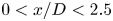 $0<x/D<2.5$ as a function of
  $t_r$. The peak in the turbulence intensity increases with the value of
  $t_r$, with a peak identified at
  $t_r=4$ and then a slightly lower value at
  $t_r=6.25$. This seems to suggest the existence of an optimal value of the thickness ratio as to maximize the turbulence intensity produced by the FG. The limited number of investigated grids, as well as the small variation between FG1 and FG2, leaves still the possibility of the existence of a threshold value of
  $t_r$ beyond which the turbulence intensity peak does not vary significantly.

Figure 7. Root mean square of the (a) axial ( $u^\prime /U_b$) and (b) radial (
 $v^\prime /U_b$) velocity component evaluated along the jet centreline (
 $y/D=0$).

Figure 8. Maximum value of the turbulent kinetic energy  $tke_{max}$ for the investigated FG cases as a function of the thickness ratio
  $t_r$.
The interplay between the growing shear layer and the wakes shed by the grid bars causes a different behaviour with respect to the grid turbulence experiments reported in previous investigations (Seoud & Vassilicos Reference Seoud and Vassilicos2007; Mazellier & Vassilicos Reference Mazellier and Vassilicos2010). In particular, the location of the peak in the turbulence intensity profile does not scale according to 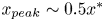 $x_{peak}\sim 0.5 x^*$. As evidenced in Cafiero et al. (Reference Cafiero, Discetti and Astarita2015), the growing shear layer determines an asymmetric spreading of the wakes generated by the grid bars, with a larger value of the spreading rate towards the centreline. This effectively causes an upstream shift of the location where the wakes meet, hence resulting in an upstream shift of the peak in the turbulence intensity profile. Considering the location of the local maxima, i.e. the first peak in the streamwise velocity fluctuation profile, obtained for the four investigated FGs, figure 9 shows the scaling as a function of
  $x^*$. It is interesting to see that there is still a clear correlation with the wake interaction length scale. Nevertheless, a significant upstream shift of the peak with respect to the grid turbulence case can be detected. This difference must be attributed to the effect of the growing shear layers, which causes a higher spreading rate of the wakes shed from the grid bars, and the consequent shift of
  $x_{peak}$.

Figure 9. Location of the maximum in the  $u^{\prime }/U_b$ profiles for the four investigated FGs,
  $x_{peak}$, as a function of the wake interaction length scale
  $x^*$. Data are normalized with respect to the jet diameter
  $D$.
$D$.
The radial velocity fluctuations show a similar trend both in terms of the location of the peak ( $x_{peak}$) and in terms of the local maximum, with the FG2 case being the largest.
For  $x>x_{peak}$, the velocity fluctuations do not decay monotonically because of the development of the external shear layer, such that a second turbulence production region is visible. Figure 7 shows that the axial location at which the shear layer turbulence production overcomes the grid turbulence decay depends on
  $t_r$, so that lower
  $t_r$ values cause an upstream shift of this position. Moreover, for fixed values of
  $N$, whilst the radial fluctuation profiles almost collapse for
  $x/D>5$, significant differences can be observed in the axial fluctuations curves: the FG4 curve shows an absolute maximum of
  $u^{\prime }/U_b$ at about
  $x/D=6$ which is 15 % larger than the corresponding peak relative to FG1. It is also relevant to point out that the location of the maximum r.m.s. of the axial and radial velocity fluctuations is not affected by
  $N$ and
  $t_r$, showing that it is fundamentally regulated by the location where the jet shear layer meets at the centreline. The difference in the intensity values does not show any clear trend with
  $t_r$. Furthermore, the significantly lower intensity obtained in the SG1 and SG2 cases compared to FG2 can be attributed to the lower value of the grid blockage ratio.
Finally, figure 7 also shows the  $u^{\prime }/U_b$ and the
  $v^{\prime }/U_b$ profiles related to the RG. As can be seen, the strong peak of the velocity fluctuations produced in this case featured at about
  $x/D=0.18$ (i.e.
 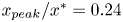 $x_{peak}/x^*=0.24$) rapidly decays, following the power law which is expected for RG-generated turbulence (Comte-Bellot & Corrsin Reference Comte-Bellot and Corrsin1966). Even in this case a second region of turbulence production is detected for
  $x/D>3$ where, opposite to the FG and the SG cases, the profiles collapse with the JWT ones, thus suggesting most of the turbulence produced by the grid has already been dissipated. It is worth noticing that the use of the RG is advantageous, in terms of turbulence production, up to 1.4
 $D$ with respect to the SGs and up to 1.3
 $D$ with respect to FG4, a value that goes down to 0.9
 $D$ for FG1.
3.2. One-point turbulent kinetic energy equation
We now turn to the estimates of the main terms of the single-point turbulent kinetic energy equation. The purpose of this is twofold: we are interested in highlighting firstly the effect of the secondary grid iterations on the distribution of turbulence production, dissipation and transport and secondly the effect of the grid thickness ratio on how turbulence is produced, transported and dissipated. The single-point turbulent kinetic energy equation can be expressed using a compact notation as (Valente & Vassilicos Reference Valente and Vassilicos2014)
 \begin{equation} \underbrace{\frac{\bar{U}_k}{2}\frac{\partial \overline{q^2}}{\partial x_k}}_{\mathcal{A}} = \underbrace{-\overline{u_i^{\prime} u_j^{\prime}}\frac{\partial \bar{U}_i}{\partial x_j}}_{\mathcal{P}}- \underbrace{\frac{\partial}{\partial x_k} \left( \frac{\overline{u^{\prime}_k q^2}}{2}+\frac{\overline{u^{\prime}_k p}}{\rho} \right)}_{\mathcal{T}} + \underbrace{\frac{\nu}{2}\frac{\partial^2 \overline{q^2}}{\partial x_m^2}}_{\mathcal{D}_v}-{\varepsilon}, \end{equation}
with  $q^2={u^{\prime }_i}^2$;
  $\mathcal {A}$,
  $\mathcal {P}$ and
  $\mathcal {T}$ indicate the advection, production and transport of turbulent kinetic energy, while
  $\mathcal {D}_v$ and
  $\varepsilon$ indicate the viscous diffusion and the dissipation due to the fluctuating rate of strain. For the present case, given the value of the Reynolds number,
  $\mathcal {D}_v$ is deemed to be negligible with respect to
  $\varepsilon$. The turbulent transport
  $\mathcal {T}$ is constituted by the triple velocity correlation
  $\overline {u^{\prime }_k q^2}$ and by the pressure velocity correlation
  $\overline {u^{\prime }_k p}$, which cannot be measured with the current PIV set-up. We neglect the latter term in our computation of the turbulent transport, effectively referring to the triple velocity correlation term only, and henceforth we refer to it as
 \begin{equation} \mathcal{T} = \frac{\partial}{\partial x_k} \left(\frac{\overline{u^{\prime}_k q^2}}{2}\right). \end{equation}
 One of the main issues in measurements of the turbulent dissipation is related to spatial resolution. It is indeed necessary to cope with the necessity of resolving the spatial derivatives of the velocity fluctuations, which are used to calculate the fluctuating strain rate tensor. Numerical simulations carried out to appropriately select the spatial resolution for turbulent dissipation measurements have shown that the minimum requirement for accurate sampling of the Kolmogorov length scale is in the range  $5\eta$–
 $7\eta$ (Laizet, Nedić & Vassilicos Reference Laizet, Nedić and Vassilicos2015). For the present set of experiments, in the worst-case scenario, which is attained in the wake generated by central grid item where the value of dissipation is the highest, the resolution at which we manage to resolve the velocity gradients is estimated to be
  $7\eta$. Even though this might be reflected in slightly underestimated values of the turbulent dissipation, we are mostly interested in the comparison between the different grids as a function of the thickness ratio and the number of iterations. Similarly to what was done by Li, Chen & Katz (Reference Li, Chen and Katz2017) in the case of a study of the tip gap ratio in rotating machines, we consider
  $\varepsilon$ as a pseudo-dissipation, which delivers relevant information in terms of a comparative analysis between the grids.
Further information about the assumptions made to measure each term of (3.1) is reported in Appendix A.
Figure 10 shows the production ( $\mathcal {P}$), dissipation (
 $\varepsilon$) and transport (
 $\mathcal {T}$) terms for the SG1 and FG2 cases. These quantities are normalized with respect to
  $U_b^3/D$. Three different streamwise locations are considered,
  $x/x^*=0.1$,
  $x/x^*=0.24$ and
  $x/x^*=0.5$, which correspond to locations in the production, peak and decay region of the turbulent velocity fluctuations (see also figure 7).

Figure 10. Production, dissipation and transport terms in the turbulent kinetic energy (3.1) for the fractal FG2 and single square SG1 grids. Data are measured at (a)  $x/x^*=0.1$, (b)
  $x/x^*=0.24$, i.e. corresponding to the peak of turbulent kinetic energy, and (c)
  $x/x^*=0.5$. Data are normalized with respect to
  $U_b^3/D$.
The two grids considered here differ in the number of iterations, while the size of the central grid item is the same. As already mentioned, this implies that the blockage ratio is significantly different. This comparison is helpful in assessing how the presence of the secondary grid iterations alters the production, transport and dissipation profiles.
In the production region ( $x/x^*=0.1$), a first difference between the two grids is related to the significantly larger values of production for the FG2 case. This difference can be attributed to the larger value of the blockage ratio of the FG2 case. Interestingly, the overall behaviour of the profiles is unmodified. It is reasonable to assume that the effect of the secondary iterations becomes more relevant at larger distances, where their wakes meet at the centreline. This is indeed the case near the peak of the turbulence intensity, where the profiles obtained with FG2 and SG1 show a different behaviour (figure 10b). However, the presence of the second and third iterations reflects a significantly higher production
  $\mathcal {P}$ across the whole jet width, with intense peaks also in the external shear layer region (
 $y/D=\pm 0.5$). The intense activity occurring in the external shear layer can be related to the observations of Cafiero et al. (Reference Cafiero, Discetti and Astarita2015): they observed that FGs significantly enhance the entrainment rate of the jet, with higher values of the Reynolds shear stress
  $\overline {uv}$. Later in the paper, for the FG2 case will be shown the existence of a correlation between the structures produced past the grid and those generated within the jet shear layer, which is most likely responsible for the strong peaks in the turbulence production.
The dissipation profiles show a more clear dependence on the grid geometry. Large dissipation values can be detected in the jet shear layer ( $y/D=\pm 0.5$) and in the lee of the central grid bar item (
 $y/D=\pm 0.25$). However, the FG2 case also shows two inner peaks, which are likely to be attributable to the grid geometry and, more specifically, to the secondary grid iterations.
The most prominent differences between the two cases are related to the turbulent transport. At the centreline, both cases feature values of transport equal to zero. Both the terms  $\overline {q^2u^{\prime }}$ and
  $\overline {q^2v^{\prime }}$ are indeed close to zero:
  $\overline {q^2v^{\prime }}$ from symmetry arguments, while at small distances from the grid, the streamwise velocity fluctuations are still quite small, leading to
  $\overline {q^2u^{\prime }}\approx 0$.
As  $|y/D|$ increases, for the SG1 case the wake-like behaviour is reflected in alternating positive–negative values of the transport. The spreading wake produced by the central grid item is characterized by positive values of
  $\mathcal {T}$; conversely, at
  $y/D=\pm 0.25$ a strong negative peak is related to the negative streamwise velocity fluctuations produced by the grid item, locally acting as a bluff body.
The same profile shows a much more complex behaviour in the FG2 case, which is likely to be attributable to the grid geometry. Particularly interesting are the differences between the two cases near the interface between the jet core and the surrounding ambient. The FG2 case shows local peaks of turbulent transport, which are likely to be related to the higher entrainment rate that characterizes the FGs (Cafiero et al. Reference Cafiero, Discetti and Astarita2015).
The same comparison is also carried out at larger distances from the grid exit section. At  $x/x^*=0.24$, the turbulent production
  $\mathcal {P}$ is mostly related to the jet shear layer for the SG1 case. On the other hand, the FG2 case still shows large values of production in the lee of the grid items. As expected by inspection of (3.1), the leading production term is
  $\overline {u^{\prime }v^{\prime }}({\partial \bar {U}}/{\partial y})$, which is zero from symmetry arguments. At the centreline, the term
  $\overline {{u^{\prime }}^2}({\partial \bar {U}}/{\partial x})$ is not zero, indeed being the relevant production term, it is still significantly smaller than the values elsewhere across the jet. It is also relevant to point out that the term
  $\overline {u^{\prime }w^{\prime }}({\partial \bar {U}}/{\partial z})$ is also zero in the investigated plane, as
  ${\partial \bar {U}}/{{\partial z}}$ is zero from symmetry arguments.
The large values of streamwise and lateral velocity fluctuations are then associated with the turbulent transport that takes place from wake regions towards the jet centreline. Figure 10(b) indeed shows that the turbulent transport at the centreline is larger for the FG2 case; at the same time, the dissipation values for the two cases are not dissimilar, hence justifying the higher values of velocity fluctuations for FG2.
The differences between the two grids become less relevant at larger streamwise distances. At  $x/x^*=0.5$, the FG2 case features values of production and transport larger than those for SG1 near the flow boundaries. At the centreline, the dissipation values overcome turbulent transport, with corresponding decay of the velocity fluctuations (figure 7).
The effect of the grid geometry is also assessed looking at the results obtained from the four different FGs. The FG2 grid data are replotted in figure 11 to allow an easier comparison. A first immediate observation is that the thickness ratio has a direct impact on the  $\mathcal {P}, \mathcal {T}$ and
  $\varepsilon$ profiles. Larger values of production, dissipation and transport can be detected as
  $t_r$ increases, particularly near the grid (figure 11a). The FG1 and FG2 cases are characterized by larger values of the central grid item thickness
  $t_0$, with correspondingly higher lateral mean flow shear rates. This leads to the progressively larger values of production evidenced in figure 11.

Figure 11. Production, dissipation and transport terms in the turbulent kinetic energy (3.1) for the four investigated FGs. Data are measured at (a)  $x/x^*=0.1$, (b)
  $x/x^*=0.24$, i.e. corresponding to the peak of turbulent kinetic energy, and (c)
  $x/x^*=0.5$. Data are normalized with respect to
  $U_b^3/D$.
As the distance from the grid increases (figure 11b,c), the production, dissipation and transport profiles still show a clear trend as a function of  $t_r$. It is also interesting to notice that the FG1 and FG2 cases, which are characterized by the largest value of
  $t_r$, display significantly larger peaks in both
  $\mathcal {P}$ and
  $\mathcal {T}$, whilst the FG3 and FG4 cases are closer to the SG case.
3.3. Flow-field reconstruction using proper orthogonal decomposition
The introduction of multiple scales significantly increases the complexity of the flow field. In particular, the FG geometry gives rise to a wealth of structures that pose a serious problem for their detection. With the aim of characterizing the near-field topology in the presence of a FG, we use proper orthogonal decomposition (POD) to identify the energy-containing modes of the flow. We implement the POD algorithm as proposed by Sirovich (Reference Sirovich1987), which is particularly suitable for PIV data. The velocity field  ${\boldsymbol{\mathsf{U}}}$ can be decomposed as:
 \begin{equation} {\boldsymbol{\mathsf{U}}} = {\boldsymbol{\varPsi}} \, {\boldsymbol{\varSigma}}\, {\boldsymbol{\varPhi}},\end{equation}
where  ${\boldsymbol {\varPsi }}$ and
  ${\boldsymbol {\varPhi }}$ represent the decomposition basis of the velocity field
  ${\boldsymbol{\mathsf{U}}}$, respectively, in time and space and
  ${\boldsymbol {\varSigma }}$ is the diagonal matrix containing the singular values of the velocity field. The velocity field can be decomposed into a number of modes equal to the number of snapshots. As suggested by Raiola, Discetti & Ianiro (Reference Raiola, Discetti and Ianiro2015), it is possible to operate a low-order reconstruction of the velocity field, where only a subset of modes are considered. The choice of the number of modes can be dictated by energy considerations, such as only a given share of the total amount of energy is kept within the reconstructed field. With
  $k$ being the total number of modes that are deemed sufficient to reconstruct the velocity field, one obtains
 \begin{equation} {\boldsymbol{\mathsf{U}}}_{k} = {\boldsymbol{\varPsi}} \, {\boldsymbol{\mathsf{I}}}_{k} \, {\boldsymbol{\varSigma}}\, {\boldsymbol{\varPhi}} = {\boldsymbol{\varPsi}} \, {\boldsymbol{\mathsf{I}}}_{k} \, {\boldsymbol{\varPsi}}^T {\boldsymbol{\mathsf{U}}}, \end{equation}
where  ${\boldsymbol{\mathsf{I}}}_{k}$ is a diagonal square matrix of size equal to the number of snapshots with only the first
  $k$ diagonal elements equal to 1 and 0 elsewhere (the resulting rank of
  ${\boldsymbol{\mathsf{I}}}_{k}$ is
  $k$). We perform the POD analysis for three representative cases, JWT, FG2 and SG1, and use it to evidence the flow structure considering only those modes that carry the highest share of energy. The POD analysis is performed on the instantaneous flow fields measured in the
  $xy$ plane (i.e. along the
  $0^{\circ }$ direction). In this sense, POD can be particularly instrumental in performing a comparative analysis between different inflow conditions (Taira et al. Reference Taira, Hemati, Brunton, Sun, Duraisamy, Bagheri, Dawson and Yeh2019).
With the aim of understanding the interaction between the structures produced by the grid and the external shear layer, we look at the flow field reconstructed considering only the first 10 POD modes. The relatively low number of modes is chosen to highlight the effect of the large structures produced by the presence of the grid and their interaction with the growing shear layer. The number of modes being fixed, this corresponds to different values of total energy, ranging from 15 % for the FG2 case to 20 % for the SG1 case and 35 % for the JWT case. We compared the reconstructed field obtained keeping the number of modes fixed with the case where the modal energy was considered as fixed and equal to 20 %, without noticing significant differences.
Figure 12(a) shows the contour representation of the instantaneous out-of-plane fluctuating vorticity component  $\omega _z D/U_b$ with overlaid streamlines in the JWT (top), FG2 (middle) and SG1 (bottom) cases. The JWT case evidences the presence of large coherent structures originating in the jet shear layer. These structures arise as a consequence of the Kelvin–Helmholtz instabilities at short distances from the nozzle exit section. The jet core features vorticity values close to zero, the jet still being in the potential core region.

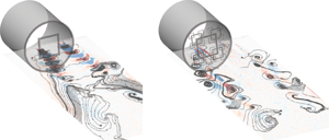
Figure 12. (a) Contour representation of the instantaneous out-of-plane fluctuating vorticity component  $\omega _z D/U_b$ with overlaid streamlines. Three different inlet conditions are considered: JWT, FG2 and SG1. The instantaneous realization is obtained as a low-order reconstruction considering only the first 10 most energetic modes. (b) Schematic description of the inward and outward spreading wake.
The FG2 case exhibits a marked change in the vorticity field structure that can be easily seen from visual inspection. A more detailed analysis of the instantaneous vorticity field reveals a complex evolution of the flow structures in the near field of the jet. For the sake of explanation, it is convenient to define as the inward spreading wake the portion of the wake produced by the grid bar item which is directed towards the jet axis, whilst as the outward spreading wake the portion of the wake that evolves towards the outer shear layer. A schematic description is provided in figure 12(b). Even though the two wake regions are originated by the same grid item, their evolution and the structures thereby produced are significantly different. The inward spreading wake is characterized by small-scale structures, that merge at  $x/D\approx 1.4$. This result is consistent with the location of the maximum in the r.m.s. of the streamwise velocity component. Conversely, the outward spreading portion of the wake shows a growth of the coherent structures as a consequence of the interaction with the structures produced in the external shear layer.
The SG1 case features alternate patches of positive and negative vorticity produced in the lee of the grid item, which can be attributed to the typical Karman wake. Interestingly, despite the same geometry of the grid item, the fractal geometry has a marked impact on the vorticity field. The effect of the second iterations is indeed such that the large coherent structures shed by the grid item are replaced by more turbulent smaller eddies. Furthermore, the effect is also reflected in the external shear layer. In the SG1 case, the large rollers produced in the shear layer are not detected. This difference has a strong impact on the entrainment rate of the jet (Cafiero et al. Reference Cafiero, Discetti and Astarita2015) as well as the turbulence production evidenced in figure 10.
This aspect has been already investigated in the case of freely decaying turbulence by Melina, Bruce & Vassilicos (Reference Melina, Bruce and Vassilicos2016). Even though the inlet conditions are similar, it must be pointed out that the present case of turbulent jet is characterized by the additional effect of the spreading shear layer, which eventually interacts with the structures shed by the grid items. In that case, the authors compared the effects of a square FG to a single square having the same blockage ratio and showed that the fractal geometry is responsible for the suppression of vortex shedding. A similar result is reported in figure 13, where the spectra of the lateral velocity component  $E_v$ obtained in the FG2 and SG1 cases are plotted as a function of
  $k t_0$, where
  $k$ is the wavenumber and
  $t_0$ the thickness of the central grid item. The spectra are obtained considering the lateral velocity component measured at
  $y/D=0.25$ (i.e. in the lee of the central grid item). The clear peak observed at
  $k t_0=0.15$ and associated with the vortex shedding in the SG1 case disappears in the FG2 case.

Figure 13. Pre-multiplied spectra of the lateral velocity component  $k^{5/3}E_v$ calculated at
  $y/D=0.25$ for the SG1 and FG2 cases.
Besides providing a qualitative description of the flow field, we further investigate the correlation between the structures produced within the external shear layer and those shed by the interaction of the mean flow with the grid bars. Figure 14(a) shows the cross-correlation ( $R_{V_{w}-V_{sl}}$) between the lateral velocity component measured at
  $y/D=0.25$,
  $V_w$, and the lateral velocity component measured at the shear layer,
  $V_{sl}$; we define this location as the value of
  $y/D$ such that
  $\bar {U}/U_c=0.5$, with
  $U_c$ being the value of the mean streamwise velocity component at the centreline (
 $y/D=0$). The FG2 case shows an extremely clear alternating behaviour, with a peak-to-peak distance equal to
  $D$. The SG1 case, on the other hand, features a significantly smaller correlation, thus confirming the observation raised from the analysis of the instantaneous reconstructed flow field.

Figure 14. (a) Cross-correlation of the lateral velocity measured at  $y/D=0.25$ with the lateral velocity measured at the jet shear layer for the SG1 and FG2 cases. (b) Cross-correlation of the lateral velocity measured at
  $y/D=0.25$ with the lateral velocity measured at
  $y/D=-0.25$ for the SG1 and FG2 cases.
Similarly, the cross-correlation ( $R_{V_{w}-V_{w1}}$) of the lateral velocity components measured at
  $y/D=\pm 0.25$ (
 $V_w$ and
  $V_{w1}$, respectively) shows an alternating behaviour, with a similar spatial frequency of
  $D$. The substantial difference between the SG1 and the FG2 cases might be attributed to the space-scale unfolding mechanism described by Laizet & Vassilicos (Reference Laizet and Vassilicos2012). The smaller eddies shed by the secondary grid iterations generate a cross-talk between the wakes generated at
  $y/D=\pm 0.25$, effectively being responsible for the higher values of correlation observed in figure 14(b).
4. Conclusions
The grid geometry plays a role in the location of the peak in the turbulence intensity profile. The result, previously found in decaying turbulence experiments, is confirmed in the case of submerged jets. A significant difference arises, however: the growing shear layer embedding the jet core causes an upward shift of the peak in the turbulence intensity. We demonstrate that, even with this difference, the location of the peak is still related to the grid geometry, which can be determined as a fraction of the wake interaction length scale as  $x^*=L_0^2/t_0$.
The distribution of the grid blockage ratio plays also a major role in the way turbulence is produced and dissipated; a less relevant effect is evidenced on transport. Larger thickness ratios lead to significantly larger values of production and dissipation. The overall balance is such that the turbulent kinetic energy grows with the thickness ratio, with a primary effect on the streamwise component. Nevertheless, this growth resembles the behaviour already evidenced in the convective heat transfer rate results of Cafiero et al. (Reference Cafiero, Castrillo, Greco and Astarita2017), relative to the centreline values of the Nusselt number, with an optimum value of thickness ratio of around 4. The limited number of grids do not allow for a thorough assessment of this maximum, but the agreement between the flow-field measurements and the convective heat transfer results clearly suggests that this is the case.
Furthermore, the central grid element alone is not responsible for the larger production rate experienced in FGs. The comparison with an isolated square item with the same geometry but significantly lower blockage ratio shows a marked change in the terms of the turbulent kinetic energy equation. Particularly interesting is the effect of the grid on the turbulence produced in the external shear layer, suggesting that the interaction mechanism occurring between the merging wakes plays a major role. Nevertheless, the substantial difference in the blockage ratio between the two cases does not allow any conclusion on the turbulence intensity levels attained with single SGs and FGs.
Fractal grids promote a suppression of the shedding associated with the central grid item, as demonstrated by inspection of the lateral velocity spectra. This topic has been already investigated in the literature by Melina et al. (Reference Melina, Bruce and Vassilicos2016) in the case of grid turbulence. We confirm a similar behaviour in the case of a turbulent round jet, where there is the added twist of the spreading shear layer interacting with the grid-generated structures.
The reconstructed flow field based on the leading POD modes shows significant differences in the flow structure in the lee of the isolated SG element and the FG. In particular, the SG1 case features little interaction between the structures produced by the grid item and the external shear layer, resulting in a significantly smaller production and entrainment rates.
Consistent with the multiscale geometry, FGs produce structures at multiple scales: smaller eddies in the inward spreading wake, whose interaction leads to large values of turbulence intensity obtained in the FG case; larger structures which interact at the flow boundaries and that can be attributed to the enhanced entrainment rate of FGs (compared with the JWT). The comparison with the single SG (with smaller value of thickness ratio) allows us to determine that the effect of the secondary grid iterations is mostly limited to the turbulence transport. This behaviour is also reflected in the results obtained in the previous section of the paper, where we see a strong correlation between the lateral velocity signal measured at  $y/D=0.25$ and the values obtained both in the jet shear layer and at
  $y/D=-0.25$. This result provides the first experimental evidence of the space-scale unfolding mechanism discussed by Laizet & Vassilicos (Reference Laizet and Vassilicos2012), who showed that FGs can deliver substantially larger values of scalar transfer and turbulent diffusion due to the multiscale nature of the generated turbulent field. The authors supported this statement showing temperature–velocity correlations in the case of grid turbulence. We show that, despite suppressing vortex shedding, the effect of the FG is such to produce a multiscale turbulent flow with an enhanced correlation between the structures produced by the central grid item and those in the jet shear layer, effectively suggesting an enhanced turbulence transport across the jet.
Declaration of interest
The authors report no conflict of interest.
Appendix A
In this appendix we detail the assumptions made to calculate the terms of (3.1). Given the nature of the PIV measurement technique, we have only access to the in-plane components ( $x,y$) of the velocity vector and its in-plane spatial derivatives.
The dissipation ( $\varepsilon$) is defined as
 \begin{equation} \varepsilon=2 \nu \overline{s_{ij}s_{ij}}, \end{equation}
with  $s_{ij}=\partial u'_i/\partial x_j$ being the fluctuating velocity strain rate tensor components. Given the limitations of our PIV set-up, we are limited to the in-plane velocity components and derivatives, such that
  $s_{ij}=\partial u'/\partial y + \partial v'/\partial x$.
The production term is defined as
 \begin{equation} \mathcal{P}={-}\overline{u'_i u'_j}\partial \bar{U}_i/\partial x_j. \end{equation}
In the present case, we measure it as  $\mathcal {P}=-\overline {u'^2}\partial \bar {U}/\partial x -\overline {u' v'}\partial \bar {U}/\partial y$, with the second term being a leading term anywhere across the jet, apart from the centreline (where
  $\partial \bar {U}/\partial y=0$).
Lastly, the turbulence transport is defined as
 \begin{equation} \mathcal{T}=\frac{\partial}{\partial x_k}\left( \frac{\overline{u^{\prime}_k q^2}}{2}+\frac{\overline{u^{\prime}_k p}}{\rho} \right). \end{equation}
Given the limitations of the temporal resolution of the PIV system and since we do not have access to any pointwise fluctuating pressure measurements, we cannot measure the pressure–velocity correlation terms in the computation of the turbulence transport. Hence, we can only estimate the transport associated with the triple velocity correlation, as  $\mathcal {T}=({\partial }/{\partial x})(\overline {u'q^2}/2)+({\partial }/{\partial y})(\overline {v'q^2}/2)$.


 Open access