


1. Introduction
In magnetised fluids of large but finite conductivity, tearing-type instabilities frequently arise in regions where one component of the magnetic field changes sign. In such regions field lines can easily reconnect, forming structures of closed field lines known as plasmoids or ‘magnetic islands’ (Ji et al. Reference Ji, Daughton, Jara-Almonte, Le, Stanier and Yoo2022). Tearing instabilities have long been studied in the context of plasma confinement experiments (Furth, Killeen & Rosenbluth Reference Furth, Killeen and Rosenbluth1963), the Earth's magnetotail (Coppi, Laval & Pellat Reference Coppi, Laval and Pellat1966) and the solar atmosphere (Somov & Verneta Reference Somov and Verneta1993), and more recently in diverse areas such as neutron stars (Lyutikov Reference Lyutikov2003; Wood, Hollerbach & Lyutikov Reference Wood, Hollerbach and Lyutikov2014; Gourgouliatos & Hollerbach Reference Gourgouliatos and Hollerbach2016), post-main-sequence stars (Kaufman et al. Reference Kaufman, Lecoanet, Anders, Brown, Vasil, Oishi and Burns2022) and generic magnetohydrodynamic (MHD) turbulence (Boldyrev & Loureiro Reference Boldyrev and Loureiro2018). In each of these contexts, the crucial property of the instability is that it leads to reconnection, releasing energy from the magnetic field, even in fluids that are close to the ideal MHD limit.
The simplest geometry in which to study tearing instability is the ‘sheet pinch’ (Furth et al. Reference Furth, Killeen and Rosenbluth1963), in which a thin and flat current sheet is embedded within a large-scale magnetic field. Furth et al. (Reference Furth, Killeen and Rosenbluth1963) considered an MHD model with asymptotically small resistivity, and showed that the tearing instability can be described analytically by solving the ideal equations in the bulk of the fluid, solving the resistive equations in a boundary layer within the current sheet and asymptotically matching these solutions. Their model included variations in density and resistivity, but to simplify the analysis they assumed that such variations are small, and they made a further approximation that is valid only if the growth rate is slower than resistive diffusion across the boundary layer; this latter approximation came to be known as the ‘constant- $\psi$ approximation’. Later studies have generalised this analysis to include various additional physical effects, but the majority of analytical results to date have been dependent on the same constant- $\psi$ approximation. Under this approximation, the existence of the instability can be demonstrated, but it is not possible to obtain the full dispersion relation or to identify the fastest growing mode. An alternative approach is to solve the full set of (linear or nonlinear) equations numerically (e.g. Dahlburg et al. Reference Dahlburg, Zang, Montgomery and Hussaini1983; Califano et al. Reference Califano, Prandi, Pegoraro and Bulanov1999; Attico, Califano & Pegoraro Reference Attico, Califano and Pegoraro2000; Landi et al. Reference Landi, Londrillo, Velli and Bettarini2008; Jelínek et al. Reference Jelínek, Karlický, Van Doorsselaere and Bárta2017; Kaufman et al. Reference Kaufman, Lecoanet, Anders, Brown, Vasil, Oishi and Burns2022). However, with this approach it is not possible to understand how the instability behaves in the asymptotic regime of high conductivity, which is often the regime of most physical interest.
Coppi et al. (Reference Coppi, Galvao, Pellat, Rosenbluth and Rutherford1976) and Pegoraro & Schep (Reference Pegoraro and Schep1986) showed that, in the simplest case (with constant density and resistivity), the boundary-layer problem can be solved analytically, which allows the full dispersion relation to be obtained and the fastest-growing mode to be identified. In fact, this boundary-layer problem had already been solved earlier by Gibson & Kent (Reference Gibson and Kent1971), and generalised to include density stratification by Baldwin & Roberts (Reference Baldwin and Roberts1972). Unfortunately, their work seems to have been largely overlooked in the plasma physics community, and the full solution of the unstratified case is usually attributed to Coppi et al. (Reference Coppi, Galvao, Pellat, Rosenbluth and Rutherford1976) (e.g. Boldyrev & Loureiro Reference Boldyrev and Loureiro2018).
In early studies, density stratification was often included because of its analogy with the effect of stellarator curvature (e.g. Furth et al. Reference Furth, Killeen and Rosenbluth1963; Johnson, Greene & Coppi Reference Johnson, Greene and Coppi1963). In the present work, our motivation is the solar tachocline, which is a strongly stably stratified layer within the Sun that is believed to harbour a strong toroidal magnetic field. There are many instabilities that may play a role in the dynamics of the tachocline, such as magnetic buoyancy (Parker Reference Parker1955; Hughes Reference Hughes, Hughes, Rosner and Weiss2007; Gilman Reference Gilman2018), magneto-rotational instability (Balbus & Hawley Reference Balbus and Hawley1991; Ogilvie Reference Ogilvie, Hughes, Rosner and Weiss2007; Parfrey & Menou Reference Parfrey and Menou2007; Kagan & Wheeler Reference Kagan and Wheeler2014; Gilman Reference Gilman2018), clamshell and tipping-type instabilities (Cally, Dikpati & Gilman Reference Cally, Dikpati and Gilman2003), as well as non-magnetic, shear-driven instabilities (Spiegel & Zahn Reference Spiegel and Zahn1970; Garaud Reference Garaud2001). However, the possibility of tearing instability has seldom been mentioned in this context, outside of a few studies (Ji & Daughton Reference Ji and Daughton2011; Lewis Reference Lewis2022), none of which considered the effect of stratification. Recently, however, it has been suggested that the tachocline contains a toroidal field whose sign oscillates in the radial direction, as a result of inward diffusion of the cyclic dynamo field from the overlying convective envelope (Forgács-Dajka & Petrovay Reference Forgács-Dajka and Petrovay2001; Barnabé et al. Reference Barnabé, Strugarek, Charbonneau, Brun and Zahn2017). Whether such a field configuration is compatible with the Sun's interior rotation, and with the solar dynamo cycle, remains a matter of debate (e.g. Gough Reference Gough, Hughes, Rosner and Weiss2007; Matilsky et al. Reference Matilsky, Hindman, Featherstone, Blume and Toomre2022). In any case, such a field configuration seems likely to be subject to tearing instability, unless it is suppressed by the tachocline's stabilising stratification. This motivates us to investigate the degree to which stable stratification affects the instability, and hence to assess whether it can arise within the solar tachocline.
In this paper we re-derive the boundary-layer solution of Baldwin & Roberts (Reference Baldwin and Roberts1972) and use it to fully describe the effect of stratification on the tearing instability. We identify several different parameter regimes depending on the degree of stratification, and demonstrate that previous results are reproduced in particular asymptotic limits. We then confirm our results by solving the linearised equations numerically. The plan of the paper is as follows. Our mathematical model is defined and the equations are linearised in § 2. We derive analytical solutions valid in the bulk and boundary layer in §§ 3 and 4, respectively. In § 5 we use asymptotic matching to obtain an implicit dispersion relation, and describe its properties in the asymptotic limit of large conductivity. In § 6 we solve the linearised equations numerically, validating the analytical results and quantifying the effect of finite conductivity and domain size on the instability. The results are applied to the solar tachocline in § 7, where we also consider the effect of thermal diffusion. We summarise our findings in § 8.
2. The sheet pinch model
We consider an inviscid, stably stratified, Boussinesq fluid under the MHD approximation:
 $$\begin{gather} \frac{\partial\boldsymbol{u}}{\partial t} + \boldsymbol{u}\boldsymbol{\cdot} \boldsymbol{\nabla} \boldsymbol{u} =-\frac{1}{\rho_0}\boldsymbol{\nabla} P + \theta\boldsymbol{e}_{z} + \frac{1}{4{\rm \pi}\rho_{0}}(\boldsymbol{\nabla} \times \boldsymbol{B})\times\boldsymbol{B}, \end{gather}$$
 $$\begin{gather}\frac{\partial\boldsymbol{B}}{\partial t} = \boldsymbol{\nabla} \times(\boldsymbol{u} \times\boldsymbol{B}) + \eta\nabla^{2}\boldsymbol{B}, \end{gather}$$
 $$\begin{gather}\boldsymbol{\nabla} \boldsymbol{\cdot} \boldsymbol{B} = 0, \end{gather}$$
 $$\begin{gather}\boldsymbol{\nabla} \boldsymbol{\cdot} \boldsymbol{u} = 0, \end{gather}$$
 $$\begin{gather}\frac{\partial\theta}{\partial t} + \boldsymbol{u} \boldsymbol{\cdot} \boldsymbol{\nabla} \theta =-N^{2}u_{z}, \end{gather}$$
where  $\boldsymbol {e}_{z}$ is the unit vector in the $z$ (vertical) direction, $P$ is the pressure, $\rho _0$ is the (constant) reference density, $\boldsymbol {u}$ is the fluid velocity, with vertical component $u_z$, $\boldsymbol {B}$ is the magnetic field (measured in Gaussian c.g.s. units), $\eta$ is the magnetic diffusivity, $N$ is the (constant) buoyancy frequency and $\theta$ is the buoyancy variable.
In these equations we have included magnetic diffusion, because it is essential for tearing instability to operate, but we have neglected the diffusion of both momentum and temperature. As we shall see, this simplification makes it possible to solve the boundary-layer problem analytically. The effect of momentum diffusion is generally to reduce the growth rate, as has been demonstrated in previous works (e.g. Porcelli Reference Porcelli1987; Tenerani et al. Reference Tenerani, Rappazzo, Velli and Pucci2015). The effect of thermal diffusion, which is certainly important in the solar tachocline, is addressed in § 7.1. Unsurprisingly, the main consequence of including thermal diffusion is to reduce the stabilising effect of the stratification.
2.1. Background state
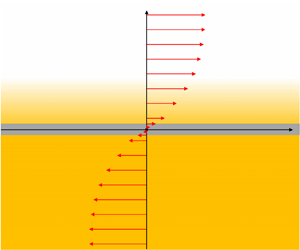
As illustrated in figure 1, we consider a background state at rest with a magnetic field  $\boldsymbol {B} = (B(z),0,0)$ in Cartesian coordinates. The crucial condition for tearing instability to occur is that the sign of $B(z)$ reverses for some value of $z$, which we take to be $z=0$ without loss of generality. The fastest-growing tearing modes are generally found to be invariant in the direction of the electric current (e.g. Furth et al. Reference Furth, Killeen and Rosenbluth1963), which in our case is the $y$ direction, and so for simplicity we only consider two-dimensional perturbations in the $xz$ plane. Such modes are insensitive to any component of the background field in the $y$ direction, and so we have taken this to be zero without loss of generality. For simplicity we assume that $B(z)$ is an odd function, which implies that the solutions of the linear perturbation problem have either even or odd symmetry.

Figure 1. Initial background state configuration. Horizontal arrows indicate the strength and direction of the magnetic field, and the colour gradient indicates the stable density stratification. Tearing instability arises from magnetic diffusion within an internal boundary layer, indicated by a thin grey strip around the  $x$ axis.
In what follows, for definiteness we generally adopt the so-called Harris field,
 \begin{equation} B(z) = \sqrt{4{\rm \pi}\rho_0}\beta\ell \tanh(z/\ell)\end{equation}
(named for Harris (Reference Harris1962)), where the constant  $\beta$ quantifies the Alfvénic shear in the current sheet, which has thickness $\ell$. We then define the Lundquist number as
 \begin{equation} S \equiv \frac{\beta\ell^2}{\eta}.\end{equation}
However, it is straightforward to generalise our results to other choices for the background field.
We note that the background state is not strictly a steady solution of the induction equation (2.2) in the presence of finite resistivity. However, we are concerned with the regime in which  $\eta$ is very small, in the sense that $S \gg 1$, and the slow diffusion of the background state can be neglected provided that the instability grows on a time scale much shorter than the bulk diffusion time, $\ell ^2/\eta$. In what follows, it is often convenient to measure quantities in units defined by the background field, and in particular to use $\ell$ as the length scale and $1/\beta$ as the time scale, in which case the condition for self-consistency of our instability analysis is naturally written as $\sigma /\beta \gg 1/S$, where $\sigma$ is the growth rate. In terms of these natural units, the strength of the stratification can be expressed as a ‘magnetic Richardson number’,
 \begin{equation} R_B \equiv \frac{N^2}{\beta^2}, \end{equation}
named by analogy with the hydrodynamic Richardson number that determines the stability of shear flows.
2.2. Linear perturbations
As mentioned above, we anticipate that the fastest-growing tearing mode will be invariant in the direction of the electric current, which is the  $y$ direction for our choice of background state. We therefore consider small perturbations to the background state in the form
 \begin{equation} a(x,z,t) = \mathrm{e}^{\mathrm{i} kx + \sigma t}\hat{a}(z), \end{equation}
where  $a(x,z,t)$ represents a perturbation to any of the variables, $k$ is the wavenumber, $\sigma$ is the growth rate and $\hat {a}(z)$ is the perturbation eigenfunction. The linearised versions of (2.1)–(2.5) can then be reduced to the following pair of coupled ordinary differential equations for the $z$ components of $\boldsymbol {u}$ and $\boldsymbol {b}$:
 $$\begin{gather} \sigma^2\hat{u}_{z}'' - (\sigma^2 + N^2)k^2\hat{u}_{z} = \frac{\mathrm{i} k\sigma}{4{\rm \pi}\rho_0}[B\hat{b}_{z}'' - (k^{2} B + B'')\hat{b}_{z}], \end{gather}$$
 $$\begin{gather}\eta\hat{b}_{z}'' - (\eta k^2 + \sigma)\hat{b}_{z} =- \mathrm{i} kB\hat{u}_{z}, \end{gather}$$
where a prime ( $'$) denotes a derivative with respect to $z$.
$z$.
Following the method introduced by Furth et al. (Reference Furth, Killeen and Rosenbluth1963), we consider separately the bulk and boundary-layer regions of the domain, solving a leading-order asymptotic approximation to (2.10) and (2.11) in each region. The solutions will then be connected by asymptotic matching, in order to obtain a dispersion relation for the tearing instability. For simplicity, we take the bulk domain to be infinite in extent, with a background field  $B(z)$ that is bounded in magnitude. In that case, the only physically meaningful solutions are those for which the perturbations are also bounded at infinity, and this will serve as our boundary condition. (Other solutions would correspond to an injection of energy from infinity, rather than an instability arising internally.) Furthermore, if $B(z)$ is an odd function (as we assume throughout) then we generally expect the fastest-growing solution to have an even $\hat {b}_{z}(z)$, and therefore an odd $\hat {u}_{z}(z)$, along with a real growth rate. These properties, which are frequently assumed in studies of tearing instability (e.g. Coppi et al. Reference Coppi, Galvao, Pellat, Rosenbluth and Rutherford1976), are confirmed in Appendix A.
3. The bulk solution
Within the bulk of the domain we neglect the diffusion of the field, and therefore omit the terms in (2.11) involving  $\eta$; this approximation requires the growth rate, $\sigma$, to exceed the rate of diffusion, i.e. $\sigma \gg \eta (k^2 + 1/\ell ^2)$. Having neglected these terms, it is straightforward to combine (2.10) and (2.11) into a single equation:
 \begin{equation} \sigma^2\hat{u}_{z}'' - (\sigma^2 + N^2)k^2\hat{u}_{z} = \frac{k^2}{4{\rm \pi}\rho_0}[(B^2\hat{u}_{z}')' - k^{2}B^2 \hat{u}_{z}]. \end{equation}
We further assume that the growth rate of the instability is small compared with the Alfvén frequency, i.e.  $\sigma \ll \beta \ell k$, which allows us to neglect the terms involving $\sigma ^2$ on the left-hand side of this equation. The validity of all these assumptions will be verified once the growth rate is known. Thus, we finally arrive at the bulk equation
 \begin{equation} (B^2\hat{u}_{z}')' = (k^2B^2 + 4{\rm \pi}\rho_0 N^2)\hat{u}_{z}. \end{equation}
 The same equation was obtained by Furth et al. (Reference Furth, Killeen and Rosenbluth1963), although they assumed that the  $N^2$ term was small enough to be neglected in the bulk. When this term is not negligible, which is the regime of interest in the present work, the nature of the bulk equation changes subtly but significantly (e.g. Johnson et al. Reference Johnson, Greene and Coppi1963). We note that $z=0$, which is the location of the boundary layer, is a regular singular point of (3.2). This is expected, since it is within the boundary layer that resistivity (which we have neglected in the bulk equation) is required in order to regularise the solutions. As we approach $z=0$, where we assume that the background field is of the form $B(z) \simeq \sqrt {4{\rm \pi} \rho _0}\beta z$, the general solution of (3.2) is a superposition of two Frobenius power series with the exponents $- \frac {1}{2} \pm \sqrt {\tfrac {1}{4} + N^2/\beta ^2} = - \frac {1}{2} \pm \sqrt {\tfrac {1}{4} + R_B}$. Therefore unlike the unstratified case, in which $\hat {u}_{z}$ can be written as a series in integer powers of $z$, in the stratified problem $\hat {u}_{z}$ is a superposition of power series with generally incommensurate exponents. In particular, we can anticipate that a difficulty will arise when the stratification is increased to the critical value $R_B = 3/4$, because then the Frobenius exponents will differ by $2$, implying that logarithmic terms must appear in the solution. As we shall see, this means that the usual procedure for matching the bulk solution to the boundary-layer solution fails. We note that non-integer exponents in the solution can also result from other physical processes, such as geometric curvature (Glasser, Greene & Johnson Reference Glasser, Greene and Johnson1975) and the Hall effect (Attico et al. Reference Attico, Califano and Pegoraro2000), but the consequences for the asymptotic matching problem have not been fully recognised in the literature.
The above considerations are generic for any sensible choice of background field  $B(z)$. In the particular case of the Harris field (2.6), the bulk equation can be solved in closed form by first making the transformation $T = \tanh ^2(z/\ell )$ to put it into hypergeometric form:
 \begin{equation} \frac{\mathrm{d}^2\hat{u}_{z}}{\mathrm{d}T^2} + \left(\frac{3/2}{T} - \frac{1}{1-T}\right)\frac{\mathrm{d}\hat{u}_{z}}{\mathrm{d}T} = \frac{s^2T + (r^2-\tfrac{1}{4})(1-T)}{4T^2(1-T)^2}\hat{u}_{z}, \end{equation}
where we have introduced dimensionless parameters  $r$ and $s$, which are defined as
 \begin{equation} r \equiv \sqrt{\tfrac{1}{4} + R_B} \quad \mbox{and} \quad s \equiv \sqrt{(k\ell)^2 + R_B}. \end{equation}
 The solution that has the required boundedness as  $|z| \to \infty$ can be expressed in terms of the hypergeometric function ${_2F_1}$ as
 \begin{equation} \hat{u}_{z} = T^{-{1}/{4}+({1}/{2})r}(1-T)^{s/2} {_2F_1}(\tfrac{1}{2}r+\tfrac{1}{2}s-\tfrac{1}{4},\tfrac{1}{2}r+ \tfrac{1}{2}s+\tfrac{5}{4},s+1,1-T)\operatorname{sgn}(z),\end{equation}
where we have included a factor of  $\operatorname {sgn}(z)$ so that $\hat {u}_{z}(z)$ is an odd function, for reasons explained earlier. From here on, the strength of the stratification will generally be measured in terms of the parameter $r$ or $R_B$, rather than $N$. The unstratified case corresponds to $r=1/2$, and the critical stratification mentioned above corresponds to $r=1$. From (3.5) it can be confirmed that the bulk solution near $z=0$ has logarithmic behaviour when $r=1$ (or when $r$ is any other integer; see Appendix A).
4. The boundary-layer solution
The boundary layer is assumed to be thin, in the sense that its thickness (which is precisely defined later) is smaller than both  $\ell$ and $1/k$ by a factor of $S$ to some positive power. In (2.10) and (2.11) we therefore approximate $\nabla ^2 \simeq \partial ^2/\partial z^2$ and
 \begin{equation} B(z) \simeq \sqrt{4{\rm \pi}\rho_0}\,\beta z. \end{equation}
These approximations result in the boundary-layer equations
 $$\begin{gather} \sigma\hat{u}_{z}'' = \frac{\mathrm{i} k\beta z}{\sqrt{4{\rm \pi}\rho_0}}\hat{b}_{z}'' + \frac{k^2 N^{2}}{\sigma}\hat{u}_{z}, \end{gather}$$
 $$\begin{gather}\sigma\hat{b}_{z} = \sqrt{4{\rm \pi}\rho_0}\ \mathrm{i} k\beta z\hat{u}_{z} + \eta\hat{b}_{z}''. \end{gather}$$
Because these equations involve four derivatives, but only two factors of  $z$, they are more easily solved by working in Fourier space. Defining the Fourier transform of $\hat {u}_{z}$ as
 \begin{equation} \tilde{u}_z(\zeta) = \int_{-\infty}^{\infty}\mathrm{e}^{\mathrm{i}\zeta z}\hat{u}_{z}(z)\,\mathrm{d}z, \end{equation}
(4.2) and (4.3) can be transformed and combined into a single equation:
 \begin{equation} \left[\frac{\sigma\zeta^2}{\beta^2} + R_B\frac{k^2}{\sigma}\right]\tilde{u}_z = k^2 \frac{\mathrm{d}}{\mathrm{d}\zeta}\left(\frac{\zeta^2}{\sigma + \eta\zeta^2}\frac{\mathrm{d}\tilde{u}_z}{\mathrm{d}\zeta}\right). \end{equation}
This is a second-order ordinary differential equation in  $\zeta$, with an essential singularity at $\zeta \to \infty$. We are interested in the solution that is exponentially small at infinity, since only this solution has an inverse Fourier transform. We note that, because the function $\hat {u}_{z}(z)$ is odd, its transform $\tilde {u}_z(\zeta )$ must also be odd. We therefore solve (4.5) in the domain $0<\zeta <\infty$ and impose antisymmetry about $\zeta =0$.
As well as an essential singularity at  $\zeta \to \infty$, (4.5) also has three regular singularities at $\zeta = 0$ and at $\zeta = \pm \mathrm {i}\sqrt {\sigma /\eta }$. On closer inspection, however, the latter two are found to be only ‘apparent’ singularities, suggesting that there is a change of variable that reduces this equation to a solvable form (Shanin & Craster Reference Shanin and Craster2002). Indeed, if we define a new independent variable $X = ({\sqrt {\eta \sigma }}/{\beta k})\zeta ^{2}$ then the boundary-layer equation becomes
 \begin{equation} 4X^{1/2}\frac{\mathrm{d}}{\mathrm{d}X} \left(\frac{X^{3/2}}{X+\lambda}\frac{\mathrm{d}\tilde{u}_z}{\mathrm{d}X}\right) = \left(X + \frac{r^2-\tfrac{1}{4}}{\lambda}\right)\tilde{u}_z, \end{equation}
where  $r$ is defined as in (3.4a,b) and
 \begin{equation} \lambda \equiv \frac{\sqrt{\sigma^3/\eta}}{\beta k} = S^{1/2}(\sigma/\beta)^{3/2}(k\ell)^{-1}. \end{equation}
Following the method of Shanin & Craster (Reference Shanin and Craster2002), we can express the desired solution in terms of the Tricomi function  $U$ as
 \begin{align} \tilde{u}_z &=\mathrm{e}^{-X/2} X^{-{1}/{4}+{r}/{2}} \left[U\left(\frac{(r+\lambda)^{2}-\dfrac{1}{4}}{4\lambda},1+r,X\right)\right. \nonumber\\ &\quad +\left. \left(\frac{(\lambda-\dfrac{1}{2})^{2} - r^{2}}{4\lambda}\right) U\left(\frac{(r+\lambda)^{2}-\dfrac{1}{4}}{4\lambda} + 1,1+r,X\right)\right]\operatorname{sgn}(\zeta). \end{align}
This is equivalent to the solution obtained by Baldwin & Roberts (Reference Baldwin and Roberts1972), and in the unstratified limit,  $r\to \frac {1}{2}$, it reduces to the solution obtained by Pegoraro & Schep (Reference Pegoraro and Schep1986). From this solution, the thickness of the boundary layer can be defined as the region in which the variable $X$ is of order unity, which corresponds in $z$-space to a thickness of $(\eta \sigma )^{1/4}/(\beta k)^{1/2}$. Unfortunately, at this stage we do not know the order of magnitude of the growth rate, $\sigma$, and so the boundary layer is of indeterminate thickness. However, our earlier assumption that it is much smaller than $\ell$ can now be expressed more precisely as $\sigma /\beta \ll S(k\ell )^2$, which will be verified a posteriori.
We note, in passing, that our boundary-layer equation (4.5) has the same mathematical form as one that arises when analysing tearing instability in the electron-MHD regime (e.g. Attico et al. Reference Attico, Califano and Pegoraro2000; Wood et al. Reference Wood, Hollerbach and Lyutikov2014). However, to our knowledge, the fact that it can be solved analytically has not previously been recognised in that context.
For the purposes of asymptotically matching the boundary-layer solution to the bulk solution, as done in the following section, we need only determine the behaviour of the boundary-layer solution for ‘large’ values of  $z$ (in comparison with the scale of the boundary layer itself), which is dictated by the behaviour of (4.8) for $X \ll 1$. Specifically, we make use of the result (see Kammler Reference Kammler2008)
 \begin{equation} \tilde{u}_z(\zeta) \sim |\zeta|^{-\alpha}\operatorname{sgn}(\zeta) \ \mbox{as } \zeta\to0 \quad \Longleftrightarrow \quad \hat{u}_{z}(z) \sim \frac{|z|^{\alpha-1}\operatorname{sgn}(z)}{2\mathrm{i}\sin\left(\dfrac{\rm \pi}{2}\alpha\right)\varGamma(\alpha)} \ \mbox{as } |z|\to\infty \end{equation}
to determine the behaviour of the boundary-layer solution for large  $z$ from its solution (4.8) in Fourier space.
5. Asymptotic matching
Now that we are in possession of analytical solutions valid in the bulk and boundary-layer regions, all that is required is to asymptotically match these two solutions, and thus arrive at a dispersion relation. Following Furth et al. (Reference Furth, Killeen and Rosenbluth1963), in nearly all previous studies of tearing instability this has been achieved essentially by matching the coefficients of the two leading-order terms in the series representations for the bulk and boundary-layer solutions. Our bulk solution (3.5) for  $\hat {u}_{z}(z)$ has the form
 \begin{equation} \hat{u}_{z} = \sum_{n=0}^{\infty}[A_{n}|z|^{-{1}/{2}-r+2n} + B_{n}|z|^{-{1}/{2}+r+2n}]\operatorname{sgn}(z),\end{equation}
whereas our boundary-layer solution (4.8), after transforming back into  $z$-space, has the form
 \begin{equation} \hat{u}_{z} = \sum_{n=0}^{\infty}[a_{n}|z|^{-{1}/{2}-r-2n} + b_{n}|z|^{-{1}/{2}+r-2n}]\operatorname{sgn}(z),\end{equation}
where the coefficients  $A_n$, $B_n$, $a_n$ and $b_n$ are known functions of $k$ and $\sigma$.
Matching the first terms in each of the four series, bearing in mind that each solution also allows an arbitrary overall factor, we obtain an implicit dispersion relation:
 \begin{equation} \frac{A_{0}}{B_{0}}(k) = \frac{a_{0}}{b_{0}}(\sigma,k). \end{equation}
However, the terms that are matched under this procedure cease to be the leading-order terms when  $r \geq 1$. Indeed, if $r=1$ then, as mentioned earlier, both the bulk and the boundary-layer solutions will feature logarithmic terms (of different forms) and hence this matching process cannot be valid in that case. Fortunately, as we shall show, the tearing instability is strongly suppressed by stable stratification before this mathematical difficulty arises, so the standard matching procedure leading to (5.3) is adequate for our purposes.
Taking the values for the coefficients  $A_0$, $B_0$, $a_0$ and $b_0$ implied by (3.5) and (4.8) (see Appendix A), we thus obtain the dispersion relation
 \begin{align} &(Sk\ell)^{2r/3} \frac{\varGamma(r)}{\varGamma(-r)} \frac{\varGamma\left(\dfrac{s}{2}-\dfrac{r}{2}- \dfrac{1}{4}\right)}{\varGamma\left(\dfrac{s}{2}+\dfrac{r}{2}-\dfrac{1}{4}\right)} \frac{\varGamma\left(\dfrac{s}{2}-\dfrac{r}{2}+\dfrac{5}{4} \right)}{\varGamma\left(\dfrac{s}{2}+\dfrac{r}{2}+\dfrac{5}{4}\right)} \nonumber\\ &\quad =\lambda^{r/3} \frac{\varGamma(-r)}{\varGamma(r)}\frac{\lambda+ \dfrac{1}{2}+r}{\lambda+\dfrac{1}{2}-r} \frac{\varGamma\left(\dfrac{(\lambda+r)^2-\dfrac{1}{4}}{4\lambda} \right)}{\varGamma\left(\dfrac{(\lambda-r)^2-\dfrac{1}{4}}{4\lambda} \right)}\frac{\sin\left[\dfrac{\rm \pi}{2}\left(\dfrac{1}{2}+r\right)\right]}{\sin\left[\dfrac{\rm \pi}{2} \left(\dfrac{1}{2}-r\right)\right]}\frac{\varGamma\left(\dfrac{1}{2}+r\right)}{\varGamma \left(\dfrac{1}{2}-r\right)}. \end{align}
Although this result is highly implicit, we note that the left-hand side of (5.4) (which comes from the bulk solution) is only a function of  $k$, and the right-hand side (which comes from the boundary-layer solution) is only a function of $\lambda$, which itself is related to $\sigma$ and $k$ by (4.7). In fact, for any value of $r \in [\frac {1}{2},1)$, and for any value of $S > 0$, we can prove that there is always a single fastest-growing mode. First observe that the left-hand side of (5.4) is a positive and monotonically increasing function of $k$ for $0 < k\ell < \sqrt {r + \frac {1}{2}}$; it vanishes as $k\ell \to 0$ and diverges as $k\ell \to \sqrt {r+\frac {1}{2}}$. Meanwhile the right-hand side is a positive and monotonically decreasing function of $\lambda$ for for $0 < \lambda < r + \frac {1}{2}$; it diverges as $\lambda \to 0$ and vanishes as $\lambda \to r+\frac {1}{2}$. Therefore (5.4) describes a monotonically decreasing relation between $k$ and $\lambda$ over this range of $k$. Expressing this result in terms of the growth rate, $\sigma$, which is related to $\lambda$ by (4.7), we find that $\sigma$ vanishes at $k=0$ and at $k=\sqrt {r+\frac {1}{2}}/\ell$, and has a unique maximum within this range of $k$, which corresponds to the fastest-growing tearing mode.
In the unstratified limit,  $r \to \frac {1}{2}$, (5.4) reduces to the well-known result (e.g. Coppi et al. Reference Coppi, Galvao, Pellat, Rosenbluth and Rutherford1976; Pegoraro & Schep Reference Pegoraro and Schep1986; Boldyrev & Loureiro Reference Boldyrev and Loureiro2018)
 \begin{equation} S^{1/3}\frac{(k\ell)^{4/3}}{1-(k\ell)^2} =\frac{1-\lambda^2}{{\rm \pi}\lambda^{5/6}}\frac{\varGamma\left(\dfrac{1+ \lambda}{4}\right)}{\varGamma\left(\dfrac{3+\lambda}{4}\right)}.\end{equation}
In that case, and in the asymptotic limit  $S \to \infty$, the fastest-growing mode has $\lambda$ of order unity and $k\ell \ll 1$, such that the left-hand side can be approximated as a power law $\propto k^{4/3}$. Hence, using the definition of $\lambda$ in (4.7), the fastest-growing mode has $k\ell \sim S^{-1/4}$ and $\sigma /\beta \sim S^{-1/2}$.
Interestingly, for any non-zero amount of stratification (i.e. for any value of  $r>1/2$), the left-hand side of (5.4) has a different asymptotic behaviour in the limit $k \to 0$ (and so does the right-hand side in the limit $\lambda \to 0$). This implies that the instability changes qualitatively in the presence of stratification (at least in the asymptotic limit of large $S$), and as we show below, several distinct asymptotic regimes arise in the simultaneous limit of $S \to \infty$ and $r \to 1/2$.
Recalling the definition (3.4a,b) of  $r$ in terms of $R_B$, we note that the limit $r \to 1/2$ is equivalent to $R_B \to 0$. In the following, we therefore consider the asymptotic limit $S \to \infty$ with $R_B \sim S^{-a}$ for some positive constant $a$. To understand the behaviour of the dispersion relation (5.4) in this limit, it is helpful to consider how the left- and right-hand sides behave for different ranges of $k$ and $\lambda$, respectively. For $R_B \ll 1$, the left-hand side of (5.4) is of order
 $$\begin{gather} S^{1/3}R_B^{1/2}(k\ell)^{1/3} \quad \mbox{for } k\ell \ll R_B^{1/2}, \end{gather}$$
 $$\begin{gather}S^{1/3}(k\ell)^{4/3} \quad \mbox{for } R_B^{1/2} \ll k\ell \ll 1, \end{gather}$$
while the right-hand side is of order
 $$\begin{gather} R_B^{-1/2}\lambda^{-1/3} \quad \mbox{for } \lambda \ll R_B, \end{gather}$$
 $$\begin{gather}\lambda^{-5/6} \quad \mbox{for } R_B \ll \lambda \ll 1, \end{gather}$$
 $$\begin{gather}1 - \lambda \quad \mbox{for } \lambda \sim 1. \end{gather}$$
From this information, and the fact that  $\lambda \equiv S^{1/2}(\sigma /\beta )^{3/2}(k\ell )^{-1}$, we can identify how the growth rate, $\sigma$, scales with the wavenumber, $k$, in different regions of the parameter space. The result is shown in figure 2, which illustrates how new regimes arise as the strength of the stratification is increased (or, equivalently, as the value of the exponent $a$ is decreased). Qualitative changes to the dispersion relation occur for $a=\frac {1}{2}$, $\frac {2}{5}$, $\frac {2}{9}$ and $0$, and the form of the function $\sigma (k)$ for each of these critical values is indicated in figure 3. We note that, as we would expect in a stably stratified system, increasing the strength of the stratification acts to decrease the growth rate (at a given value of $k$).
$k$).

Figure 2. Scaling regimes, demarcated by dotted lines, for the growth rate,  $\sigma$, in the asymptotic limit $S\to \infty$. Coloured arrows track the behaviour of the fastest-growing mode as stratification is increased. The axes are logarithmic.

Figure 3. The dispersion relation in the asymptotic limit  $S \to \infty$, with $R_B \sim S^{-a}$, for $a=1/2$, $2/5$, $2/9$ and $0$. The location of the fastest-growing mode is indicated with a circle.
The assumptions made about the growth rate in §§ 3 and 4 can now be checked, with the aid of figure 2. In particular, we have assumed that  $S^{-1}(1 + (k\ell )^2) \ll \sigma /\beta \ll k\ell$ and that $\sigma /\beta \ll S(k\ell )^2$, and we find that these assumptions hold in all of the regions plotted, as long as $k\ell \gg S^{-1}$ and $R_B \ll 1$.
We are primarily interested in how the fastest-growing mode changes in the presence of stratification, and as illustrated by the dashed arrows in figure 2 there are three distinct parameter regimes to consider, which we refer to as weakly, moderately and strongly stratified.
5.1. The weakly stratified regime,  $a \geq 1/2$

If  $a > 1/2$, then in the limit $S \to \infty$ the entire dispersion relation is essentially identical to the unstratified case, $R_B=0$. The fastest-growing mode thus has $k\ell \sim S^{-1/4}$ and $\sigma /\beta \sim S^{-1/2}$, as described above.
In the case  $a=1/2$, the effects of stratification begin to affect the fastest-growing mode, and to show how we can introduce a rescaled wavenumber, $\bar {k} \equiv k\ell /R_B^{1/2}$, which remains of order unity in the limit $S \to \infty$. In this limit, the dispersion relation (5.4) can be approximated as
 \begin{equation} (SR_B^2)^{1/3}\,\bar{k}^{1/3}(1 + \bar{k}^2)^{1/2} = \frac{1-\lambda^2}{{\rm \pi}\lambda^{5/6}}\frac{\varGamma \left(\dfrac{1+ \lambda}{4}\right)}{\varGamma\left(\dfrac{3+\lambda}{4}\right)}.\end{equation}
Figure 4 illustrates how the exact dispersion relation approaches this asymptotic form for increasing values of  $S$ in the case where $R_B = 0.1S^{-1/2}$.


5.2. The moderately stratified regime, $2/9 \leq a < 1/2$

For stronger stratification (i.e. for smaller values of  $a$), the effect of stratification in the bulk domain suppresses a range of wavenumbers, including the fastest-growing mode. As a result, the fastest-growing mode shifts to smaller length scales, with $k\ell \sim R_B^{1/2}$, and has a reduced growth rate of $\sigma /\beta \sim S^{-3/5}R_B^{-1/5}$.
For  $a < 2/5$, the effects of stratification begin to be felt also in the boundary layer, suppressing very small scales, but this does not affect the fastest-growing mode until $a \leq 2/9$. In the case $a=2/9$ we can introduce rescaled parameters $\bar {k} \equiv k\ell /R_B^{1/2}$ and $\bar {\lambda } \equiv \lambda /R_B$ that remain of order unity in the limit $S \to \infty$. In this limit, the dispersion relation (5.4) can be approximated as
 \begin{equation} (SR_B^{9/2})^{1/3}\bar{k}^{1/3}(1 + \bar{k}^2)^{1/2} = \frac{1}{{\rm \pi}\bar{\lambda}^{5/6}}\frac{\varGamma \left(\dfrac{1 +1/\bar{\lambda}}{4}\right)}{\varGamma \left(\dfrac{3+1/\bar{\lambda}}{4}\right)}.\end{equation}
Figure 5 illustrates how the exact dispersion relation approaches this asymptotic form for increasing values of  $S$ in the case where $R_B = 0.1S^{-2/9}$. We note that the right-hand side of (5.9) is equivalent to the result obtained by Johnson et al. (Reference Johnson, Greene and Coppi1963) using an extension of the constant- $\psi$ approximation.


5.3. The strongly stratified regime, $0 \leq a < 2/9$

For even stronger stratification the peak in the growth rate broadens, such that we have  $\sigma /\beta \sim S^{-1}R_B^{-2}$ throughout the range $S^{-1}R_B^{-4} \ll k\ell \ll R_B^{1/2}$. The fastest-growing mode, which can be identified by considering the next-to-leading-order terms in the dispersion relation, is found at $k\ell \sim S^{-1/2}R_B^{-7/4}$.
In the case  $a = 0$, for which $R_B$ is of order unity, the growth rate is very small – of order $\sigma \sim S^{-1}\beta$. This is comparable to the rate of diffusion of the magnetic field in the bulk, and so a key assumption of our analysis no longer holds (see § 3). Moreover, as mentioned earlier, as $R_B \to 3/4$ (and so $r \to 1$) the dispersion relation (5.4) becomes singular (because $\varGamma (-r)$ diverges), and so our dispersion relation is clearly not valid for $R_B$ of order unity.
5.4. Finite Lundquist number, $S$

The analysis in the previous subsections considered the asymptotic limit  $S\to \infty$, but the same trends can be observed by plotting the dispersion relation (5.4) for different values of $R_B$ with large but finite $S$. Figure 6 shows results for various values of $R_B$ in the case with $S = 10^5$. As predicted analytically, we find that as $R_B$ is increased the peak shifts to larger values of $k$ once $R_B \gtrsim S^{-1/2}$, and broadens and shifts back to smaller values of $k$ once $R_B \gtrsim S^{-2/9}$.

Figure 6. The dispersion relation (5.4) for  $S=10^5$ and various values of $R_B$. Solid, thick lines represent the transition between parameter regimes identified analytically: weak (magenta), moderate (green), strong (blue). The dot-dashed lines represent intermediate values of $R_B$ (not shown in legend).
6. Numerical validation
The results presented in the previous section are formally valid only in the asymptotic limit  $S \to \infty$, and also assume an unbounded domain. In order to test the robustness of these analytical results, in the presence of boundaries, we have used a numerical eigensolver to obtain solutions of the linearised equations (2.10) and (2.11) over a domain of finite size in $z$. The solver is based on the Newton–Raphson–Kantorovich code originally developed by Gough et al. (Reference Gough, Moore, Spiegel and Weiss1976). We take the numerical domain to be $z \in [0,100\ell ]$ and impose that the perturbations $\hat {u}_{z}$ and $\hat {b}_{z}$ are antisymmetric and symmetric at $z=0$, respectively. At the other boundary, $z = 100\ell$, we impose that $\hat {u}_{z}$ and $\hat {b}_{z}$ both vanish.
In order to resolve both the bulk and boundary layer, we use a non-uniform grid with 5000 grid points spaced cubically in  $z$, i.e. we have grid points at $z_n = 100\ell (n/5000)^3$. Some example solutions for $\hat {u}_{z}$, for varying degrees of stratification, are plotted in figure 7. We note that the main effect of increasing the stratification is to suppress the perturbations in the bulk of the domain, so that $\hat {u}_{z}$ becomes increasingly localised within the boundary layer. Within the bulk, we find that $\hat {u}_{z}$ decays exponentially for large $|z|$, at the rate $\exp (-s|z|/\ell )$ predicted by (3.5) (dashed lines in figure 7). The exact choice of boundary conditions at $z = 100\ell$ should therefore have negligible effect for wavenumbers $|k| \gtrsim 1/(100\ell )$, but may have an effect for smaller wavenumbers. In the results that we present below we have taken the Lundquist number to be $S \leq 10^6$, anticipating that the fastest-growing tearing mode will have $|k| > 1/(100\ell )$ and will therefore be insensitive to the boundary conditions. Conversely, for larger wavenumbers ( $|k| \gtrsim 0.5/\ell$) the bulk solution decays rapidly away from the boundary layer, becoming so small that rounding errors in the numerical solver become significant. For this reason we limited the domain size to $100\ell$.

Figure 7. The numerical (solid lines) eigenfunction  $\hat {u}_{z}(z)$, scaled to its peak value, for $k = 0.1/\ell$ and $S=10^5$, alongside the corresponding analytical (dashed lines) bulk $\hat {u}_{z}$ solution (3.5), for various values of $R_B$. The horizontal axis is logarithmically scaled to give equal prominence to the boundary layer. The $+$ markers along this axis indicate each 20th computational grid point out of 5000. The plots in the case $R_B = 0$ (not shown) are virtually indistinguishable from those for $R_B = 0.1S^{-1/2}$.
6.1. Results
6.1.1. No stratification
We first verify that the results from the numerical solver are consistent with our asymptotic solutions in the absence of stratification, i.e. with  $R_B = 0$. Figure 8 compares the analytical and numerical dispersion relation for $S=10^4$, $10^5$ and $10^6$. We find that the analytical result slightly overestimates the growth rate, but becomes increasingly accurate for larger $S$, as expected. Even for $S=10^4$, however, the analytical result predicts the growth rate and the wavenumber of the fastest-growing mode to within about $2\,\%$.

Figure 8. Analytical (solid lines) and numerical (dotted lines) dispersion relations for  $R_B = 0$ (no stratification) for various values of $S$.
$S$.
6.1.2. Weak stratification
We next consider the regime  $S \to \infty$ with $R_B \sim S^{-1/2}$, which represents the upper end of the ‘weak stratification’ regime identified in § 5.1. Figure 9 compares the analytical and numerical results for the dispersion relation for $S=10^4$, $10^5$ and $10^6$ with $R_B = 0.1S^{-1/2}$. The axes in this figure are scaled with $S$, in order to match our analytical prediction for the fastest-growing mode in the limit $S \to \infty$. As in the unstratified case, the analytical result slightly overestimates the true growth rate, but becomes more accurate for larger $S$. Moreover, for large $S$ the dispersion relation in a neighbourhood of the fastest-growing mode converges to the result (5.8), which is indicated by the dashed curve in figure 9.

Figure 9. Analytical (solid lines) and numerical (dotted lines) dispersion relations for various values of  $S$, with $R_B = 0.1S^{-1/2}$. The dashed curve shows the asymptotic solution (5.8) obtained in the limit $S\to \infty$.
6.1.3. Moderate stratification
We next consider the regime  $S \to \infty$ with $R_B \sim S^{-2/9}$, which represents the upper end of the ‘moderate stratification’ regime identified in § 5.2. Figure 10 demonstrates the convergence of the analytical and numerical results for increasing values of $S$ in the case $R_B = 0.1S^{-2/9}$. In this regime, the peak of the dispersion relation is well described by the formula (5.9).

Figure 10. Analytical (solid lines) and numerical (dotted lines) dispersion relations for various values of  $S$, with $R_B = 0.1S^{-2/9}$. The dashed curve shows the asymptotic solution (5.9) obtained in the limit $S\to \infty$.
6.1.4. Strong stratification
For reasons discussed in § 5.3, our analytical results cease to be valid when the stratification parameter  $R_B$ is of order unity. However, for any value of $R_B < 3/4$, our analytical result still offers a prediction for the wavenumber and growth rate of the fastest-growing mode. It is therefore interesting to compare this prediction with the dispersion relation obtained numerically.
As illustrated in figure 11, the numerical results show the same flattening of the dispersion curve predicted analytically, which becomes more pronounced for larger values of  $S$. The numerical results are also consistent with the prediction that the growth rate is of order $\sigma \sim \beta /S$ in this regime. However, the analytical result overestimates the growth rate, and in contrast to the cases presented earlier, this discrepancy increases for larger values of $S$. The analytical result is therefore not applicable in this regime. For larger (fixed) values of $R_B$ we would expect the discrepancy to be even larger, becoming infinite for $R_B = 3/4.$

Figure 11. Analytical (solid lines) and numerical (dotted lines) dispersion relations for various values of  $S$, with $R_B = 0.1$.
7. Application to the solar tachocline
The solar tachocline is believed to harbour a strong toroidal magnetic field, amplified by rotational shear in that region. The exact strength and topology of the field is highly uncertain, but several studies have suggested values of order  $10^4$G (e.g. Antia, Chitre & Thompson Reference Antia, Chitre and Thompson2000; Fan Reference Fan2009; Jouve, Brun & Aulanier Reference Jouve, Brun and Aulanier2018). It has recently been argued that this toroidal field reverses in sign with depth, in the manner of a skin effect, as a consequence of the cyclic nature of the solar dynamo (Forgács-Dajka & Petrovay Reference Forgács-Dajka and Petrovay2001; Barnabé et al. Reference Barnabé, Strugarek, Charbonneau, Brun and Zahn2017; Matilsky et al. Reference Matilsky, Hindman, Featherstone, Blume and Toomre2022). Such a configuration could potentially be subject to tearing instability, and from our results we can attempt to estimate the growth rate of such instability.
We will adopt the same parameter values used by Barnabé et al. (Reference Barnabé, Strugarek, Charbonneau, Brun and Zahn2017): a toroidal field of  $B = 5\times 10^{4}$G, which reverses sign on a vertical scale of $\ell = 10^8$ cm (about an order of magnitude smaller than the tachocline's thickness), and a (turbulent) magnetic diffusivity of $\eta = 10^8\ {\rm cm}^2\ {\rm s}^{-1}$. With these parameters (and taking the density to be $0.21\ {\rm g}\ {\rm cm}^{-3}$), the Alfvénic shear is of order $\beta \sim 10^{-4}\ {\rm s}^{-1}$, which is somewhat smaller than the buoyancy frequency in the lower part of the tachocline, $N \sim 10^{-3}\ {\rm s}^{-1}$, implying a magnetic Richardson number of $R_{B} \sim 100$. Therefore, based on our results, tearing instability can only operate in the upper, weakly stratified part of the tachocline. However, it must be admitted that our analysis has so far neglected the effect of thermal diffusion, which would likely lessen the stabilising influence of stratification, possibly allowing the instability to operate even in the deeper parts of the tachocline. Including thermal diffusion significantly complicates the problem from an analytical perspective, but it is relatively straightforward to include in our numerical eigensolver. We therefore present a brief numerical analysis of the effects of thermal diffusion on the instability below, in § 7.1. First, however, we note that an upper bound for the tearing growth rate can be found by neglecting stratification entirely. For the parameter values listed above, the Lundquist number is $S \equiv \beta \ell ^2/\eta \sim 10^4$, implying an upper bound of $\sigma \sim \beta S^{-1/2} \sim 10^{-6}\ {\rm s}^{-1}$, corresponding to growth times of the order of weeks. This is far shorter than the 22-year period of the solar dynamo cycle, so it seems unlikely that such a field could persist in the upper, unstratified part of the tachocline. Even in the absence of other disturbing influences, such as overshooting convective plumes, we would expect an initially axisymmetric toroidal field to break up into magnetic islands via tearing instability, much faster than it could diffuse down through the tachocline.
7.1. Inclusion of thermal diffusion
In the presence of thermal diffusion, equation (2.5) becomes
 \begin{equation} \frac{\partial\theta}{\partial t} + \boldsymbol{u} \boldsymbol{\cdot} \boldsymbol{\nabla} \theta =-N^{2}u_{z} + \kappa\nabla^2\theta, \end{equation}
where  $\kappa$ is the thermal diffusivity. In the solar tachocline, the microscopic diffusivity of temperature exceeds that of magnetic field by several orders of magnitude (e.g. Gough Reference Gough, Hughes, Rosner and Weiss2007). However, since we have employed the same turbulent value $\eta = 10^8\ {\rm cm}^2 \ {\rm s}^{-1}$ used by Barnabé et al. (Reference Barnabé, Strugarek, Charbonneau, Brun and Zahn2017), it seems appropriate to employ a similar value for $\kappa$ (which in any case is not much larger than the microscopic value). It what follows we will therefore take $\kappa = \eta$ for simplicity.
By the same process described in § 2.2 we can reduce the linearised equations to a system of ordinary differential equations:
 $$\begin{gather} \sigma^2\hat{u}_{z}'' - \sigma^2k^2 \hat{u}_{z} + k^2\sigma\hat{\theta} = \frac{\mathrm{i} k\sigma}{4{\rm \pi}\rho_0}[B\hat{b}_{z}'' - (k^{2} B + B'')\hat{b}_{z}], \end{gather}$$
 $$\begin{gather}\eta\hat{b}_{z}'' - [\eta k^2 + \sigma]\hat{b}_{z} =- \mathrm{i} kB\hat{u}_{z}, \end{gather}$$
 $$\begin{gather}\kappa\hat{\theta}'' -[\sigma + k^2 \kappa]\hat{\theta} = N^2 \hat{u}_{z}. \end{gather}$$
 We have adapted the numerical eigensolver described in § 6 to solve this system of equations, with the additional boundary condition that  $\hat {\theta }=0$ at $z=0$ and at the outer boundary. Figure 12 compares the dispersion relations obtained numerically in the cases $\kappa =0$ and $\kappa =\eta$, for $S=10^4$ and for various values of $R_B$. (To reduce the computational burden some of these results were obtained with a domain size of $80\ell$ and 1000 grid points. We have verified that using a larger domain or additional grid points does not noticeably affect the results.) In all cases with non-zero stratification, including thermal diffusion leads to a larger growth rate, and the fastest growing mode is found at smaller length scales (i.e. larger $k$). Physically, this reflects the fact that thermal diffusion acts to lessen the stabilising effect of the stratification, especially on small scales. This effect becomes more significant as the strength of the stratification (measured by $R_B$) is increased. Interestingly, the results in figure 12 suggest that, with $\kappa =\eta$, the fastest growing mode has $k\ell$ and $\sqrt {S}(\sigma /\beta )$ both of order unity even for ‘strong’ stratification (i.e. for $R_B$ of order unity). Further work will be needed to confirm this, however, and to determine whether tearing instability could occur in the deeper parts of the tachocline, where $R_B \sim 100$.

Figure 12. Numerical dispersion relations for  $S=10^4$ and various values of $R_B$. Solid lines are used for $\kappa =\eta$ and dashed lines are used for $\kappa =0$. In the unstratified case ( $R_B=0$) the solid and dashed curves are identical. In the weakly stratified case ( $R_B = 0.1S^{-1/2}$) the solid and dashed curves are virtually indistinguishable.
8. Conclusion
We have determined the effect of stable stratification on the resistive tearing instability. In the absence of thermal diffusion, the dispersion relation has been obtained both analytically and numerically. As the strength of the stratification is increased, it first suppresses perturbations in the bulk, so the instability becomes more localised to the boundary layer. At the same time, the fastest growing mode shifts to smaller scales. For stronger stratification, the smallest scales in the boundary layer are suppressed also, and for sufficiently strong stratification the fastest growing mode shifts back to larger scales, while the perturbations become even more localised within the boundary layer. As the buoyancy frequency approaches the Alfvénic shear rate, the growth rate drops to that of bulk magnetic diffusion, and the instability is effectively nullified.
Our dispersion relation (5.4) generalises the well-known unstratified result (5.5) to all values of stratification in the range  $0 \leq R_B \ll 1$, and the right-hand side reduces to the result of Johnson et al. (Reference Johnson, Greene and Coppi1963) in what we have called the ‘moderately stratified regime’, wherein stratification begins to affect the boundary layer. Because our dispersion relation ceases to be valid for $R_B \gtrsim 1$ (at which point the tearing instability is effectively nullified), it can be simplified somewhat by assuming that $R_B \ll 1$. The simplest form that is valid for all values of $k$ is
 \begin{equation} (Sk\ell)^{1/3}\frac{\sqrt{(k\ell)^2+R_B}}{1-(k\ell)^2} =\frac{1-\lambda^2}{{\rm \pi}\lambda^{5/6}} \frac{\varGamma\left(\dfrac{(1+\lambda)(R_B+\lambda)}{4\lambda} \right)}{\varGamma\left(\dfrac{(3+\lambda)(\tfrac{1}{3}R_B+ \lambda)}{4\lambda}\right)}. \end{equation}
It is straightforward to check that this simplified form is consistent with all of the results (5.5)–(5.9) presented in § 5.
In the presence of thermal diffusion, we have obtained the dispersion relation numerically. We find that thermal diffusion generally leads to a faster growing instability that operates on smaller length scales, and that this effect becomes increasingly significant as the strength of the stratification increases. On the basis of these results, we conclude that the alternating, axisymmetric toroidal field in the tachocline proposed in some models (Forgács-Dajka & Petrovay Reference Forgács-Dajka and Petrovay2001; Barnabé et al. Reference Barnabé, Strugarek, Charbonneau, Brun and Zahn2017) would likely be subject to non-axisymmetric tearing instability on a time scale far shorter than the solar cycle. This conclusion is supported by recent numerical simulations (Matilsky et al. Reference Matilsky, Brummell, Hindman and Toomre2024), which suggest that the field in the tachocline is characterised by long-lived, non-axisymmetric structures, rather than a cyclic, axisymmetric toroidal field.
Funding
T.S.W. and P.J.B. were supported by a Research Project Grant from the Leverhulme Trust (RPG-2020-109). TSW also acknowledges funding from the Science and Technology Facilities Council (ST/W001020/1).
Declaration of interests
The authors report no conflict of interest.
Appendix A. Frobenius series
In order to asymptotically match the bulk solution (3.5) to the boundary-layer solution (4.8), we must first express them both in the form of Frobenius series, as in (5.1) and (5.2).
The behaviour of the bulk solution (3.5) for small  $z$ can be deduced using the identity
 \begin{align} {}_2F_1(a,b;c;z) &=\frac{\varGamma(c)\varGamma(c-a-b)}{\varGamma(c-a) \varGamma(c-b)}{}_2F_1(a,b;a+b+1-c;1-z) \nonumber\\ & \quad + \frac{\varGamma(c)\varGamma(a+b-c)}{\varGamma(a) \varGamma(b)}(1-z)^{c-a-b} {}_2F_1(c-a,c-b;1+c-a-b;1-z), \end{align}
which allows us to express the solution as a power series in  $T$, and hence $z$. We thus eventually arrive at a power series in the form of (5.1), with
 \begin{equation} \left.\begin{array}{c@{}} A_0 =\dfrac{\varGamma(r)\varGamma(1+s)\ell^{{1}/{2}+r}}{\varGamma (\dfrac{5}{4}+\dfrac{1}{2}s+\dfrac{1}{2}r)\varGamma(-\dfrac{1}{4}+ \dfrac{1}{2}s+\dfrac{1}{2}r)},\\ B_0 = \dfrac{\varGamma(-r)\varGamma(1+s)\ell^{{1}/{2}-r}}{\varGamma (\dfrac{5}{4}+\dfrac{1}{2}s-\dfrac{1}{2}r)\varGamma(-\dfrac{1}{4}+ \dfrac{1}{2}s-\dfrac{1}{2}r)}. \end{array}\right\} \end{equation}
We note that, if  $r$ is an integer, then at least one of these coefficients is undefined. This is because the Frobenius series then involves logarithmic terms, as described in § 3.
The boundary-layer solution (4.8), which is defined in Fourier space, can readily be expressed as a power series in  $X$, and hence $\zeta$. This solution has the form
 \begin{equation} \tilde{u}_z = \sum_{n=0}^{\infty}[\tilde{a}_{n}|\zeta|^{-{1}/{2}+r+2n} +\tilde{b}_{n}|\zeta|^{-{1}/{2}-r+2n}]\operatorname{sgn}(\zeta),\end{equation}
where
 \begin{equation} \left.\begin{array}{c} \tilde{a}_0 =\dfrac{2\lambda\varGamma(-r)}{\left(\lambda-r+ \dfrac{1}{2}\right)\varGamma\left(\dfrac{(\lambda-r)^2- \dfrac{1}{4}}{4\lambda}\right)}\left(\dfrac{\sqrt{\lambda} \ell^2}{Sk}\right)^{-{1}/{6}+({1}/{3})r},\\ \tilde{b}_0 = \dfrac{2\lambda\varGamma(r)}{\left(\lambda +r + \dfrac{1}{2}\right)\varGamma\left(\dfrac{(\lambda+r)^2- \dfrac{1}{4}}{4\lambda}\right)}\left(\dfrac{\sqrt{\lambda} \ell^2}{Sk}\right)^{-{1}/{6}-({1}/{3})r}. \end{array}\right\} \end{equation}
We now take the inverse Fourier transform, using the identity (4.9). We thus arrive at a power series in the form of (5.2), with
 \begin{align} a_0 =\frac{\tilde{a}_0}{2\mathrm{i}\varGamma\left(\dfrac{1}{2}-r\right) \sin\left[\dfrac{\rm \pi}{2} \left(\dfrac{1}{2}-r\right)\right]} \quad \mbox{and} \quad b_0 = \frac{\tilde{b}_0}{2\mathrm{i}\varGamma \left(\dfrac{1}{2}+r\right) \sin \left[\dfrac{\rm \pi}{2}\left(\dfrac{1}{2}+r\right)\right]}. \end{align}
Substituting the above expressions for the coefficients  $A_0$, $B_0$, $a_0$ and $b_0$ into (5.3) yields the dispersion relation given in (5.4).
We have assumed throughout that  $\hat {u}_{z}(z)$ is an odd function, and hence so is $\tilde {u}_z(\zeta )$. For completeness, we will now consider the opposite case, in which $\hat {u}_{z}(z)$ and $\tilde {u}_z(\zeta )$ are both even functions. In that case, the solution proceeds just as before, except for the absence of the factors $\operatorname {sgn}(z)$ and $\operatorname {sgn}(\zeta )$ in (3.5), (4.8), (5.1), (5.2) and (A3). However, when we take the inverse Fourier transform of (A3), in place of the identity (4.9) we must now use (see Kammler Reference Kammler2008)
 \begin{equation} \tilde{u}_z(\zeta) \sim |\zeta|^{-\alpha} \ \mbox{as } \zeta\to0 \quad \Longleftrightarrow \quad \hat{u}_{z}(z) \sim \frac{|z|^{\alpha-1}}{2\cos \left(\dfrac{\rm \pi}{2} \alpha\right)\varGamma(\alpha)} \ \mbox{as } |z|\to\infty, \end{equation}
which ultimately leads to the same dispersion relation (5.4), except with both sine functions replaced by cosines. For any value of  $r$ in the interval $\frac {1}{2} < r \leq 1$ this change introduces a small numerical factor to the right-hand side, which is equivalent to increasing the value of $S$, and results in a smaller growth rate. In the regime $R_B \ll 1$ this small factor on the right-hand side is approximately $({\rm \pi} R_B/2)^2$, and we find that the growth rate now predicted by the dispersion relation is much smaller than the rate of bulk diffusion, i.e. $\sigma \ll \beta /S$. Therefore we conclude that tearing instability is effectively absent for perturbations that have an even $\hat {u}_{z}(z)$.


 Open access