


1. Introduction
Linear waves in an inviscid perfectly conducting fluid permeated by a uniform magnetic field  $\boldsymbol{B}_0$ in a frame rotating with rate $\boldsymbol \varOmega$ satisfy the dispersion relation (Lehnert Reference Lehnert1954)
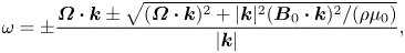 \begin{equation} \omega = {\pm}\frac{\boldsymbol\varOmega\boldsymbol{\cdot}\boldsymbol{k} \pm \sqrt{(\boldsymbol\varOmega\boldsymbol{\cdot}\boldsymbol{k})^2 + |\boldsymbol{k}|^2 (\boldsymbol{B}_0 \boldsymbol{\cdot}\boldsymbol{k})^2/(\rho\mu_0)} } {|\boldsymbol{k}|}, \end{equation}
where  $\omega$ is the frequency, $\boldsymbol{k}$ is the wavenumber vector, $\rho$ is the density and $\mu _0$ is the magnetic permeability. This yields a wide variety of magnetic Coriolis (MC) waves, including fast (modified inertial) and slow (magnetostrophic) waves, the latter being unique to rotating magnetohydrodynamics (MHD). In this paper we consider magnetostrophic waves for which $(\boldsymbol \varOmega \boldsymbol {\cdot }\boldsymbol{k} )^2/|\boldsymbol{k} |^2 \gg (\boldsymbol{B} _0\boldsymbol {\cdot }\boldsymbol{k} )^2/(\rho \mu _0)$: in particular, one class which has the relation
 \begin{equation} \omega \approx - \frac{(\boldsymbol{B}_0 \boldsymbol{\cdot} \boldsymbol{k})^2 |\boldsymbol{k}|^2 }{ \rho\mu_0\beta k } . \end{equation}
Here  $\beta$ denotes the beta parameter, $k$ is the azimuthal wavenumber, and the minus sign indicates that waves travel opposite to the hydrodynamic Rossby wave, $\omega = \beta k/|\boldsymbol{k} |^2$. This class is sometimes referred to as slow hydromagnetic–planetary or magnetic–Rossby (MR) waves (Hide Reference Hide1966). Relation (1.2) indicates that they are dispersive, and depend on the background field and the wavelength; these waves have been suggested to be important in the Earth's fluid core and for the geomagnetic westward drift (e.g. Hide Reference Hide1966; Malkus Reference Malkus1967; Canet, Finlay & Fournier Reference Canet, Finlay and Fournier2014; Hori, Jones & Teed Reference Hori, Jones and Teed2015; Nilsson et al. Reference Nilsson, Suttie, Korte, Holme and Hill2020).
Other classes of MC waves include torsional Alfvén waves, for which  $\boldsymbol \varOmega \boldsymbol {\cdot }\boldsymbol{k} \approx 0$ and $(\boldsymbol \varOmega \boldsymbol {\cdot }\boldsymbol{k} )^2/|\boldsymbol{k} |^2 \ll (\boldsymbol{B} _0\boldsymbol {\cdot }\boldsymbol{k} )^2/(\rho \mu _0)$ (Braginskiy Reference Braginskiy1970; Roberts & Aurnou Reference Roberts and Aurnou2012; Gillet, Jault & Finlay Reference Gillet, Jault and Finlay2015). More recently inertial–Alfvén waves (Bardsley & Davidson Reference Bardsley and Davidson2016) have been suggested to account for the geomagnetic jerks (Aubert & Finlay Reference Aubert and Finlay2019). Laboratory experiments have identified several types of magnetostrophic waves in spherical Couette flows with a dipolar magnetic field being applied (Schmitt et al. Reference Schmitt, Alboussière, Brito, Cardin, Gagnière, Jault and Nataf2008). We note that the wave dynamics relies on both the direction and the morphology of the background magnetic field, as illustrated in the simple planar model (1.2). Here we focus on the problem with a purely azimuthal basic field; for this case (1.2) reduces to $\omega \propto k |\boldsymbol{k} |^2$, indicating its linear and cubic relationship to the azimuthal wavenumber.
The linear theory for MC waves in stably stratified thin layers has been well studied (e.g. Braginskiy Reference Braginskiy1967; Gilman Reference Gilman2000; Zaqarashvili et al. Reference Zaqarashvili, Oliver, Ballester and Shergelashvili2007; Márquez-Artavia, Jones & Tobias Reference Márquez-Artavia, Jones and Tobias2017) as observational exploration of the geomagnetic field and the solar corona has developed to reveal periodic patterns (Chulliat, Alken & Maus Reference Chulliat, Alken and Maus2015; McIntosh et al. Reference McIntosh, Cramer, Marcano and Leamon2017). Stratification in general introduces a correction term to the dispersion relations of MC waves, whilst in a thin layer the direction of travel is usually reversed; however, this is not always true in spherical geometries. The unstratified thick-shell problem considered here is sufficient to provide some fundamental understanding of the nonlinear problem.
Theoretical investigation is expanding to consider their nonlinear properties such as turbulence (Tobias, Diamond & Hughes Reference Tobias, Diamond and Hughes2007) and triadic resonances (Raphaldini & Raupp Reference Raphaldini and Raupp2015). London (Reference London2017) found a couple of cases in which nonlinear equatorial waves in the shallow-water MHD should be governed by Korteweg–de Vries (KdV) equations and so behave like solitary waves. They were mostly fast MR modes, recovering the equatorial Rossby wave soliton (Boyd Reference Boyd1980) in the non-magnetic limit, but he reported one case in which the wave would slowly travel in the opposite azimuthal direction. Hori (Reference Hori2019) investigated magnetostrophic MR waves in a Cartesian quasi-geostrophic (QG) model. The slow, weakly nonlinear waves led to evolution obeying the KdV equation unless the basic state – all the magnetic field, topography and zonal flow – is uniform. Slow MR waves have been seen in spherical dynamo direct numerical simulations (DNS) travelling with crests/troughs that were isolated and sharp, unlike the continuous wave trains that might be expected (Hori et al. Reference Hori, Jones and Teed2015; Hori, Teed & Jones Reference Hori, Teed and Jones2018).
Hydrodynamic Rossby wave solitons have been extensively studied, motivated by atmosphere and ocean dynamics (e.g. Clarke Reference Clarke1971; Redekopp Reference Redekopp1977; Boyd Reference Boyd1980). In the long-wave limit it has been demonstrated that the QG soliton relies on the presence of a shear in the basic flow or topography. Redekopp (Reference Redekopp1977) further analysed nonlinear critical layers arising from singularities as the wave speed approaches the basic flow speed, and discussed their relevance for the persistence of Jupiter's Great Red Spot.
The present paper demonstrates that weakly nonlinear slow MR waves in spherical containers yield soliton solutions. We adopt simple QG MHD models and asymptotically derive the evolution equation for the long waves when the basic magnetic field and flow are both azimuthal. We demonstrate that:
(i) the amplitude at the first order is described by the KdV equation for the chosen basic states;
(ii) the problem is dictated by an ordinary differential equation (ODE), which has no singularities as the wave speed approaches the basic flow speed; and
(iii) the single-soliton (solitary wave) solution to the KdV equation implies an isolated eddy that progresses in a stable permanent form on magnetostrophic time scales.
2. Theoretical foundations
We consider an inviscid, incompressible, ideal QG model of electrically conducting fluid within a rapidly rotating shell, bounded by inner and outer spheres of radii  $r_{i}$ and $r_{o}$, respectively (e.g. Busse Reference Busse1970; Gillet & Jones Reference Gillet and Jones2006). We use polar coordinates $(s,\varphi ,z)$ with rotation $\varOmega \hat {\boldsymbol{z} }$.
For rapid rotation, the incompressible horizontal QG fluid motion can be expressed as  $\boldsymbol{u} \approx \boldsymbol {\nabla } \times \psi (s, \varphi ) \hat {\boldsymbol{z} }$, with $\psi$ a streamfunction, so it is independent of $z$. When the magnetic field is not too strong to violate the QG approximation, we further assume that the magnetic field may be written as $\boldsymbol{B} \approx \boldsymbol {\nabla } \times g (s, \varphi ) \hat {\boldsymbol{z} }$, with $g$ being the potential (e.g. Busse Reference Busse1976; Abdulrahman et al. Reference Abdulrahman, Jones, Proctor and Julien2000; Tobias et al. Reference Tobias, Diamond and Hughes2007; Canet et al. Reference Canet, Finlay and Fournier2014). No penetration on the spherical boundaries at $z=\pm H = \pm \sqrt {r_{o}^2 - s^2}$ enables us to represent the Coriolis term of the axial vorticity equation in terms of the topography-induced beta parameter. The equations for the $z$-components of the vorticity and the magnetic potential in dimensionless form are then
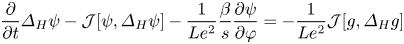 \begin{equation} \frac{\partial}{\partial t} \varDelta_{H} \psi - \mathcal{J} [ \psi, \varDelta_{H} \psi ] - \frac{1}{Le^2} \frac{\beta}{s} \frac{\partial \psi}{\partial \varphi} = - \frac{1}{Le^2} \mathcal{J} [ g, \varDelta_{H} g] \end{equation}
and
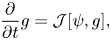 \begin{equation} \frac{\partial}{\partial t} g = \mathcal{J} [ \psi, g ], \end{equation}
where  $\varDelta _{H} = (1/s) \partial /\partial s (s \partial /\partial s) + ( 1/s^2 ) \partial ^2/\partial \varphi ^2$, and $\mathcal {J} [f_1,f_2] = ( (\partial f_1/\partial s)\,(\partial f_2/\partial \varphi)-$ $(\partial f_2/\partial s)\,(\partial f_1/\partial \varphi ) )/s$ for any functions $f_1$ and $f_2$. Here the length, the magnetic field and the velocity are, respectively, scaled by the radius of the outer sphere $r_{o}$, the mean field strength $B_0$ and the MC wave speed $B_0^2/(2\varOmega r_{o} \rho \mu _0) = c_{M}^2/c_{C}$, with $c_{M}^2 = B_0^2/(\rho \mu _0)$ and $c_{C} = 2\varOmega r_{o}$. The Lehnert number $Le = c_{M}/c_{C}$, whilst the beta parameter is given by $\beta = s/(1 - s^2)$. Impermeable boundary conditions are applied so that
 \begin{equation} \frac{1}{s} \frac{\partial \psi}{\partial \varphi}= 0 \quad \textrm{at}\ s = \eta, 1 , \end{equation}
where the aspect ratio  $\eta = r_{i}/r_{o}$. As $\beta \to \infty$ at $s=1$, the governing equations are singular there; these boundary conditions ensure that the regular solution is selected.
Of particular interest is the regime when  $Le^{-1}$ is large. Taking the limit leads to a balance between the vortex stretching and the Lorentz term in the vorticity equation:
 \begin{equation} \beta \frac{1}{s} \frac{\partial \psi}{\partial \varphi} = \mathcal{J} [ g, \varDelta_{H} g] , \end{equation}
whilst (2.2) retains its same form. The nonlinear problems have two source terms acting on the magnetostrophic wave: below, we asymptotically solve the weakly nonlinear cases.
To seek solitary long-wave solutions we introduce slow variables with a small parameter  $\epsilon$ ( $\ll 1)$ and a real constant $c$:
$c$:
 \begin{equation} \tau = \epsilon^{3/2} t, \quad \zeta = \epsilon^{1/2} (\varphi - c t). \end{equation}
Note that this assumes a long spatial scale in the azimuthal direction compared with the radial direction. This is reasonable for small azimuthal wavenumbers. We then expand variables with  $\epsilon$ as
 \begin{equation} \psi = \psi_0 (s) + \epsilon \psi_1 (s,\zeta,\tau) + \cdots, \quad g = g_0 (s) + \epsilon g_1 (s,\zeta,\tau) + \cdots, \end{equation}
for the basic state satisfying
 \begin{equation} {-}\textrm{D} \psi_0 = \bar{U}(s), \quad {-}\textrm{D} g_0 = \bar{B}(s), \end{equation}
where  $\textrm {D} = \textrm {d}/\textrm {d}s$. At zeroth order the equations of vorticity (2.4) and of electric potential (2.2) and the boundary condition (2.3) are all trivial.
At  $ {O}(\epsilon )$, (2.4) and (2.2) become
 \begin{equation} \beta \frac{\partial \psi_1}{\partial \zeta} = - \left[ \bar{B} \mathcal{D}^2 - \bar{J} \right] \frac{\partial g_1}{\partial \zeta}, \quad \text{where} \quad \mathcal{D}^2 = \frac{1}{s} \frac{\partial}{\partial s} s \frac{\partial}{\partial s} \quad \text{and} \quad \bar{J} = \textrm{D} \frac{1}{s} \, \textrm{D} (s \bar{B}), \end{equation}
and
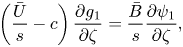 \begin{equation} \left( \frac{\bar{U}}{s} - c \right) \frac{\partial g_1}{\partial \zeta} = \frac{\bar{B}}{s} \frac{\partial \psi_1}{\partial \zeta}, \end{equation}
respectively. Substituting (2.8) into (2.9) gives a homogeneous partial differential equation (PDE) with respect to  $g_1$:
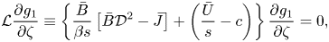 \begin{equation} \mathcal{L} \frac{\partial g_1}{\partial \zeta} \equiv \left\{ \frac{\bar{B}}{ \beta s} \left[ \bar{B} \mathcal{D}^2 - \bar{J} \right] + \left( \frac{\bar{U} }{s} - c \right) \right\} \frac{\partial g_1}{\partial \zeta} = 0, \end{equation}
where  $\mathcal {L}$ represents the linear differential operator comprising $s,\,$ $\bar {B},\beta , \bar {U}$ and $c$. Inserting the boundary conditions (2.3) at this order into (2.9) yields
 \begin{equation} \frac{\partial g_1}{\partial \zeta} = 0 \quad \text{at}\ s = \eta , 1. \end{equation}
We then seek a solution in the form of  $g_1 = \varPhi (s) G(\zeta ,\tau )$, so that
 \begin{equation} \mathcal{L} \varPhi = 0 \quad \mbox{and } \quad \varPhi = 0 \quad\text{at}\ s = \eta, 1 . \end{equation}
Now the linear operator  $\mathcal {L}$ is the ordinary differential operator with the partial derivatives with respect to $s$ replaced by D. Given a basic state, the ODE (2.12) together with the boundary conditions is an eigenvalue problem to determine the eigenfunction $\varPhi$ with eigenvalue $c$; it can have many eigensolutions. We note that the second-order ODE (2.12a) remains non-singular as $\bar {U}/s \rightarrow c$, but not as $\bar {B}^2/\beta \rightarrow 0$ unless $s = 0$. Below, we concentrate on cases in which (2.12a) has no internal singularities, i.e. there is a discrete spectrum. We consider cases where the $z$-averaged toroidal magnetic fields do not pass through zero (e.g. figure 3 of Schaeffer et al. (Reference Schaeffer, Jault, Nataf and Fournier2017); figures 1 and 2 of Hori et al. (Reference Hori, Teed and Jones2018)).
We proceed to the next order to obtain the amplitude function. Equations (2.4) and (2.2) at  $ {O}(\epsilon ^2)$ yield
 \begin{equation} \beta \frac{\partial \psi_2}{\partial \zeta} = - \left[ \bar{B} \mathcal{D}^2 - \bar{J} \right] \frac{\partial g_2}{\partial \zeta} - \frac{\bar{B}}{s^2} \frac{\partial^3 g_1}{\partial \zeta^3} + \left( \frac{\partial g_1}{\partial s} \frac{\partial}{\partial \zeta} - \frac{\partial g_1}{\partial \zeta} \frac{\partial}{\partial s} \right) \mathcal{D}^2 g_1 \end{equation}
and
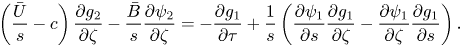 \begin{equation} \left( \frac{\bar{U}}{s} - c \right) \frac{\partial g_2}{\partial \zeta} - \frac{\bar{B}}{s} \frac{\partial \psi_2}{\partial \zeta} = - \frac{\partial g_1}{\partial \tau} + \frac{1}{s} \left( \frac{\partial \psi_1}{\partial s} \frac{\partial g_1}{\partial \zeta} - \frac{\partial \psi_1}{\partial \zeta}\frac{\partial g_1}{\partial s} \right) . \end{equation}
Eliminating  $\psi _2$ using (2.13) and $\psi _1$ using (2.8), (2.14) becomes the inhomogeneous PDE
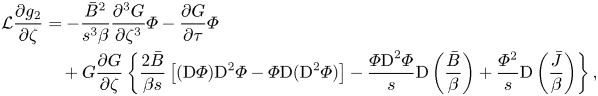 \begin{align} \mathcal{L} \frac{\partial g_2}{\partial \zeta} & = - \frac{\bar{B}^2}{s^3 \beta} \frac{\partial^3 G}{\partial \zeta^3} \varPhi - \frac{\partial G}{\partial \tau} \varPhi \nonumber\\ &\quad + G \frac{\partial G}{\partial \zeta} \left\{ \frac{2\bar{B}}{\beta s} \left[ (\textrm{D} \varPhi) \textrm{D}^2 \varPhi - \varPhi \textrm{D} (\textrm{D}^2 \varPhi) \right] - \frac{\varPhi \textrm{D}^2 \varPhi}{s} \textrm{D} \left(\frac{\bar{B}}{\beta} \right) + \frac{\varPhi^2}{s} \textrm{D} \left(\frac{\bar{J}}{\beta} \right) \right\}, \end{align}
where  $\textrm {D}^2 = (1/s) \textrm {D} s \textrm {D}$. The boundary conditions here are
 \begin{equation} \frac{\partial g_2}{\partial \zeta} = 0 \quad \textrm{at}\ s = \eta , 1. \end{equation}
The adjoint linear problem corresponding to (2.10) is
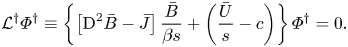 \begin{equation} \mathcal{L}^{\dagger} \varPhi^{\dagger} \equiv \left\{ \left[ \textrm{D}^2 \bar{B} - \bar{J} \right] \frac{\bar{B}}{\beta s } + \left( \frac{\bar{U}}{s} - c \right) \right\} \varPhi^{\dagger} = 0 . \end{equation}
The adjoint boundary conditions are
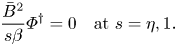 \begin{equation} \frac{\bar{B}^2}{s\beta} \varPhi^{\dagger} = 0 \quad \textrm{at}\ s = \eta , 1. \end{equation}
Note that the substitution  $\bar {B}^2 \varPhi ^{\dagger} / s \beta = \varPhi$ reduces the adjoint problem to the ordinary linear problem (2.12) so, provided $\bar {B}^2 \varPhi ^{\dagger} /s\beta$ is non-zero in the sphere, the adjoint eigenfunction $\varPhi ^{\dagger}$ can simply be found by dividing the solution of (2.12) by $\bar {B}^2/s\beta$.
The solvability condition to (2.15) is thus given by
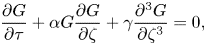 \begin{equation} \frac{\partial G}{\partial \tau} + \alpha G \frac{\partial G}{\partial \zeta} + \gamma \frac{\partial^3 G}{\partial \zeta^3} = 0, \end{equation}
where  $\alpha = \alpha _0/\delta _0$, $\gamma = \gamma _0/\delta _0$,
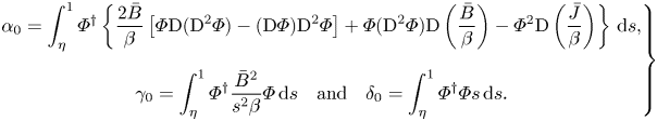 \begin{equation} \left. \begin{gathered} \alpha_0 = \int _{\eta}^1 \varPhi^{\dagger} \left\{ \frac{2\bar{B}}{\beta} \left[ \varPhi \textrm{D} (\textrm{D}^2 \varPhi) - (\textrm{D} \varPhi) \textrm{D}^2 \varPhi \right] + \varPhi (\textrm{D}^2 \varPhi) \textrm{D}\left(\frac{\bar{B}}{\beta} \right) - \varPhi^2 \textrm{D}\left(\frac{\bar{J}}{\beta} \right) \right\} \,\textrm{d}s, \\ \gamma_0 = \int_{\eta}^{1} \varPhi^{\dagger} \frac{\bar{B}^2}{s^2 \beta} \varPhi \,\textrm{d}s \quad \textrm{and} \quad \delta_0 = \int_{\eta}^{1} {\varPhi^{\dagger} \varPhi} s \, \textrm{d}s . \end{gathered} \right\} \end{equation}
Equation (2.19) is the KdV equation if the coefficients,  $\alpha$ and $\gamma$, are both non-zero. In the following section we examine the coefficients for different choices of the basic state.
We note that the presence of  $\bar {U}$ does not directly impact either $\alpha$ or $\gamma$. It, however, dictates $\varPhi$ and $\varPhi ^{\dagger}$ through the linear problems at $ {O}(\epsilon )$ and then may contribute to the terms at $ {O}(\epsilon ^2)$. This is in contrast with the hydrodynamic case (e.g. Redekopp Reference Redekopp1977), where the basic flow enters the nonlinear term at $ {O}(\epsilon ^2)$ too. The mean-flow effect on the magnetostrophic wave arises from the equation for the magnetic potential (2.2).
Solutions to (2.19) may take the form of solitary (single or multiple soliton), cnoidal, similarity and rational waves (e.g. Whitham Reference Whitham1974; Drazin & Johnson Reference Drazin and Johnson1989). For instance, for a single soliton the asymptotic solution up to  $ {O}(\epsilon )$ is
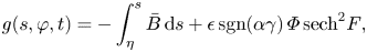 \begin{gather} g (s,\varphi, t) = -\int_{\eta}^{s} \bar{B}\,\textrm{d}s + \epsilon \, \mathrm{sgn}(\alpha \gamma) \, \varPhi \,{\mathrm{sech}^2 F}, \end{gather}
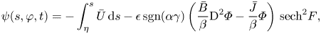 \begin{gather}\psi (s,\varphi, t) = -\int_{\eta}^{s} \bar{U}\,\textrm{d}s - \epsilon \, \mathrm{sgn}(\alpha \gamma) \left( \frac{\bar{B}}{\beta} \textrm{D}^2 \varPhi - \frac{\bar{J}}{\beta} \varPhi \right) \, {\mathrm{sech}^2 F}, \end{gather}
where
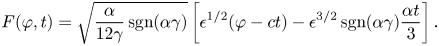 \begin{equation} F (\varphi, t) = \sqrt{ \frac{\alpha }{12 \gamma} \,\mathrm{sgn}(\alpha \gamma) } \left[ \epsilon^{1/2} (\varphi -ct) - \epsilon^{3/2} \, \mathrm{sgn}(\alpha \gamma) \frac{\alpha t}{3} \right]. \end{equation}
This is an eddy that has the solitary characteristics in azimuth, riding on the basic state with the linear wave speed. The finite-amplitude effect  $\alpha$ accelerates the retrograde propagation if $\gamma < 0$, but decelerates it when $\gamma > 0$. The characteristic waveform is clearly visible in the magnetic potential.
3. Illustrative examples
We solve the eigenvalue problem (2.12) and the adjoint problem (2.17)–(2.18) for different basic states and calculate the respective coefficients of the evolution equation (2.19) in a spherical cavity with  $\eta = 0.35$. We consider the three cases investigated in Canet et al. (Reference Canet, Finlay and Fournier2014): the first has a $\bar {B}$ that is a linearly increasing function of $s$ (referred to as a Malkus field hereafter); the second $\bar {B}$ is inversely proportional to $s$ (an electrical wire field); and the third one is $(3/2) \cos \{ {\rm \pi}(3/2 - 50 s/19) \} + 2$, which was adopted by Canet et al. (Reference Canet, Finlay and Fournier2014) to model a profile of the radial magnetic field $B_s$ within the Earth's core (which we term a Canet–Finlay–Fournier (CFF) field). For the Malkus and wire fields, the terms $\bar {J}$ in (2.12), (2.17) and (2.20) all vanish, whereas this is not the case for the CFF field. The Malkus field case has been extensively studied in the literature (e.g. Malkus Reference Malkus1967; Roberts & Loper Reference Roberts and Loper1979; Zhang, Liao & Schubert Reference Zhang, Liao and Schubert2003; Márquez-Artavia et al. Reference Márquez-Artavia, Jones and Tobias2017). We also consider the inclusion of a basic zonal flow $\bar {U}$ that is prograde, with either a linear or quadratic dependence on $s$.
$s$.
Table 1 summarises the results, listing the eigenvalue  $\lambda = \sqrt {|c|}/2$ (see below) and $c$ for the $n$th mode, the coefficients $\alpha$, $\gamma$ and $\delta _0$ as calculated from the eigenfunction $\varPhi$, the adjoint eigensolution $\varPhi ^{\dagger}$ and (2.20), and whether/at which $s$ the wave speed $c$ approaches the basic angular velocity $\bar {U}/s$. Here the $n$th mode has $(n-1)$ zeros within the explored interval. Negative values of $c$ indicate retrograde waves. More notably, in all the cases we obtain non-zero $\alpha$ and $\gamma$ for all $n$ examined and so the KdV equations are appropriate. The fraction $|\alpha /\gamma |$ and their signs characterise the solitons.
Table 1. Values of  $\lambda$, $c$,
$c$,  $\alpha$, $\gamma$ and $\delta _0$ of the $n$th mode for the basic magnetic field $\bar {B}$ and flow $\bar {U}$ in the spherical model $\beta = s/(1-s^2)$. The CFF field $\bar {B}$ is given as $(3/2) \cos \{ {\rm \pi}(3/2 - 50 s/19) \} + 2$. Cases indicated by $^\circ$ are evaluated with the routine bvp4c and the modified outer boundary condition.

For the Malkus field ( $\bar {B} = s$) and no mean flow $\bar {U}$, we let $x = 1-s^2$ and $\varPhi (x) = x y(x)$ to rewrite the ODE (2.12) as
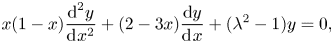 \begin{equation} x(1-x) \frac{\textrm{d}^2 y}{\textrm{d}\kern0.7pt x^2} + (2-3x) \frac{\textrm{d}y}{\textrm{d}\kern0.7pt x} + (\lambda^2 -1) y =0, \end{equation}
where  $\lambda ^2 = - c/4$. This is a hypergeometric equation, which has a solution
 \begin{equation} \varPhi (s) = (1-s^2)\, F(1+\lambda, 1-\lambda; 2; 1-s^2),\quad \textrm{and} \quad \varPhi^{\dagger} = \frac{\varPhi}{1-s^2} , \end{equation}
where  $F$ denotes the hypergeometric function (e.g. Abramowitz & Stegun Reference Abramowitz and Stegun1965). The eigenvalue $\lambda$ is determined by the condition $\varPhi =0$ at $s=\eta$. The adjoint solution is related to the axial electrical current generated at this order as $-\textrm {D}^2 \varPhi = -c \varPhi s\beta /\bar {B}^2 = -c \varPhi ^{\dagger}$, implying that the current is non-zero at $s=1$.
Figure 1 shows the solutions in the Malkus case. Figure 1(a) shows profiles of  $\bar {B}(s)$, the topography $\beta$, the eigenfunctions $\varPhi$ for $n = 1$ and $2$, and their adjoint eigenfunctions $\varPhi ^{\dagger}$ (3.2a,b). This yields $\alpha \approx -12.85$ and $\gamma \approx 0.87$ for $n=1$; the nonlinear effect is more significant than the dispersive one. Figure 1(b) illustrates a single-soliton solution (2.22) of $\psi$ for $n=1$. If the amplitude $\epsilon$ is too large, neglected higher-order terms will be significant; if $\epsilon$ is too small, the azimuthal scale of the solitary wave is too large to fit in, so we choose $\epsilon = 0.1$ as a reasonable compromise. The streamfunction $\psi$ is negative, indicating a clockwise solitary eddy. The retrogradely propagating vortex $\psi _1$ is slightly more concentrated at the outer shell than the magnetic potential $g_1$ (not shown). As $c < 0$ and $\gamma > 0$, the dispersion term reduces the retrograde propagation speed. We note that a clockwise vortex is observed in the Earth's core (Pais & Jault Reference Pais and Jault2008) and geodynamo simulations (Schaeffer et al. Reference Schaeffer, Jault, Nataf and Fournier2017): its implications are discussed in the final section.
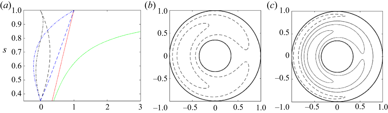
Figure 1. Spherical case for the Malkus field  $\bar {B}=s$ and $\bar {U}=0$. $(a)$ Profiles of $\bar {B}$ (red solid curve), $\beta$ (green solid), $\varPhi$ for $n=1$ (black dashed) and $n=2$ (black dashed-dotted), and $\varPhi ^{\dagger}$ for $n=1$ (blue dashed) and $n=2$ (blue dashed-dotted). (b,c) Streamfunctions $\psi$ of the single-soliton solution for $(b)$
$(b)$ $n=1$ and $(c)$
$(c)$ $n=2$, provided $\epsilon = 0.1$. The dashed (solid) contour lines represent its negative (positive) value, i.e. clockwise (anticlockwise).
The same basic states admit high- $n$ modes with more isolated structure to have the KdV equations with non-zero $\alpha$ and $\gamma$ (table 1). The speed $|c|$ increases with $n$, confirming the dispersivity of the wave. The eigenfunction $\varPhi$ for $n=2$ is negative at small $s$, and then turns positive when $s \gtrsim 0.787$ (dashed-dotted curve in Figure 1a), so the eddy is clockwise in the outer region and anticlockwise in the inner region (Figure 1c).
We next consider the basic field given by the wire field,  $\bar {B} = 1/s$, whilst $\bar {U} = 0$. By using $\varPhi (x) = x \,\textrm {e}^{\lambda x} y(x)$, (2.12) may be reduced to a confluent Heun equation
 \begin{align} x(1-x) \frac{\textrm{d}^2 y}{\textrm{d}\kern0.7pt x^2} + \{2 + (2 \lambda -3)x -2 \lambda x^2 \} \frac{\textrm{d}y}{\textrm{d}\kern0.7pt x} + \{ (\lambda^2 +2 \lambda -1) - (\lambda^2+3 \lambda)x\}y =0 . \end{align}
The solution regular at  $s=1$ corresponding to the eigenvalue $\lambda$ is
 \begin{equation} \varPhi = (1-s^2) \textrm{e}^{\lambda(1-s^2)} H_{c}(q_{c}, \alpha_{c}, \gamma_{c},\delta_{c},\epsilon_{c}; 1-s^2),\quad \textrm{and} \quad \varPhi^{\dagger} = \frac{s^4}{1-s^2} \varPhi , \end{equation}
where  $H_{c}$ represents the confluent Heun function with the accessory parameter $q_{c} =\lambda ^2 +2 \lambda - 1$ and exponent parameters $\alpha _{c} = \lambda ^2 + 3 \lambda ,\ \gamma _{c} = 2,\ \delta _{c} = 1$ and $\epsilon _{c} = 2 \lambda$ (Olver et al. Reference Olver, Lozier, Boisvert and Clark2010). This case admits a simple form of the coefficients (2.20) such that
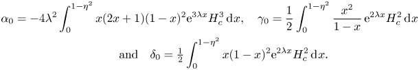 \begin{gather} \alpha_0 = -4 \lambda^2 \int^{1-\eta^2}_0 x (2x+1) (1-x)^2 \textrm{e}^{3\lambda x} H_{c}^3 \,\textrm{d}\kern0.7pt x , \quad \gamma_0 = \frac{1}{2} \int^{1-\eta^2}_{0} \frac{x^2}{1-x}\, \textrm{e}^{2\lambda x} H_{c}^2 \, \textrm{d}\kern0.7pt x \nonumber\\ \qquad\quad \text{and} \quad \delta_0 = \tfrac{1}{2} \int^{1-\eta^2}_{0} x(1-x)^2 \textrm{e}^{2\lambda x} H_{c}^2 \,\textrm{d}\kern0.7pt x . \end{gather}
To evaluate the function we use the algorithm of Motygin (Reference Motygin2018) below.
Figure 2(a) gives profiles of the basic state and eigenfunctions. The figure shows that  $\varPhi$ for $n=1$ has a peak nearer the outer boundary, compared with that for the Malkus field; it is still propagating retrogradely and is dispersive. This case yields $\alpha \approx -36.9$ and $\gamma \approx 1.25$ for $n=1$ and with $\epsilon =0.1$ the soliton is a more compact, clockwise eddy (Figure 2b). Analysis of the individual terms of the coefficient $\alpha _0$ in (2.20a) implies that the presence of high-order derivatives is favourable for nonlinear effects. For $n=2$, dispersive effects are enhanced compared to nonlinear ones. The solitary eddy is clockwise in the outer region when $s \gtrsim 0.894$ and anticlockwise in the inner region (Figure 2c).

Figure 2. Spherical case for the wire field  $\bar {B}=1/s$ and $\bar {U}=0$. $(a)$ Profiles of $\bar {B}$ (red solid curve), $\beta$ (green solid), $\varPhi$ for $n=1$ (black dashed) and $n=2$ (black dashed-dotted), and $\varPhi ^{\dagger}$ for $n=1$ (blue dashed) and $n=2$ (blue dashed-dotted). (b,c) Streamfunctions $\psi$ of the single-soliton solution for $(b)$
$(b)$ $n=1$ and $(c)$
$(c)$ $n=2$, provided $\epsilon = 0.1$.
To explore more general cases, we implement the MATLAB routine bvp4c to solve the eigenvalue problems. We retain the boundary condition  $\varPhi = 0$ at $s = \eta = 0.35$, but use the modified condition $\varPhi + (1-s) {\textrm {D}\varPhi } = 0$ close to the outer boundary $s=0.99999$ to avoid the numerical issue arising from singularities when $s \rightarrow 1$. We also impose a normalising condition $\textrm {D}\varPhi$ at the inner boundary: the values for the Malkus field and the CFF field are given by (3.2a), whereas the one for the wire field is given by (3.4a). The number of grid points in $s$ is $500$ in all cases. Given the obtained $c$, the same routine is adopted to solve the boundary value problems for $\varPhi ^{\dagger}$. For consistency with the earlier cases we set $\varPhi ^{\dagger} = 1$ at the outer boundary. The codes are benchmarked with the exact solutions. With modified boundary condition, our computational results match the expected eigenvalues $\lambda = \sqrt {|c|}/2$ and eigenfunctions $\varPhi$ for $1 \le n \le 3$ with errors less than 0.01 % and 0.2 %, respectively.
Now the third basic field,  $\bar {B} = (3/2) \cos \{ {\rm \pi}(3/2 - 50 s/19) \} + 2$, is examined. Figure 3(a) depicts the basic state, the eigenfunctions for $n=1$ and additionally $\bar {J}$ (represented by the red dotted curve). It is non-zero except at $s \approx 0.40$ and $0.78$ and is negatively peaked at $s \approx 0.59$. The eigenvalues $c$ do not differ from those in the Malkus case very much (table 1). For $n=1$, $\varPhi$ has a peak at $s \approx 0.61$ (blue dashed curve), and so does the basic field. This case gives $\alpha \approx -11.5$ and $\gamma \approx 2.85$. Indeed, the term including $\bar {J}$ dominates over the ODE (2.12a) and also over $\alpha _0$ (2.20a); if the term $\varPhi ^2 \textrm {D}(\bar {J}/\beta )$ were absent, $\alpha$ would become $\approx 1.68$. Figure 3(b) illustrates the magnetic potential $g_1$ (2.21), where the basic state is excluded for visualisation. It is clockwise and centred at $s \approx 0.61$. Similarly, the streamfunction $\psi$ (2.22) is displayed in Figure 3(c): now the distinction from the magnetic component is evident. The solitary eddy is more confined nearer the outer boundary, as $\bar {B} \textrm {D}^2 \varPhi - \bar {J}\varPhi$ in (2.22) becomes significant only when $s \gtrsim 0.8$ (not shown).

Figure 3. Spherical case for the CFF field  $\bar {B}=(3/2) \cos \{ {\rm \pi}(3/2 - 50s/19) \} + 2$, $\bar {U}=0$ and $n=1$. $(a)$ Profiles of $\bar {B}$ (red solid curve), $\beta$ (green solid), $\bar {J}$ (red dotted; normalised for visualisation), $\varPhi$ (black dashed), and $\varPhi ^{\dagger}$ (blue dashed). (b) Magnetic potential $g_1$ of the single-soliton solution, where the basic state $g_0$ is excluded to help visualisation. $(c)$ Streamfunctions $\psi$ of the solution, provided $\epsilon = 0.1$.
Including a basic flow  $\bar {U} = s$ is equivalent to the addition of solid-body rotation. Therefore, it affects the speed $c$ of propagation of the mode, whilst leaving its other properties unchanged (table 1). For a more realistic flow, $\bar {U} = 4 s(1-s)$, with the Malkus field, the structures of $\varPhi$ and $\varPhi ^{\dagger}$ are not drastically altered (leading to $\delta _0 \approx 0.049$). The dominance of the nonlinearity over the dispersion, $|\alpha /\gamma |$, is, however, weakened. The presence of the same basic flow in the wire field case also exhibits this property.
Finally, we comment on the behaviour of solutions in the vicinity of the point  $s$ at which $\bar {U}/s$ equals $c$, the location of a critical layer for the hydrodynamic Rossby wave soliton (e.g. Redekopp Reference Redekopp1977). We impose a fast mean zonal flow, $\bar {U} = 80 s(1-s)$, in the Malkus field case; Figure 4(a) shows the basic state and additionally the deviation from the wave speed, $\bar {U}/s - c$ (blue dotted curve). The curve shows that this case has such a critical point at $s \approx 0.838$. Nevertheless, the impact is hardly seen in the eigenfunctions $\varPhi$ and $\varPhi ^{\dagger}$: there are no discontinuities in the derivative $\textrm {D}\varPhi$ (Figure 4b) and hence in the solitary wave solutions (Figure 4c). This remains true for the wire field and the CFF field with $\bar {U}=320s(1-s)$.
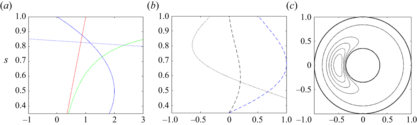
Figure 4. Spherical case for the Malkus field  $\bar {B}=s$, the basic flow $\bar {U} = 80s(1-s)$ and $n=1$. $(a)$ Profiles of $\bar {B}$ (red solid curve), $\beta$ (green solid), $\bar {U}/10$ (blue solid; scaled for visualisation), and the deviation $\bar {U}/s - c$ (blue dotted). $(b)$ Profiles of $\varPhi$ (black dashed), $\varPhi ^{\dagger}$ (blue dashed), and $\textrm {D} \varPhi$ (black dotted). $(c)$ Streamfunction $\psi _1$ of the single-soliton solution, where the basic state $\psi _0$ is excluded to help visualisation.
4. Concluding remarks
In this paper we have performed a weakly nonlinear analysis of magnetostrophic waves in QG spherical models with azimuthal magnetic fields and flows. The model we considered is an annulus model (Busse Reference Busse1976; Canet et al. Reference Canet, Finlay and Fournier2014) of the form utilised by Hide (Reference Hide1966) for linear magnetic Rossby (MR) waves. We found that the evolution of the long-wavelength, slow-MR waves in the spherical shells obeyed the KdV equation, whether the toroidal magnetic field and/or the zonal flow were sheared or not. The model we consider here is formally valid for cases where the azimuthal length scale is much longer than that in radius; the most obvious application of which is for thin spherical shells. For thicker spherical shells like those representative of the Earth's fluid outer core, the ratio of these length scales is of the order of 10. For thinner shells relevant to other astrophysical objects, one might expect the asymptotic procedure to give a better approximation to the true behaviour. We find that solutions may take the form of a single-soliton solution (for  $n=1$) which is a clockwise, solitary eddy when the basic state magnetic field is any of a Malkus field ( $\bar {B} \propto s$), a magnetic wire field ( $\bar {B} \propto 1/s$) and a CFF field (comprising a trigonometric function). In addition to these steadily progressing single solitons, we also find $N$-soliton solutions; as these satisfy the KdV equation, we know that these may have peculiar interactions, including a phase shift after a collision and Fermi–Pasta–Ulam recurrence (e.g. Drazin & Johnson Reference Drazin and Johnson1989).
We conclude by noting that inversion of the geomagnetic secular variation appears to detect an anticyclonic gyre in the Earth's core (Pais & Jault Reference Pais and Jault2008; Gillet et al. Reference Gillet, Jault and Finlay2015; Barrois et al. Reference Barrois, Hammer, Finlay, Martin and Gillet2018); it is off-centred with respect to the rotation axis and is believed to have existed for more than a hundred years. Moreover, DNS of dynamos driven by convection in rapidly rotating spherical shells have exhibited the emergence of a large vortex which circulated clockwise and modulated very slowly (Schaeffer et al. Reference Schaeffer, Jault, Nataf and Fournier2017); in these simulations the averaged toroidal magnetic field tended to strengthen beneath the outer boundary. Our solution tentatively supports the idea that such an isolated single eddy should persist, while drifting on MC time scales of  $ {O}(10^{2\text {--}4})$ years. The long wave can be initiated through instabilities due to differentially rotating flows (Schmitt et al. Reference Schmitt, Alboussière, Brito, Cardin, Gagnière, Jault and Nataf2008), due to thermally insulating boundaries (Hori, Takehiro & Shimizu Reference Hori, Takehiro and Shimizu2014), and due to the magnetic diffusivity (Roberts & Loper Reference Roberts and Loper1979; Zhang et al. Reference Zhang, Liao and Schubert2003). The steadily drifting feature of the solitons should, of course, be altered during the long-term evolution when dissipation plays a role in the dynamics. The presence of dissipation may also alter the eigenfunction (Canet et al. Reference Canet, Finlay and Fournier2014) and thus the detailed morphology of the soliton too.
We note that an alternative to account for the eccentric gyre is a flow induced by, for example, the coupling with the rocky mantle and the solid inner core, as DNS by Aubert, Finlay & Fournier (Reference Aubert, Finlay and Fournier2013) had demonstrated. The issue ends up in a debate which has lasted for decades: Does the geomagnetic westward drift represent the advection due to a large-scale fluid motion (Bullard et al. Reference Bullard, Freedman, Gellman and Nixon1950) or hydromagnetic wave motion (Hide Reference Hide1966)? We shall investigate these issues further, as well as the role of critical layers, by solving initial value problems in a future study.
Acknowledgements
The authors are grateful to A. Soward, A. Kalogirou, A. Barker and Y.-Y. Hayashi for discussion and comments. Comments by three anonymous reviewers helped to improve the manuscript. K.H. was supported by the Japan Science and Technology/Kobe University under the programme ‘Initiative for the Implementation of the Diversity Research Environment (Advanced Type)’. C.A.J. acknowledges support from the UK's Science and Technology Facilities Council, STFC research grant ST/S00047X/1.
Declaration of interests
The authors report no conflict of interest.


 Open access