


1. Introduction
The growth of perturbations at an interface between two fluids of different property, driven by an external force or an acceleration field, is generally referred to as the Rayleigh–Taylor (RT) instability (Rayleigh Reference Rayleigh1883; Taylor Reference Taylor1950). A similar hydrodynamic instability is the Richtmyer–Meshkov (RM) instability (Richtmyer Reference Richtmyer1960; Meshkov Reference Meshkov1969), which occurs when a perturbed interface is subjected to an impulsive force typically by a shock wave. Although RM and RT instabilities share common evolution processes such as the formation of bubbles (a light fluid rises into a heavy one) and spikes (a heavy fluid falls freely into a light one), their perturbation growth rates are distinctly different. Specifically, RT perturbation grows exponentially with time at the early stage and later at a constant asymptotic growth rate, whereas RM perturbation grows linearly at the early stage and later nonlinearly at a time-decaying growth rate. Over the past decades, RM instability has attracted widespread attention due to its significance in academic research, e.g. compressible turbulence (Mohaghar et al. Reference Mohaghar, Carter, Pathikonda and Ranjan2019; Groom & Thornber Reference Groom and Thornber2021) and vortex dynamics (Peng et al. Reference Peng, Yang, Wu and Xiao2021), as well as the important role in industrial fields such as inertial confinement fusion (ICF) (Betti & Hurricane Reference Betti and Hurricane2016).
In terms of the flow cross-section area, RM instability can be categorized into two types: area-invariant RM instability and area-varied RM instability. The former usually refers to planar shock-induced RM instability, which has been extensively studied by experimentalists (Biamino et al. Reference Biamino, Jourdan, Mariani, Houas, Vandenboomgaerde and Souffland2015; Reese et al. Reference Reese, Ames, Noble, Oakley and Bonazza2018; Liang et al. Reference Liang, Liu, Zhai, Ding, Si and Luo2021; Sewell et al. Reference Sewell, Ferguson, Krivets and Jacobs2021), theorists (Richtmyer Reference Richtmyer1960; Zhang & Sohn Reference Zhang and Sohn1997; Dimonte & Ramaprabhu Reference Dimonte and Ramaprabhu2010; Zhang & Guo Reference Zhang and Guo2016) and numerical experts (Schilling & Latini Reference Schilling and Latini2010; Lombardini, Pullin & Meiron Reference Lombardini, Pullin and Meiron2014; Wonga & Lelea Reference Wonga and Lelea2017; Li et al. Reference Li, Fu, Yu and Li2022). It is widely accepted that pressure disturbance (caused by pressure waves behind the refracted shock) and baroclinic vorticity (caused by the misalignment of pressure and density gradients) are the major mechanisms for the growth of area-invariant RM instability (Brouillette Reference Brouillette2002; Ranjan, Oakley & Bonazza Reference Ranjan, Oakley and Bonazza2011; Zhou Reference Zhou2017). Two typical representatives of area-varied RM instability are convergent shock-induced RM instability (i.e. convergent RM instability) (Vandenboomgaerde et al. Reference Vandenboomgaerde, Rouzier, Souffland, Biamino, Jourdan, Houas and Mariani2018) and divergent shock-induced RM instability (i.e. divergent RM instability) (Li et al. Reference Li, Ding, Zhai, Si, Liu, Huang and Luo2020). In addition to the flow mechanisms of area-invariant RM instability, the area-varied counterpart involves new physical regimes such as geometric contraction/expansion (Penney & Price Reference Penney and Price1945; Bell Reference Bell1951; Plesset Reference Plesset1954; Epstein Reference Epstein2004) and RT stability/instability caused by flow deceleration (Ding et al. Reference Ding, Si, Yang, Lu, Zhai and Luo2017b; Luo et al. Reference Luo, Zhang, Ding, Si, Yang, Zhai and Wen2018), and thus presents more possibilities and complexities for the instability growth.
Convergent RM instability, which involves an initial setting more relevant to hydrodynamic instabilities in ICF, has become increasingly more attractive in recent years. The first experiments on convergent RM instability were carried out by Hosseini, Ogawa & Takayama (Reference Hosseini, Ogawa and Takayama2000) in a vertical coaxial shock tube. This coaxial shock tube was later improved by Si et al. (Reference Si, Long, Zhai and Luo2015) and Lei et al. (Reference Lei, Ding, Si, Zhai and Luo2017), in which the development of convergent RM instability at a polygonal/single-mode interface was obtained with a high-speed imaging technique. Also, Dimotakis & Samtaney (Reference Dimotakis and Samtaney2006) proposed a gas-lens technique, with which cylindrically/spherically convergent shocks can be generated through shock refraction (Biamino et al. Reference Biamino, Jourdan, Mariani, Houas, Vandenboomgaerde and Souffland2015; Vandenboomgaerde et al. Reference Vandenboomgaerde, Rouzier, Souffland, Biamino, Jourdan, Houas and Mariani2018). Based on shock dynamics theory, a horizontal shock tube with a special wall profile that smoothly transforms an initial planar shock into a cylindrical one was designed by Zhai et al. (Reference Zhai, Liu, Qin, Yang and Luo2010). Recently, clear observation of convergent RM instability was achieved (Ding et al. Reference Ding, Si, Yang, Lu, Zhai and Luo2017b, Reference Ding, Li, Sun, Zhai and Luo2019; Li et al. Reference Li, Ding, Zhai, Si, Liu, Huang and Luo2020) in a novel semi-annular shock tube, and the influences of geometric contraction/expansion and RT instability/stability on the perturbation growth were quantified.
The development of convergent RM instability usually involves two stages: a convergent stage (i.e. instability growth after an incident convergent shock strikes the interface) and a divergent stage (i.e. instability growth after a divergent shock that is reflected from the geometric centre impacts the deforming interface). Previous studies on convergent RM instability were mainly focused on the convergent stage (Ding et al. Reference Ding, Si, Chen, Zhai, Lu and Luo2017a; Vandenboomgaerde et al. Reference Vandenboomgaerde, Rouzier, Souffland, Biamino, Jourdan, Houas and Mariani2018; Ding et al. Reference Ding, Li, Sun, Zhai and Luo2019) and little attention was paid to the divergent stage. The main reasons are given below. First, the interface has been severely distorted before the arrival of the divergent shock. Thus, it is very difficult to accurately characterize the interface shape. Second, the pre-reshock flow field exhibits strong non-uniformity along both radial and circumferential directions, which greatly impedes the flow analysis. It is therefore highly desirable to conduct an experimental study on divergent RM instability with controllable initial conditions, which is essential for understanding the flow regimes at the divergent stage of convergent RM instability. In addition, divergent RM instability is a good approximation of hydrodynamic instability in supernova explosion (Arnett et al. Reference Arnett, Bahcall, Kirshner and Woosley1989; Kuranz et al. Reference Kuranz2018), where stellar collapse produces a spherically divergent shock that passes across multi-layer elements, and thus the relevant study is helpful for explaining the formation of supernova remnant (Miles et al. Reference Miles, Edwards, Blue, Hansen, Robey, Drake, Kuranz and Leibrandt2004; Ribeyre, Tikhonchuk & Bouquet Reference Ribeyre, Tikhonchuk and Bouquet2004; Musci et al. Reference Musci, Petter, Pathikonda, Ochs and Ranjan2020). Moreover, as another typical representative of area-varied RM instability, study on divergent RM instability would complete the fundamental understanding of area-varied RM instability.
A key issue for the experimental study of divergent RM instability is to generate a stable, controllable, repeatable divergent shock wave. Based on shock dynamics theory, Li et al. (Reference Li, Ding, Zhai, Si, Liu, Huang and Luo2020) recently designed a novel divergent shock tube, in which ideal cylindrical divergent shocks can be generated. The first shock-tube experiments on divergent RM instability in this facility showed that the growth of divergent RM instability is much slower than the planar and convergent counterparts, and also nonlinearity is far weaker. Nevertheless, the fundamental configuration (a cylindrical shock impacts a single-mode interface) considered by Li et al. (Reference Li, Ding, Zhai, Si, Liu, Huang and Luo2020) is too simple to represent the instability in practical applications such as ICF, where the instability occurs simultaneously on multiple interfaces (the ICF target is usually composed of an outer ablator, middle deuterium–tritium ice and inner deuterium–tritium gas). Recent studies on RM instability at two interfaces in planar and convergent geometries showed that there are complex waves reverberating between the two interfaces, which cause RT stability/instability (Henry de Frahan, Movahed & Johnsen Reference Henry de Frahan, Movahed and Johnsen2014; Liang et al. Reference Liang, Liu, Zhai, Si and Wen2020; Sun et al. Reference Sun, Ding, Zhai, Si and Luo2020; Liang & Luo Reference Liang and Luo2021a, Reference Liang and Luo2022). Particularly, in convergent geometry, two interfaces with various initial radii could present different radial trajectories, and consequently geometric expansion and the RT effect may behave differently (Ding et al. Reference Ding, Li, Sun, Zhai and Luo2019). Moreover, for two adjacent interfaces, the interface coupling effect becomes evident (Jacobs et al. Reference Jacobs, Jenkins, Klein and Benjamin1995; Mikaelian Reference Mikaelian1995; Liang et al. Reference Liang, Liu, Zhai, Si and Wen2020), which considerably affects the instability development at each interface. To the best of the authors’ knowledge, there is no published work on divergent RM instability at multiple interfaces. In divergent geometry, the motions of interfaces and waves as well as the interface coupling strength are distinctly different from the convergent and planar counterparts, which would significantly affect the instability growth. This motivates the present study.
In this work, we shall perform an experimental study on divergent RM instability at an SF $_6$ gas layer surrounded by air. Three kinds of unperturbed SF $_6$ layers with various thicknesses are first examined. By considering the influences of reverberating waves inside the layer and pressure non-uniformity along the radial direction, a one-dimensional (1-D) theory is established, which well describes the layer motion. Then, six types of perturbed layers with various thicknesses, amplitudes and wavelengths of the inner interface are examined. The influences of interface coupling and initial interface perturbation on the instability growth are analysed in detail. Finally, modified models accounting for the wave influence and RT instability/stability are proposed to predict the instability growth at the inner and outer interfaces of the layer.
2. Experimental methods
The experiments are carried out in a divergent shock tube that is designed based on shock dynamics theory. A sketch of the curved part of the shock tube creating the planar-convergent–planar-divergent shock transformations is shown in figure 1(a) (not drawn to scale). The curved part has a designed length of 2100.0 mm (the whole shock tube is 6400.0 mm long) and an inner height of 7.0 mm, and its left-hand end is connected to the driven section. In experiment, a planar shock wave of Mach number ( $Ma$) of 1.35 is first generated after the rupture of the diaphragm between the driver and driven sections. When this planar shock propagates along the concave wall $AB$, it is gradually transformed to a cylindrical convergent shock. As time proceeds, the cylindrical shock converges along the oblique wall $BC$ with its strength being gradually enhanced. Later, it is converted back into a planar one by the convex wall $CD$. This planar shock has an $Ma$ of 1.71, which is stronger than the incident planar shock (Zhan et al. Reference Zhan, Li, Yang, Zhu and Yang2018). Finally, the planar shock is converted to a cylindrical divergent shock by the convex wall $EF$. Afterwards, the divergent shock propagates outwards and subsequently collides with the downstream SF $_6$ gas layer, triggering the divergent RM instability. The design principle of the curved walls ( $AB$ and $CD$) executing the planar-converging–planar shock transformation has been detailed and also fully validated in previous works (Zhai et al. Reference Zhai, Liu, Qin, Yang and Luo2010; Zhan et al. Reference Zhan, Li, Yang, Zhu and Yang2018). In this work, we generalize the same principle to the design of the convex wall $EF$ for the planar-divergent shock transformation. For more details, readers are referred to the recent work of Li et al. (Reference Li, Ding, Zhai, Si, Liu, Huang and Luo2020). A divergent shock releases energy and its strength becomes increasingly weaker with time. To ensure the successful generation of a divergent shock, the initial planar shock should be relatively strong. An advantage of the present design is to intensify the initial planar shock, which is essential for producing the divergent shock. Specifically, compared to a rectangular cross-section with the same inner dimension as the throat of the present shock tube, the present design enables the generation of a stronger planar shock under the same pressure ratio between the driver and driven sections. This could greatly reduce the experimental difficulty for generating strong shocks and also extend the shock strength range under the available experimental conditions.

Figure 1. (a) Sketch of the curved part of the divergent shock tube, (b) an enlarged view of section II of the interface-formation device and (c) a drawing of the interface-formation device.
A novel soap-film technique, which was recently developed for generating well-defined single interfaces in a divergent shock tube (Li et al. Reference Li, Ding, Zhai, Si, Liu, Huang and Luo2020), is extended to generate gas layers with controllable shapes in this work. As illustrated in figure 1(c), the gas layer is formed in a device composed of sections I, II and III. These three sections are made up of transparent acrylic plates (3 mm thick) sculpted by a high-precision engraving machine and the shape of the whole device is precisely controlled so as to match with the divergent test section. Due to the surface tension of soap film, it is difficult to generate a soap film with a desired shape without any constraints or supports. This is the reason why spherical soap bubbles can only be seen in nature. Fortunately, previous studies have found that thin filaments can be used to constrain the soap film, changing its shape, and meanwhile they produce a negligible influence on the flow (Liu et al. Reference Liu, Liang, Ding, Liu and Luo2018; Li et al. Reference Li, Ding, Zhai, Si, Liu, Huang and Luo2020; Liang & Luo Reference Liang and Luo2021b). This provides a novel way to generate soap-film interfaces with desired shapes. In this work, we use such a method to generate gas layers with two controllable surfaces. Specifically, four grooves (0.75 mm thick and 0.5 mm wide) that present the same shapes as the boundaries of the desired gas layer are engraved on the internal surfaces of the upper and lower plates. Then, four thin filaments (1.0 mm thick and 0.5 mm wide) with the same shapes as the grooves are respectively inserted into the four grooves to produce the required constraints. The height of the filaments protruding into the flow field is less than 0.3 mm and thus produces a negligible influence on the flow field. As a rectangular frame dipped with soap solution (60 % distilled water, 20 % sodium oleate and 20 % glycerin) is pulled along the upper and lower filaments on each side of section II, a gas layer with two soap-film interfaces is immediately formed. Subsequently, sections I, II and III are successively inserted into a predesigned drawer. Then, SF $_6$ gas in a balloon is pumped into section II through an inflow hole, and meanwhile air is exhausted through an outflow hole. To ensure a high concentration of SF $_6$ inside the layer, an oxygen concentration detector is placed at the outflow hole to monitor the exhausted gas in real time. When the oxygen concentration measured reaches the experimental requirement (below 2 %), the drawer containing sections I, II and III is quickly inserted into the test section and subsequently the experiment is conducted. Note the initial conditions of the present experiments including the shock Mach number, the gas layer shape and the gas concentration can be well controlled, which ensures the high repeatability of experimental results. Hence, the data for each case presented hereinafter are from one experimental run.
In this work, the gas layer interface at a smaller radius is defined as the inner interface, and the other one as the outer interface. In a cylindrical coordinate system, the inner interface can be parametrized as  $r_1(\theta ) = R_{01} + a_{01}\cos (n\theta +{\rm \pi} )$. Here, $R_{01}$ stands for the initial radius of the inner interface ( $R_{01} = 150$ mm in this work), $n$ for the azimuthal mode number ( $n = 24$ or 36 is adopted for adapting to the test section), $\theta$ for the azimuthal angle and $a_{01}$ for the initial amplitude of the inner interface. The undisturbed outer interface is described as $r_2(\theta ) = R_{02}$ with $R_{02}$ being the initial radius of the outer interface. The flow field is recorded by a high-speed schlieren system that is composed of a high-speed video camera (FASTCAM SA5, Photron Limited), a DC stabilized light source (DCR III, SCHOTT North America, Inc.) and multiple optical lens groups. The frame rate of the high-speed camera is set to be 50 000 f.p.s. with a shutter time of $1\,\mathrm {\mu }$s. The spatial resolution of the schlieren images obtained is 0.38 mm pixel $^{-1}$. The ambient pressure and temperature are approximately 101.3 kPa and 301.0 K, respectively.
3. Results and discussions
3.1. Quasi-1-D experimental results and analysis
Quasi-1-D experiments corresponding to an undisturbed cylindrical SF $_6$ layer surrounded by air impacted by a cylindrically divergent shock are first considered. Sequences of schlieren images illustrating the movements of undisturbed SF $_6$ layers with different thicknesses ( $d_0$) are displayed in figure 2(a). Here, we take the $d_0=20$ mm case as an example to detail the motions of waves and interfaces. At the beginning, an incident cylindrical shock (ICS) expands outwards and then impinges upon the inner interface (II $_1$) of the layer, bifurcating into an inward-moving reflected shock (RS $_1$) and an outward-moving transmitted shock (TS $_1$). After that, the shocked inner interface (SI $_1$) starts moving and gradually leaves its original position. Meanwhile, the shock impact causes the soap film to atomize into small droplets, resulting in the thickening of SI $_1$ in the schlieren images ( $258\,\mathrm {\mu }$s). The relationship between the size of the atomized soap droplets and the incident shock strength has been investigated by Cohen (Reference Cohen1991) and Ranjan et al. (Reference Ranjan, Niederhaus, Oakley, Anderson, Bonazza and Greenough2008). According to their work, the mean radius of the soap droplets in the present experiment is estimated to be approximately $30\,\mathrm {\mu }$m for the shock wave of $Ma\sim 1.3$. Previous studies on RM instability adopting such a soap-film technique (Ding et al. Reference Ding, Si, Chen, Zhai, Lu and Luo2017a; Liu et al. Reference Liu, Liang, Ding, Liu and Luo2018) showed that the experimental results are in good agreement with the numerical simulations and theoretical predictions, which indicates a negligible influence of the soap droplets on the interface evolution. Later, the outgoing TS $_1$ collides with the initial outer interface (II $_2$) of the layer, splitting into a second transmitted shock (TS $_2$) and an inward-moving rarefaction wave (RW $_1$). During this process, a weak reflected shock (RS $_2$) is produced, which is caused by the interaction of TS $_1$ with the protruding filaments. This reflected shock has also been observed in previous experiments (Vandenboomgaerde et al. Reference Vandenboomgaerde, Rouzier, Souffland, Biamino, Jourdan, Houas and Mariani2018; Liang et al. Reference Liang, Liu, Zhai, Si and Wen2020) and its influence on the instability development was demonstrated to be negligible due to the weak strength. Later, RW $_1$ stretches and accelerates the shocked inner interface SI $_1$. At the same time, an outward-moving compression wave (CW $_1$) is generated inside the layer (not visible in schlieren images due to the weak intensity). Afterwards, CW $_1$ compresses and accelerates the shocked outer interface SI $_2$, generating a second rarefaction wave (RW $_2$), which later interacts with SI $_1$ again. The above wave propagation process would be repeated many times inside the layer until the waves are negligibly weak. In this work, after CW $_1$ passes across SI $_2$, the waves reverberating inside the gas layer are very weak and can be ignored. The lines left behind at the initial interface locations in figure 2(a) indicate the protruding filaments, which are marked by white dotted lines. Sketches of the waves and interfaces at typical moments for the $d_0=20$ mm case are given in figure 2(b). Differing from the layer motion in planar and convergent geometries, the gas layer in divergent geometry becomes increasingly thinner with time. Particularly, the inner and outer interfaces coalesce to one at $888\,\mathrm {\mu }$s for the $d_0= 10$ mm case. The time origin in this work is defined as the moment at which the incident shock arrives at the mean position of the inner interface.

Figure 2. (a) Sequences of schlieren images showing the movements of the unperturbed gas layers of different thickness ( $d_0$) after the impact of a cylindrically divergent shock and (b) sketches of the wave patterns and interface morphologies at typical moments for the $d_0 = 20$ mm layer. The lines left behind at the initial interface locations in panel (a), which are marked by white dot lines, indicate the protruding filaments. Here, II $_2$ is the initial outer interface; SI $_1$, the shocked inner interface; SI $_2$, the shocked outer interface; TS $_j$,
$_j$,  $j$th transmitted shock; RS $_j$,
$_j$,  $j$th reflected shock; RW $_1$, the rarefaction wave reflected from the outer interface; and CW $_1$, the compression wave reflected from the inner interface. The unit of numbers is $\mathrm {\mu }$s.
Although a gas concentration detector is adopted to measure the oxygen concentration of the gas mixture exhausted from the outflow hole, it can only ensure a high concentration of SF $_6$ inside the layer rather than directly measuring the mass fraction of SF $_6$. In this work, we estimate the mass fraction of SF $_6$ inside the layer using the following method. For a planar shock impacting a flat light/heavy interface, the subsequent flow is composed of four uniform regions separated by a reflected shock, a transmitted shock and the interface. According to 1-D gas dynamics theory, we can establish relations for the flow parameters on both sides of the reflected and transmitted shocks. With the compatibility relation at the interface (i.e. velocity and pressure continuity), the following equation can be derived:
 \begin{equation} \left[\frac{\left(\varLambda_2-1\right) \rho_1}{\left(\varLambda_1-1\right) \rho_2}\right]^{1 / 2} \frac{P_t-1}{\left(P_t \varLambda_2+1\right)^{1 / 2}}=\frac{P_i-1}{\left(P_i \varLambda_1+1\right)^{1 / 2}}-\left(\frac{\rho_1}{\rho_1^{\prime}}\right)^{1 / 2} \frac{P_t-P_i}{\left(P_t \varLambda_1+P_i\right)^{1 / 2}}, \end{equation}
where
 \begin{equation} \left. \begin{gathered} \varLambda_1=(\gamma_1+1)/(\gamma_1-1),\\ \varLambda_2=(\gamma_2+1)/(\gamma_2-1),\\ P_i=1+2\gamma_1/(\gamma_1+1)\left(M_i^2-1\right),\\ \rho_1/\rho_1^{\prime}=[(\gamma_1-1) M_i^2+2]/[(\gamma_1+1) M_i^2]. \end{gathered} \right\} \end{equation}
Here,  $\gamma _1$ ( $\gamma _2$) and $\rho _1$ ( $\rho _2$) refer to the specific heat ratio and the fluid density outside (inside) the layer, respectively, $P_i$ ( $P_t$) to the pressure ratio across the incident shock (transmitted shock), $\rho _1^{\prime }$ to the fluid density behind the incident shock, and $M_i$ to the Mach number of the incident shock. In experiment, the gas outside the layer is pure air. The incident shock has a measured speed of 432.7 m s $^{-1}$ before its collision with the inner interface, corresponding to $M_i = 1.26$. The value of mass fraction is obtained by the iterative method via numerical calculation. Specifically, giving an arbitrary initial value between 0 and 1 for the mass fraction of SF $_6$ inside the layer, the flow parameters inside the layer (e.g. $\rho _2$ and $\gamma _2$) can be obtained. Substituting the known parameters into (3.1), the pressure ratio across the transmitted shock ( $P_t$) can be solved and then the strength of the transmitted shock is available. If the calculated strength of the transmitted shock is stronger than the measured one, the value of mass fraction is reduced; otherwise, it is increased. This process is repeated many times until the calculated value is in good agreement with the measured one (i.e. their difference is lower than 0.1 %). For the unperturbed case here, the mass fraction of SF $_6$ inside the layer is calculated to be 95.0 %. With this value, the flow velocity behind TS $_1$ is calculated to be 92.5 m s $^{-1}$ based on gas dynamics theory, which agrees reasonably with the experimental measurement ( $96.7\pm 1.4$ m s $^{-1}$). This demonstrates good reliability of the present calculation method. Also, it indicates a negligible influence of soap droplets on the flow. The inner and outer interface maintain a nearly cylindrical shape during the experimental time, which indicates a limited influence of the boundary layer on the interface movement.
Dimensionless variations of the displacements of the inner and outer interfaces with time for all gas layers are plotted in figure 3. It is seen that both inner and outer interfaces move uniformly at the early stage (before CW $_1$ crosses the outer interface, figure 3a), but decelerate continuously at the late stage (figure 3b). For the early-stage motion, time is scaled as $tV_{ts}/d_0$ with $V_{ts}$ being the initial speed of TS $_1$ and the interface displacement as $(R_i-R_{01})/d_0$ with $R_i$ being the average radius of interface $i$ (
$i$ ( $i=1$ for inner interface and $i=2$ for outer interface). For the late-stage deceleration motion (figure 3b), time is scaled as $(t-t_{cw})\Delta V_i^*/R_{01}$ with $t_{cw}$ being the moment at which CW $_1$ encounters the outer interface and $\Delta V_1^*$ ( $\Delta V_2^*$) being the inner (outer) interface velocity after the impact of RW $_1$ (CW $_1$). The interface displacement is scaled as $(R_i-R^{cw}_i)/R_{01}$ with $R^{cw}_i$ being the radius of interface $i$ at $t_{cw}$. Using the above normalization, the dimensionless displacements of the inner (outer) interfaces of various-thickness layers converge at all stages. It indicates that we can establish a general 1-D theory applicable to an arbitrary-thickness layer to describe the motion of a shocked gas layer in divergent geometry. Note that the interface thickness in schlieren images introduces the measurement uncertainty. At the early stage, the interface occupies approximately three pixels, corresponding to the error bar of 1.1 mm. Later, the interface becomes gradually thicker due to the influences of gas diffusion and soap droplets, corresponding to the error bar of 2.3 mm. These error bars are smaller than the size of the symbols in figure 3(a), and thus not visible.

Figure 3. Trajectories of the inner and outer interfaces at (a) early and (b) late stages for unperturbed gas layers with different thicknesses ( $d_0=10$ mm, 20 mm, 30 mm). A wave diagram is also included in panel (a). The solid line in panel (a) refers to the prediction of 1-D theory of Liang & Luo (Reference Liang and Luo2021a). ICS, incident cylindrical shock. The other symbols are the same as those in figure 2.
We first consider the layer motion at the early stage. After the shock impact, the inner interface SI $_1$ moves at a constant velocity of 0.47, corresponding to a dimensional velocity of $\Delta V_1 = 96.7$ m s $^{-1}$. Later, RW $_1$ accelerates the inner interface, and its dimensionless velocity increases to 0.60 (corresponding to $\Delta V_1^* = 125.1$ m s $^{-1}$). After the impact of TS $_1$, the outer interface SI $_2$ speeds up quickly to 0.54 (corresponding to $\Delta V_2 = 111.4$ m s $^{-1}$) and later is further accelerated to 0.58 by CW $_1$ (corresponding to $\Delta V_2^* = 119.5$ m s $^{-1}$). The present result indicates that the interface movement at the early stage is mainly affected by reverberating waves inside the layer rather than geometric divergence. The reason is that at the early stage, the two interfaces travel only a short distance in the radial direction (approximately 22 mm) and thus geometric divergence produces a negligible influence. Hence, we can employ the 1-D theory of Liang & Luo (Reference Liang and Luo2021a) developed for the layer motion in planar geometry to predict the present gas layer motion. Considering there is a visible velocity difference ( $\delta V = \Delta V_1 - \Delta V_2$) between the inner and outer interfaces (this ensures the mass conservation inside the layer), we introduce an average velocity for the present gas layer, which is defined as $V = (\Delta V_1 + \Delta V_2)/2$. Then, the 1-D theory of Liang & Luo (Reference Liang and Luo2021a) is adopted to calculate the average velocity of the gas layer. Under the incompressible flow assumption, the velocity difference between the inner and outer interfaces is $\delta V=Vd/R$ with $d$ and $R$ being the thickness and average radius of the layer, respectively. Provided with the values of $\delta V$ and $V$, the velocities of the inner and outer interfaces can be readily obtained. As shown in figure 3(a), good agreement between theoretical prediction and experimental result for the trajectories of two interfaces is obtained.
At late stages, the inner and outer interfaces decelerate evidently, as shown in figure 3(b). This differs from the gas layer motion in planar geometry, where its two interfaces move uniformly when the reverberating waves are far away. To understand such an interface deceleration phenomenon, we consider 1-D Euler equations in a cylindrical coordinate system, which are written as
 \begin{equation} \left. \begin{gathered} \frac{\mathrm{D} \rho}{\mathrm{D} t}+\frac{1}{r} \frac{\partial (u_r r)}{\partial r} =0, \\ \frac{\mathrm{D} u_r}{\mathrm{D} t}+\frac{1}{\rho}\frac{\partial p}{\partial r}=0. \end{gathered} \right \} \end{equation}
Here,  $u_r$ refers to the velocity component in the radial direction, $\rho$ to the density and $p$ to the pressure. The symbol D denotes the material derivative. At late stages when the waves are far away from the gas layer, the flow can be assumed as incompressible (i.e. ${\mathrm {D} \rho }/{\mathrm {D} t}=0$). Then, the mass conservation equation reduces to
 \begin{equation} \frac{\partial (u_r r)}{\partial r}=0 . \end{equation}
Further assuming the post-shock flow is steady, there is
 \begin{equation} \frac{\mathrm{D} (u_r r)}{\mathrm{D} t}= \frac{\partial (u_r r)}{\partial t}+u_r\frac{\partial (u_r r)}{\partial r}=0 . \end{equation}
Solving (3.5), we get
 \begin{equation} u_r =C/r, \end{equation}
where  $C$ is a constant independent of time and space. For an initial time $t_0$ at which $u_r(t_0)=u_{0}$ and $r(t_0)=r_0$, there is $C=u_{0}r_0$. Then, the trajectory of a fluid element in divergent geometry can be derived as
 \begin{equation} r=\left[ r_0^2+2C(t-t_0) \right]^{1/2}, \end{equation}
and the velocity is
 \begin{equation} u_r=C \left[ r_0^2+2C(t-t_0) \right]^{{-}1/2}. \end{equation}
Equations (3.7) and (3.8) indicate that the increment of flow cross-section area can give rise to flow deceleration, which is qualitatively consistent with the interface deceleration observed in experiment. Nevertheless, (3.8) quantitatively underestimates the interface velocity at late stages, as shown in figure 3(b). This may be ascribed to the steady flow assumption adopted in our derivation process.
A key unsteady feature of the present flow is that the divergent shock becomes gradually weaker with time, producing a positive pressure gradient behind the shock wave in the radial direction. This may be a major factor causing the underestimation of (3.8). The following description gives the details regarding the treatment of post-shock pressure gradient. According to the Chester–Chisnell–Whitham (CCW) relation (Chester Reference Chester1954; Chisnell Reference Chisnell1957; Whitham Reference Whitham1958), the Mach number of a cylindrically divergent shock decreases with the radius  $r$, which can be described as
 \begin{equation} \dfrac{2MdM}{(M^{2}-1)K(M)}+\dfrac{dr}{r}=0 , \end{equation}
where
 \begin{equation} K(M)=\left[\left(1+\dfrac{2}{\gamma+1}\dfrac{1-\sigma^{2}}{\sigma}\right)\dfrac{2\sigma+1+M^{{-}2}}{2}\right]^{{-}1} , \end{equation}
with
 \begin{equation} \sigma=\sqrt{[{(\gamma-1)M^{2}+2}]/[{2\gamma M^{2}-(\gamma-1)}]}. \end{equation}
Here,  $\gamma$ is the specific heat ratio of the gas. Provided the initial shock strength ( $M=M_0$) at $r=r_0$, the divergent shock strength at an arbitrary time (or at an arbitrary position) can be readily obtained with (3.9). According to Rankine–Hugoniot conditions, the post-shock pressure can be calculated by
 \begin{equation} \frac{p_2}{p_1}=1+\frac{2\gamma}{\gamma+1}(M^2-1). \end{equation}
Since the shock wave moves much faster than the interface, the post-shock pressure field is established in a very short time, during which the pressure at each local region can be assumed to be invariant. By incorporating the calculated pressure gradient into the momentum equation in (3.3), the influence of a non-uniform pressure field on the interface motion can be quantified. As shown in figure 3(b), (3.7) with the pressure gradient modification gives a good prediction of the interface motion for all gas layers. Particularly, the interface deceleration at late stages, which could cause RT instability/stability for an initially perturbed interface, is well reproduced by the theory. We close this section with a conclusion that we establish a 1-D theory to describe the motion of a gas layer in divergent geometry from early to late stages. This non-uniform motion constitutes the background flow for the development of a perturbed gas layer.
3.2. Quasi-two-dimensional experimental results and analysis
Six kinds of SF $_6$ layers with various thicknesses, amplitudes and wavelengths of the inner interface are then considered. Detailed parameters corresponding to the initial conditions for each case are listed in table 1, where the Atwood number ( $A$) is defined as $A=(\rho _2 - \rho _1)/(\rho _2 + \rho _1)$ with $\rho _2$ and $\rho _1$ being the gas densities inside and outside the gas layer, respectively. For cases 1–3, the average position of the inner interface is fixed at $R_{01} = 150$ mm and the outer interface takes various radii of $R_{02} = 160$, 170 and 180 mm, corresponding to the layer thicknesses of $d_0 = 10$, 20 and 30 mm, respectively. The amplitude-to-wavelength ratio of the inner interface is 0.051 by taking an initial amplitude $a_{01} = 2$ mm and an azimuthal mode number $n$ = 24.
Table 1. Detailed parameters corresponding to the initial conditions for each case. Note:  $a_{01}$ and $n$ are the initial amplitude and azimuthal mode number of the inner interface, respectively; $Ma$ refers to the Mach number of incident cylindrical shock; $d_0$ to the layer thickness; $\lambda$ to the wavelength of the inner interface; mfra(SF $_6$) to the mass fraction of SF $_6$ inside the layer; $A$ to the Atwood number; $A^+$ to the post-shock Atwood number; $\gamma$ to the specific heat ratio inside the layer and $c$ to the post-shock sound speed inside the layer.

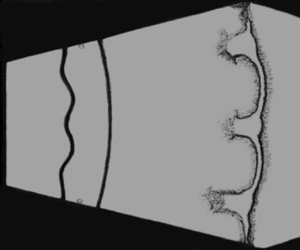
Developments of the wave patterns and interfacial morphologies for six cases are shown in figure 4. Since the evolution processes for these cases are qualitatively similar, we take case 2 as an example to detail the evolution process. At the beginning ( $-20\,\mathrm {\mu }$s), an incident cylindrical shock (ICS) together with the inner and outer interfaces of the gas layer can be clearly observed. The ICS has a cylindrical shape and also the inner (outer) interface presents an ideal single-mode (cylindrical) shape, which demonstrates good feasibility of the present experimental method. Later, ICS collides with the inner interface (air/SF $_6$), immediately bifurcating into a sine-like transmitted shock (TS $_1$) and a reflected shock (RS $_1$). During this process, the inner interface suffers a quick drop in amplitude due to shock compression. Later, driven by pressure disturbance and baroclinic vorticity, the amplitude of the inner interface increases persistently before the arrival of the rarefaction wave (RW $_1$). Subsequently, the disturbed TS $_1$ encounters the outer interface, generating a second transmitted shock (TS $_2$) that has a larger amplitude than TS $_1$. It indicates that the outer interface (SF $_6$/air) here serves as an ‘amplifier’ for the perturbation amplitude of a passing shock. During this process, TS $_1$ seeds a small positive perturbation on the outer interface. In this work, the amplitude of perturbation with the same phase as that of the inner interface is defined as positive, and otherwise negative. As time proceeds, TS $_2$ propagates downwards with its amplitude decaying gradually and finally recovers to a uniform cylindrical shock. To clearly show the layer evolution process, sketches of the wave patterns and interfacial morphologies at typical moments for case 2 are given in figure 5. In the following two subsections, we quantitatively discuss the instability growths at the inner and outer interfaces, respectively.

Figure 4. Schlieren images showing the developments of wave patterns and interfacial morphologies for all cases. ICS denotes the incident cylindrical shock and II $_1$ is the initial first interface. The other symbols are the same as those in figure 2. The numbers are in $\mathrm {\mu }$s.

Figure 5. Sketches of the wave patterns and interface morphologies at typical moments for case 2. Here,  $\Delta V_2$ ( $\Delta V_2^*$) is the velocity of the outer interface after the impact of TS $_1$ (CW $_1$). The other symbols are the same as those in figure 4. The numbers are in $\mathrm {\mu }$s.
3.2.1. Instability growth at the inner interface
Normalized variations of the amplitude of the inner interface versus time for all cases are plotted in figure 6. The interface amplitude is normalized as  $\alpha = n(a_1- a_1^+ ) / R_{01}$ and the time as $\tau =n\dot {a}_0(t-t_1^+ )/ R_{01}$. Here, $a_1^+$ refers to the post-shock amplitude of the inner interface and $t_1^+$ to the time just after the incident shock passes across the inner interface, and $\dot {a}_0$ denotes the perturbation growth rate shortly after the shock impact, which can be obtained by a linear fit of experimental data, as listed in table 2. At the early stage, the dimensionless amplitude histories collapse quite well for all cases and also are in good agreement with the RM instability growth at a single interface. When RW $_1$ interacts with the evolving inner interface, RT instability and interface stretching begin to play a role, causing a quick rise in perturbation growth rate. Later, the perturbation growth rate decays continuously with time. It is found that a thicker gas layer results in a larger extent that the RW $_1$ promotes the instability growth at the inner interface. For case 1 with a thinner gas layer, RW $_1$ arrives at the inner interface earlier and thus the interface presents a larger amplitude than thicker cases at the early stage. Nevertheless, at late stages, the inner interface presents a smaller perturbation amplitude than that of thicker layers. For cases 3–6, the perturbation growth rate approaches zero at late stages (i.e. the instability freezes out Mikaelian Reference Mikaelian1985). It can be generally found that the existence of the outer interface promotes the instability growth at the inner interface as compared to RM instability at an isolated single-mode interface (Li et al. Reference Li, Ding, Zhai, Si, Liu, Huang and Luo2020).

Figure 6. Normalized variations of the amplitude of the inner interface versus time for different cases. SI refers to the perturbation growth of a single air/SF $_6$ interface from Li et al. (Reference Li, Ding, Zhai, Si, Liu, Huang and Luo2020). The dashed line refers to the prediction of Bell model, the dash–dotted line to the prediction of the Bell-RT model, and the solid line to the prediction of the Bell-RT-m model that considers the interface stretching and RT instability caused by RW $_1$.
$_1$.
Table 2. The post-shock parameters for six cases. Note:  $t_{i}^{+}$ refers to the time just after the shock crosses the inner ( $i=1$) or outer ( $i=2$) interface; $a_{i}^{+}$ to the corresponding amplitude at $t_{i}^{+}$; $\Delta V_{i}$ to the post-shock velocity of the interface; $\dot {a}_{0}$ to the growth rate of the inner interface at $t_{i}^{+}$.

The instability growth at the inner interface can be generally divided into three stages: early stage, intermediate stage (i.e. wave interaction stage) and late stage. At the early stage ( $t< t_1^{RW}$), the perturbation growths for various-thickness layers collapse quite well, which indicates a negligible interface coupling effect. Thus, the instability growth at this stage can be described by the linear theory for cylindrical RM instability at an isolated interface. According to Bell (Reference Bell1951) and Ding et al. (Reference Ding, Si, Yang, Lu, Zhai and Luo2017b), the growth of cylindrical RM instability at a single-mode interface can be described as
 \begin{equation} \frac{1}{R^{2}} \frac{{\rm d}}{{\rm d} t}\left(R^{2} \dot {a} \right)-(n A-1) \frac{\ddot{R}}{R} a=0, \end{equation}
where  $\dot {a}$ is the first derivative of amplitude with time and $\ddot {R}$ is the second derivative of radius with time. Treating the shock impact as an impulse function (i.e. $\ddot {R} = \delta (t)\Delta V$), the perturbation amplitude at an arbitrary time $t$ can be obtained by integrating (3.13),
 \begin{equation} a(t)=a_{0}^{+}+\dot{a}_{0} R_{0}^{2} \int_{t_{0}^{+}}^{t} \frac{1}{R^{2}(t')} \,{\rm d} t'+(n A-1) \int_{t_{0}^{+}}^{t}\left(\frac{1}{R^{2}(t')} \int_{t_{0}^{+}}^{t'} a R \ddot{R} \,{\rm d} t^{''}\right) \,{\rm d}t'. \end{equation}
Here,  $t_0^+$ refers to the time just after the shock passage and $\dot {a}_0$ to the initial growth rate at $t_0^+$, which can be obtained by a linear fit of experimental data (shown in table 2). The first term on the right-hand side of (3.14) stands for the post-shock amplitude, the second term for pure RM instability combined with the geometric divergence effect and the third term for the perturbation growth associated with RT instability/stability. For brevity, (3.14) is termed as the Bell-RT model. Dynamics of an unperturbed gas layer in § 3.1 shows that the inner interface moves at a constant speed at the early stage. For this situation, the third term equals zero and (3.14) is called the Bell model. As shown in figure 6(a), the Bell model gives a reasonable prediction of the perturbation growth at the early stage for all cases. This further confirms that the interface coupling effect is very weak at the early stage.
At the intermediate stage, RW $_1$ accelerates the inner interface and thus the Bell model deviates from the experimental results. We realise that RW $_1$ does not only accelerate but also stretches the inner interface. In the following analysis, we take both RT instability (caused by interface acceleration) and interface stretching into account. First, we consider the stretching effect. Since the interface stretching process lasts for a short period of time, during which the interface travels a short distance, this process can be approximately considered as that happening in a planar geometry. This approximation can simplify the analysis. As sketched in figure 7, RW $_1$ first crosses the peak of the inner interface (point A), causing a local velocity rise, whereas the trough of the interface (point B) moves at its original speed before the arrival of RW $_1$. Such a velocity difference produces a quick increment in interface amplitude, which is termed as the stretching effect. The stretching process involves three phases: RW $_1$ passes across point A ( $t_{1}^{RW}$ $\sim$ $t_{2}^{RW}$), RW $_1$ tail leaves point A but its head has not arrived at point B ( $t_{2}^{RW}$ $\sim$ $t_{3}^{RW}$), and RW $_1$ passes across point B ( $t_{3}^{RW}$ $\sim$ $t_{4}^{RW}$). Time duration for the first phase is $\Delta t_1=t_{2}^{RW}-t_{1}^{RW}$, for the second phase is $\Delta t_2=t_{3}^{RW}-t_{2}^{RW}$, and for the third phase is $\Delta t_3=t_{4}^{RW}-t_{3}^{RW}$. Obviously, there is $\Delta t_1=\Delta t_3$.

Figure 7. Sketches showing the interface stretching process by rarefaction wave RW $_1$.
$_1$.
To simplify the analysis, we assume the interface undergoes a constant acceleration ( $g$) during the passage of RW $_1$. The constant acceleration is $g=(\Delta V_1^*-\Delta V_1)/\Delta t_1$, which can be estimated by the 1-D theory developed in § 3.1. The layer thickness at the time when TS $_1$ encounters the outer interface is denoted by $d^*$, which can be readily obtained. Also, the width of RW $_1$ (defined as the distance between its head and tail) at the moment when it encounters the inner interface is $L=(\gamma + 1)(\Delta V_2 - \Delta V_1)d^* / (2c)$, where $\gamma$ and $c$ denote the specific heat ratio and sound speed behind TS $_1$ inside the gas layer, respectively. For the first/third phase, the interface motion satisfies $g(\Delta t_1)^2/2+c\Delta t_1=L$. Combining the above equations, $\Delta t_1$ and $g$ can be readily calculated. For the second phase, there is $c\Delta t_2 =2a_1^*-c\Delta t_1$, where $a_1^*$ is the amplitude of the inner interface immediately before the impact of RW $_1$. Analytical solutions for the key parameters are summarized as
 \begin{equation} \left. \begin{gathered} \Delta t_{1}=\Delta t_{3}=2 L /\left(2 c+\Delta V_{1}^{*}-\Delta V_{1}\right), \\ \Delta t_{2}=\left(2 a_{1}^{*}-c\Delta t_1\right) / c, \\ g=\left(\Delta V_{1}^{*}-\Delta V_{1}\right) / \Delta t_{1}. \end{gathered} \right\} \end{equation}
The above parameters are calculated and listed in table 3. With these values, the displacement difference between points A and B at the stretching stage is
 \begin{equation} \Delta x=(\Delta V_{1}^{*}-\Delta V_{1})(\Delta t_{1}+\Delta t_{2}). \end{equation}
Thus, the average growth rate caused by interface stretching is
 \begin{equation} \dot{a}_s=\Delta x/[2(\Delta t_1 + \Delta t_2 + \Delta t_3)]. \end{equation}
Table 3. The relevant parameters for cases 1–6. Note:  $a_{1}^{*}$ is the inner interface amplitude just before the arrival of RW $_1$;
$_1$;  $d^{*}$ is the layer thickness at the time when TS $_1$ encounters the outer interface; $L$ is the width between the head and tail of RW $_1$ when it arrives at the inner interface; $\Delta V_1^*$ is the velocity of the inner interface after the impact of RW $_1$;
$_1$;  $\Delta t_{1}$ ( $\Delta t_{2}$) is the time of the first (second) stage for RW $_1$ interacting with the perturbed inner interface; $g$ is the acceleration of the inner interface caused by RW $_1$; and $\dot {a}_{s}$ is the average growth rate caused by interface stretching.

Next, we consider the effect of RT instability caused by RW $_1$ on the perturbation growth by incorporating the average acceleration $g$ calculated by (3.15) into the Bell-RT model. Finally, a modified Bell-RT model (Bell-RT-m) accounting for both the RT effect and interface stretching can be proposed, which is written as
 \begin{gather} a(t)=a_{0}^{+}+\dot{a}_{0} R_{0}^{2} \int_{t_{0}^{+}}^{t} \frac{1}{R^{2}(t')} \,{\rm d} t'+(n A-1) \int_{t_{0}^{+}}^{t}\left(\frac{1}{R^{2}(t')} \int_{t_{0}^{+}}^{t'} a R \ddot{R} \,{\rm d} t^{''}\right) \,{\rm d}t' +\dot{a}_s (t-t_1^{RW}). \end{gather}
Note, (3.18) is valid only during the interaction of RW $_1$ with the inner interface (i.e. $t_1^{RW}< t< t_4^{RW}$). As shown in figure 6, the Bell-RT-m model well reproduces the quick instability growth at the wave interaction stage for all cases, which demonstrates its validity. It is found that for cases with a thicker gas layer or a larger amplitude-to-wavelength ratio, RW $_1$ promotes the instability growth to a larger extent. This is also confirmed by the Bell-RT-m model. The reason is discussed below. As the layer thickness or the initial amplitude-to-wavelength ratio becomes larger, the interface amplitude experiences a longer period of linear growth or a faster linear growth. As a result, the inner interface possesses a larger amplitude just before the arrival of RW $_1$, giving rise to stronger RT and stretching effects. It is also found that RW $_1$ promotes the growth of divergent RM instability to a larger extent as compared to the planar counterpart (Liang & Luo Reference Liang and Luo2021a). This is ascribed to an overall slower growth of divergent RM instability caused by geometric expansion than the planar counterpart.
At late stages, reverberating waves inside the layer are negligibly weak and also the inner interface decelerates evidently due to geometric divergence, producing RT stability. Thus, the instability growth at the late stage is dominated by RM instability and RT stability. It has been reported by Li et al. (Reference Li, Ding, Zhai, Si, Liu, Huang and Luo2020) that for divergent RM instability at an isolated interface, nonlinearity is very weak and produces a negligible influence on the growth of overall amplitude. Hence, the linear Bell-RT model can be adopted to predict the growth of divergent RM instability at late stages. Here, we first calculate the interface deceleration according to the 1-D theory developed in § 3.1, and then substitute the calculated deceleration into the Bell-RT model. In this way, the Bell-RT model gives a good prediction of the perturbation growth for cases 1, 2 and 4, as shown in figure 6. Nevertheless, it fails to reproduce the very slow instability growth (even the instability freeze-out) after the impact of RW $_1$ for cases 3, 5 and 6. This is ascribed to relatively stronger nonlinearity in these cases in which the interface amplitude is quickly amplified by RW $_1$. It should be noted that for case 1 with a thin layer, the perturbation amplitude continues increasing after reaching saturation ( $\tau > 0.8$) due to the increasing interface coupling effect, which is not considered by the Bell-RT model.
3.2.2. Instability growth at the outer interface
Variations of the amplitude of the outer interface versus time for all cases are plotted in figure 8. Unlike the inner interface, the outer interface presents no perturbation initially. Thus, it is difficult to choose appropriate reference quantities for normalization. This is the reason why figure 8 is plotted in physical units. The perturbation growths for various-thicknesses cases are distinctly different. Specifically, for case 1 with a thin layer, the transmitted shock TS $_1$ presents a larger perturbation amplitude immediately before it encounters the outer interface (SF $_6$/air). Thus, a relatively larger perturbation is seeded at the outer interface by the rippled TS $_1$. As CW $_1$ impacts the outer interface, such a perturbation experiences a quick growth. At late stages, the perturbation amplitude continues growing due to interface coupling. Differently, for thicker gas layers (cases 2 and 3), TS $_1$ travels a longer distance to arrive at the outer interface and its amplitude undergoes a greater degree of decay during this process. As a consequence, only a subtle perturbation is produced at the outer interface by TS $_1$, even for case 5 with an initial larger perturbation at the inner interface. This differs greatly from convergent RM instability (Ding et al. Reference Ding, Li, Sun, Zhai and Luo2019), where the distorted transmitted shock keeps invariant or even increases in amplitude during the propagation process, and consequently seeds a considerably large perturbation at the downstream interface. Afterwards, the growth rate of the interface amplitude remains nearly zero before the arrival of CW $_1$ (i.e. freezes out). The reason for the instability freeze-out is given below. First, the uniform TS $_1$ in cases 2 and 3 produces no velocity perturbation, continuous pressure perturbation and baroclinic vorticity (i.e. there are no forces driving the instability growth). Second, even though there is a small perturbation produced by TS $_1$, its amplitude would reduce due to geometric divergence. Also, after CW $_1$ encounters the outer interface, the interface amplitude experiences a considerably quick growth. Later, as the two interfaces become closer to each other, the interface coupling effect becomes dominant, which continuously promotes the instability growth at the outer interface.

Figure 8. Variations of the amplitude of the outer interface versus time. The solid line refers to the model prediction considering the effect of CW $_1$ and interface coupling, the dashed line to model prediction considering interface coupling effect and the dash–dotted line to the prediction of (3.27).
The CW $_1$ and interface coupling are major factors driving the instability growth at the outer interface. Here, we first give a quantitative analysis on the effect of CW $_1$ on the instability growth. The mechanism for the perturbation growth induced by CW $_1$ is illustrated in figure 5. Considering the thickness of the gas layer is much smaller than its radius (i.e. $d \ll R$), waves inside the layer vary slightly in speed and thus can be assumed to be of constant strengths (Sun et al. Reference Sun, Ding, Zhai, Si and Luo2020). The velocity jump ( $\Delta V_{cw}\approx$ 8 m s $^{-1}$) of the outer interface caused by CW $_1$ for the unperturbed case can be adopted to approximate that of a perturbed layer. According to a simple analysis, the amplitude of the distorted CW $_1$ is found to be nearly twice the amplitude of the inner interface at the time when RW $_1$ encounters the inner interface ( $a_1^*$). Then, the time duration for the distorted CW $_1$ passing through the perturbed outer interface is $\Delta t_{cw}=(4a_1^*-2a_2^*) / c$, where $a_2^*$ is the amplitude of the outer interface just before its collision with CW $_1$. The calculated results for all cases are listed in table 4. Hence, the average growth rate of the outer interface caused by CW $_1$ is $\dot {a}_{cw}=\Delta V_{cw}/2$.
Table 4. The relevant parameters for the interaction between CW $_1$ and the outer interface. Note: $a_2^*$ is the perturbation amplitude of the outer interface just before the arrival of CW $_1$;
$_1$;  $\Delta t_{cw}$ is the duration for the perturbed CW $_1$ passing through the outer interface; $\beta$ is the coupling angle; and $\dot {a}_1^{cou}$ ( $\dot {a}_2^{cou}$) represents the growth rate of the inner (outer) interface.

After CW $_1$ moves away, the amplitude of the outer interface grows persistently. This is mainly ascribed to the interface coupling effect. For the evolution of a gas layer with two interfaces, Mikaelian (Reference Mikaelian1995) proposed a linear model (MIK model) to quantify the influence of interface coupling on the instability growth, which is written as
 \begin{equation} \left. \begin{gathered} \dot{a}^{cou}_{1} =\displaystyle\frac{\Delta V \varGamma^{2}}{\cos \beta}\left(a_{01}-a_{02} \sin \beta\right),\\ \dot{a}^{cou}_{2} ={-}\displaystyle\frac{\Delta V \varGamma^{2}}{\cos \beta}\left(a_{02}-a_{01} \sin \beta\right), \end{gathered} \right\} \end{equation}
where
 \begin{equation} \left. \begin{gathered} \varGamma^{2} \equiv k(D-1) /\left[1+D^{2}+2D \operatorname{coth}(k d)\right]^{1 / 2},\\ \sin \beta=\left(2 W_{1} / W_{2}\right) /\left[1+\left(W_{1} / W_{2}\right)^{2}\right], \\ W_{1} / W_{2}=1+S T+(S / D)\left\{ 1+\left[1+D^{2}+2D \operatorname{coth}(k d)\right]^{1 / 2} \right\}, D=\rho_{2} / \rho_{1}, \\ S \equiv \sinh (k d), \quad T \equiv \tanh (k d / 2). \end{gathered} \right\} \end{equation}
Here,  $a_{0i}$ and $\dot {a}^{cou}_i$ ( $i$=1 or 2 for the inner or outer interface) are the initial perturbation amplitude and perturbation growth rate, respectively, $k=n/R$ is the perturbation wave number, and $\Delta V$ is the velocity of the gas layer. When the layer thickness ( $d$) tends to infinity, the interface coupling angle ( $\beta$) that represents the strength of interface coupling tends to zero. Thus, (3.19) reduces to the impulsive model for each interface, i.e. the developments of the two interfaces are decoupled.
To clearly show the interface coupling effect on the growths of the inner and outer interfaces, we calculate the ratio of the growth rate predicted by the MIK model to impulsive model ( $\dot {a}^{SI}_{i}$),
 \begin{equation} \left. \begin{gathered} c_1=\displaystyle\frac{\dot{a}^{cou}_{1}(d)}{\dot{a}^{SI}_{1}}=\displaystyle\frac{\varGamma^{2}(d)}{\varGamma_{0}^{2}}\left(\frac{1}{\cos \beta}-\frac{a_{2}^{+}}{a_{1}^{+}} \tan \beta\right),\\ c_2=\displaystyle\frac{\dot{a}^{cou}_{2}(d)}{\dot{a}^{SI}_{2}}=\displaystyle\frac{\varGamma^{2}(d)}{\varGamma_{0}^{2}}\left(\frac{1}{\cos \beta}-\frac{a_{1}^{+}}{a_{2}^{+}} \tan \beta\right). \end{gathered} \right\} \end{equation}
Variations of  $c_1$ and $c_2$ with the layer thickness are plotted in figure 9. As we can see, for the present gas layer (inner interface is perturbed and outer interface is uniform), interface coupling produces a very weak influence on the inner interface development, but a significant influence on the outer interface. This reasonably explains the finding that the linear Bell model gives a good prediction of the inner perturbation development in experiment. According to (3.19), for $a_{02}=0$, the growth rate of the outer interface can be rewritten as
 \begin{equation} \dot{a}^{cou}_2 = \dot{a}^{cou}_1 \sin{\beta}. \end{equation}
Provided with the perturbation growth rate of the inner interface and the thickness of the unperturbed layer (measured from experiment), the growth rate of the outer interface can be obtained.

Figure 9. Variations of  $c_1$ and $c_2$ with the layer thickness.
Since nonlinearity is very weak for the divergent RM instability considered in this work, the growth rate of the outer interface can be obtained by a linear superposition of the two components caused by interface coupling and wave influence,
 \begin{equation} \dot a_2 = \dot a^{cw} + \dot{a}^{cou}_2 . \end{equation}
As shown in figure 8, (3.23) gives a reasonable prediction of the perturbation growth at the wave-affecting stage for all cases. After this stage ( $\dot a^{cw}=0$), the amplitude growth of the outer interface can also be well predicted by the model for cases 1–4. However, for cases 5 and 6, the model prediction deviates greatly from the experimental results. Specifically, at late stages the perturbation growth of the inner interface freezes out (i.e. the growth rate is zero), and thus the growth rate of the outer interface should be zero as indicated by (3.22). This is apparently inconsistent with the experimental observation. A major reason is that for cases 5 and 6, the amplitude of the inner interface is larger than the layer thickness at late stages (931, $902\,\mathrm {\mu }$s in figure 4), i.e. the two interfaces coalesce. For this situation, the original MIK model is invalid.
Here, a primary analysis based on the volume equivalence between perturbed and unperturbed layers is given. As found in § 3.1, when an unperturbed layer moves outwards, it becomes gradually thinner, which can be readily measured from experiment. We realize that the volume of a perturbed layer is equal to that of the unperturbed one during the motion process under the incompressible flow assumption. As sketched in figure 10, for a gas layer with a perturbed inner interface and an unperturbed outer interface, as the layer moves outward, the layer thickness decreases continuously. After a certain critical time ( $t^{cont}_0$) at which the amplitude of the inner interface is equal to the layer thickness, the bubble of the inner interface penetrates into the outer interface ( $t^{cont}_1$), forming a perturbation at the outer interface that has the same phase as the inner interface. Assuming the inner and outer interfaces are in the form of cosine perturbation at late stages, i.e.
 \begin{equation} \left. \begin{gathered} r_{1}=R_{1}-a_{1} \cos n \theta, \\ r_{2}=R_{2}-a_{2} \cos n \theta, \end{gathered} \right\} \end{equation}
where  $a_1$ ( $a_2$) is the amplitude of the inner (outer) interface, $R_2=R_1+a_1-a_2$, then the fluid area between the two perturbed interfaces is
 \begin{equation} S=\int_{-\theta_{0}}^{\theta_{0}} \,{\rm d} \theta \int_{r_{1}}^{r_{2}} r \,{\rm d} r=\left[\frac{3}{2} a_{2}^{2}-2\left(R_{1}+a_{1}\right) a_{2}+2 R_{1} a_{1}+\frac{1}{2} a_{1}^{2}\right]\theta_0, \end{equation}
and the fluid area  $S^{\prime }$ contained in the corresponding undisturbed gas layer is
 \begin{equation} S^{\prime}=\int_{-\theta_{0}}^{\theta_{0}} \,{\rm d} \theta \int_{R_{1}}^{R_{1}+d} r \,{\rm d} r=\left(2 R_{1} d+d^{2}\right) \theta_{0}. \end{equation}
For the perturbed and unperturbed cases, their areas should be equal at an arbitrary time. By combining (3.25) and (3.26), the relationship between the amplitude of the outer interface  $a_2$ and the amplitude of the inner interface $a_1$ can be obtained as
 \begin{equation} a_{2}=\frac{2\left(R_{1}+a_{1}\right)-\sqrt{6\left(R_{1}+d\right)^{2} -2\left(R_{1}+a_{1}\right)^{2}+3 a_{1}^{2}}}{3}. \end{equation}
Equation (3.27) indicates that as the amplitude of the inner interface becomes larger than the layer thickness, it greatly increases the outer perturbation development. To the best of the authors’ knowledge, such a perturbation growth that exists uniquely in divergent multi-layer RM instability is reported for the first time. For cases 1, 5 and 6, where the layer thickness is smaller than the amplitude of the inner interface, substituting the amplitude and radius of the inner interface as well as the layer thickness (obtained from experiment) into (3.27), the amplitude growth of the outer interface at late stages is obtained. As shown in figure 8, (3.27) gives a reasonable prediction of the late-stage instability growth at the outer interface for these three cases. This indicates that interface coupling plays a crucial role in the development of the outer interface at late stages although it produces a much weaker effect on the development of the inner interface. It should be mentioned that the present study is mainly focused on the RM instability induced by a weak shock. For the strong shock case, a compressibility effect becomes evident, producing possibly new flow structures and phenomena (Ranjan et al. Reference Ranjan, Niederhaus, Motl, Anderson, Oakley and Bonazza2007, Reference Ranjan, Niederhaus, Oakley, Anderson, Bonazza and Greenough2008).

Figure 10. Schematic diagrams showing the gas layer deformation for unperturbed and perturbed cases.
4. Conclusions
Experiments of divergent RM instability at a perturbed heavy gas layer (a sinusoidal inner interface and a circular outer interface) are realized in a novel shock tube designed based on shock dynamics theory. An existing soap-film technique is extended to generate gas layers with controllable shape and thickness. The dynamics of an unperturbed gas layer is first examined. It is found that differing from the layer motion in planar and convergent geometries, the gas layer in divergent geometry becomes increasingly thinner with time. The inner and outer interfaces of the layer move uniformly at the early stage and decelerate evidently at late stages. A general 1-D theory that takes the influences of waves and post-shock non-uniform pressure field into account is established, which gives a good prediction of the layer motion in divergent geometry from early to late stages.
Six types of perturbed SF $_6$ layers with different thicknesses and shapes surrounded by air are then considered. High-quality schlieren images are obtained, which clearly reveal the wave evolution and interface deformation. The instability growth at the inner interface involves three stages: early stage, intermediate stage and late stage. At the early stage, the perturbation growths for various-thickness layers collapse quite well, which indicates a negligible interface coupling effect. Thus, the Bell model for cylindrical RM instability at an isolated interface can be adopted to describe the perturbation growth. At the intermediate stage (i.e. during the interaction of RW $_1$ with inner interface), the perturbation growth rate experiences a quick rise due to the presence of RT instability and interface stretching. A modified Bell-RT model accounting for both RT instability and interface stretching is established, which well reproduces the quick instability growth at this stage for all cases. Both theoretical prediction and experimental result indicate that a thicker gas layer results in the larger extent that RW $_1$ promotes the instability growth. It is also found that RW $_1$ promotes the growth of divergent RM instability to a larger extent than the planar counterpart (Liang & Luo Reference Liang and Luo2021a) due to the overall slower growth of divergent RM instability caused by geometric expansion. At late stages, reverberating waves inside the layer are negligibly weak and the instability growth is dominated by RM instability and RT stability. For cases with strong nonlinearity, the instability nearly freezes out at the late stage, which is ascribed to the counteraction between the positive growth associated with RM instability and the negative growth associated with geometric divergence and RT stability.
Compression wave CW $_1$ and interface coupling are major factors driving the instability growth at the outer interface. As the distorted transmitted shock TS $_1$ passes across the uniform outer interface, it seeds a small perturbation at the outer interface. This seeded perturbation is smaller than the counterpart in planar and convergent geometries because the amplitude of TS $_1$ decays more quickly in divergent geometry. Then, the outer interface amplitude remains nearly invariant until the arrival of CW $_1$. As CW $_1$ encounters the outer interface, the interface amplitude experiences a quick growth. Later, as the two interfaces become close to each other, interface coupling effect becomes dominant, significantly promoting the development of the outer interface. A modified MIK model (Mikaelian Reference Mikaelian1995) that takes the influences of CW $_1$ and interface coupling into account is developed, which gives a good prediction of the instability growth. For cases where the inner interface amplitude is larger than the layer thickness, a new interface coupling mechanism that exists uniquely in divergent geometry dominates the development of the outer interface. The finding in this work provides deep insights into divergent RM instability at multiple interfaces, which is useful for understanding the hydrodynamic instabilities in ICF and supernova explosion.
Funding
This work was supported by the National Natural Science Foundation of China (nos. 12122213, 12072341, 91952205 and 12027801).
Declaration of interests
The authors report no conflict of interest.


