


Introduction
Coaxial comb-line resonator bandpass filters are analog key components of current and future communication systems. They are frequently used in e.g. base-stations due to the good relation between manufacturing costs, achievable Q-factor and their robustness [Reference Höft, Burger, Magath and Bartz1]. The rapid evolution of analog front-end components requires a targeted development of filters. Therefore, it is meaningful to use a completely modular filter platform in which different components like input-/output- and cross-couplings, as well as variable filter topologies, can be tested before they are used in a fabricated filter. Furthermore, the set-up is best suited for education purposes.
The proposed filter platform is completely modular and is in the current configuration able to realize up to 11 coupled coaxial resonators, whereby an extension to higher filter orders is easily possible by using a larger ground plate/cover. The platform is only composed by a top and a bottom plate separated by commercially available low-cost PCB (printed circuit board) spacers in between (also denoted as “posts”), building the enclosure of each cavity. Six PCB spacers in the middle of each cavity are used to implement the inner conductor. The modularity and versatility of the filter is shown within this paper, which is organized as follows:
In the section “Filter set-up” the basic filter set-up and components are described in detail. The section “Input-/output- and cross-couplings” provides an overview on a large variety of input-/output- and cross-couplings available for the proposed filter platform. Subsequently, the section “Filter topologies and reconfiguration of the comb-line filter” summarizes standard filter coupling topologies which can easily be realized with the proposed filter. Finally, the section “Diplexer” focuses on the realization of a diplexer in two ways: In the first configuration a T-junction is used while in the second configuration the separation of both signals takes place within a common resonator, which is an elegant solution if the center frequencies of both filters are very close to each other [Reference Macchiarella and Tamiazzo2,Reference Macchiarella and Tamiazzo3]. An extension to a triplexer configuration is theoretically possible as well [Reference Macchiarella and Tamiazzo4].
Filter set-up
The basic filter set-up is shown in Fig. 1, where currently an all-pole filter is realized by four honeycombed resonators. The honeycomb-structure is similar to the one proposed in [Reference Qiu, Wu, Xie, Yin and Mao5]. As the filter is enclosed between two plates separated by commercially available PCB spacers, it is in general similar to commonly known substrate integrated waveguide (SIW)-filters [Reference Ho, Li and Chen6], while here six additional rods with shorter length are used for realizing an inner conductor.
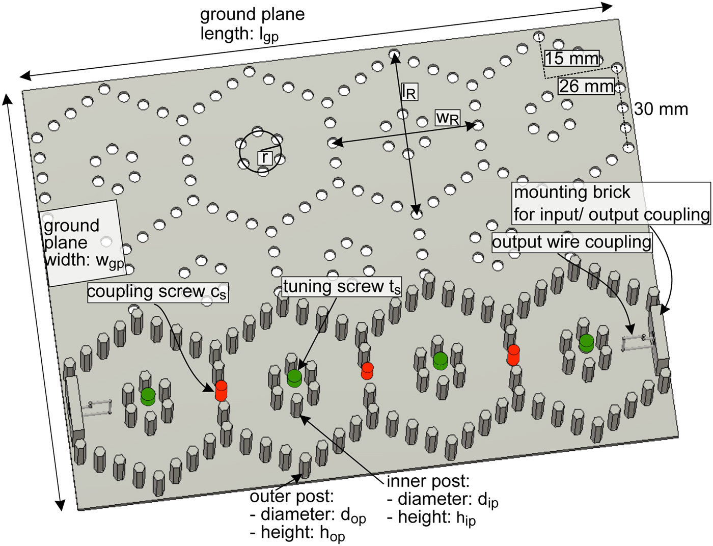
Fig. 1. Basic filter set-up consisting of a ground plate (w gp = 156 mm, l gp = 214 mm, and thickness = 2.5 mm) and PCB spacers, realizing currently a fourth order all-pole filter. The outer conductor has a total length of l R = 60 mm and a width of w R = 52 mm. The inner posts are arranged on a circle with radius r = 15 mm. Diameter of outer and inner posts: d op = d ip = 5 mm. Different heights of posts in between 4 mm < h ip, h op < 20 mm are available.
The resonators are disposed between a ground plate and a cover with side length w gp = 156 mm × l gp = 214 mm which are both realized in brass. The outer conductor of each resonator has a length of l R = 60 mm and a width of w R = 52 mm (Fig. 1). The six rods of the inner conductor are arranged on a circle with radius r = 15 mm.
One resonator is composed by maximally 24 spacers. Different heights of the PCB spacers are available, ranging from 4 mm until 20 mm length. Combination of the rods to achieve intermediate sizes is also possible. Longer rods are commercially available as well. An overview is shown in Fig. 2. To provide a good electrical contact between the ground plate and the cover, all spacers have an external thread on the lower side and an internal thread on the upper side. The achievable range of center frequencies for the outer post height ranging from 10 mm ≤ h op ≤ 30 mm and an inner post height of 5 mm ≤ h ip ≤ 29 mm is shown in the heat map in Fig. 3.
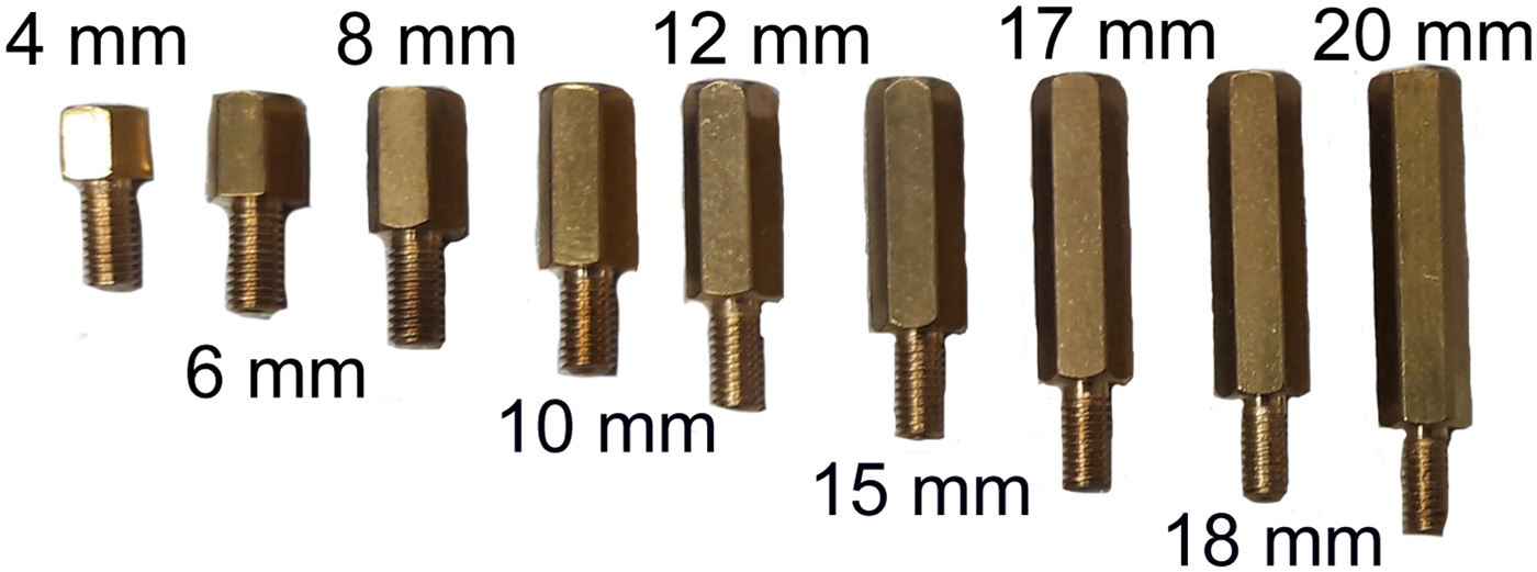
Fig. 2. Hexagonal rods (“PCB spacers”) with different available length manufactured in brass. All rods have a diameter of 5 mm, an external thread on the lower side and an internal thread on the upper side.
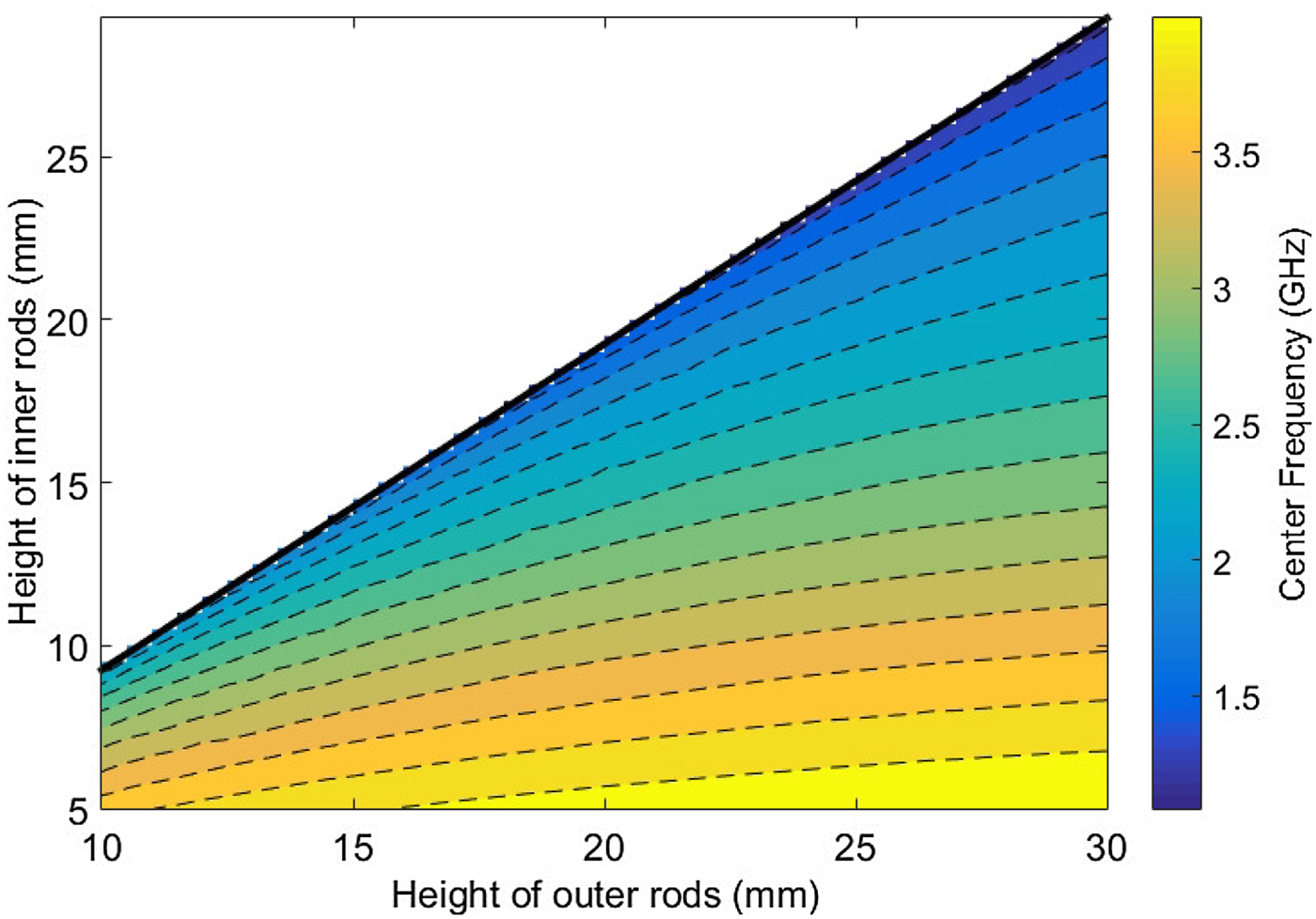
Fig. 3. Heat map for the achievable frequency range depending on the height of the inner and outer posts. The heat map is recorded without using tuning screws. Therefore, the frequency can further be degraded as shown in Fig. 4
Tuning of the center frequency is possible by M4 tuning screws t S (green screw in Fig. 1), which are mounted in the cover as well. The depth of the tuning screws can be varied during the measurement. Due to the nested structure of outer and inner conductor, as well as the tuning screw, the tuning range is comparably large [Reference Aouidad, Rius, Favennec, Clavet and Manchec7]. The tuning range for different heights of the inner conductor is shown in Fig. 4. To achieve the maximal possible Q-factor the height of the inner post should be chosen properly as each tuning screw screwed deep into the resonator increases the losses and reduces the Q-factor.
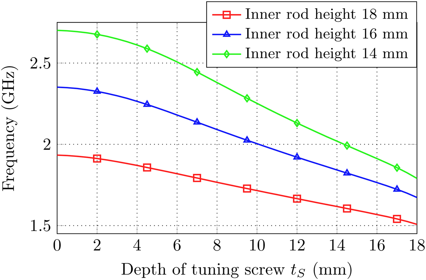
Fig. 4. Maximal tuning range for M4 tuning screws inserted in the cover for different heights of inner hexagonal rods and 20 mm outer rod height.
Couplings to adjacent resonators can be realized if one up to three hexagonal rods per coupling are omitted, which is possible at each edge of the honeycomb-structure (see Fig. 1). The spacer in the middle is replaced by a coupling-screw c S (red screw in Fig. 1), which is fixed with a threat in the cover (compare e.g. Fig. 6). The depth of the coupling screw can be varied within the tuning process. The number of spacers removed should depend on the desired bandwidth. In the standard configuration one coupling screw with two adjacent spacers is used, which ease the tuning process. In this case, the maximal bandwidth provided by the inter-resonator couplings is limited to B ≈ 25 MHz at 2 GHz. Fig. 5 shows the achievable non-normalized coupling factor in dependence of the depth of the coupling screw c S for the standard configuration and if two or three hexagonal rods are omitted. The coupling factor is calculated by
 $$ m_{ij} = {\displaystyle{\,f_{2}^{2}-f_{1}^{2}} \over {\,f_{2}^{2}+f_{1}^{2}}}, $$
where f i is the i-th eigenmode of a substructure containing two cavities and one coupling aperture in between [Reference Hong and Lancaster8]. If all hexagonal rods are omitted the maximal bandwidth can be enlarged to around 110 MHz at 2 GHz center frequency. Fig. 6 shows a realized sixth order filter with a cross-coupling between resonator 2 and 5. Please note that the distance between two hexagonal rods is 7.5 mm while each spacer has a diameter of around 5 mm. Therefore, the free space between two spacers is limited to 2.5 mm, which is much smaller than the wavelength at the center frequency of the filter, which is usually set to f 0 ≈ 2 GHz (λ0 ≈ 15 mm). Thus, an unwanted leakage of fields between the cavities and therefore an undesired coupling is avoided.
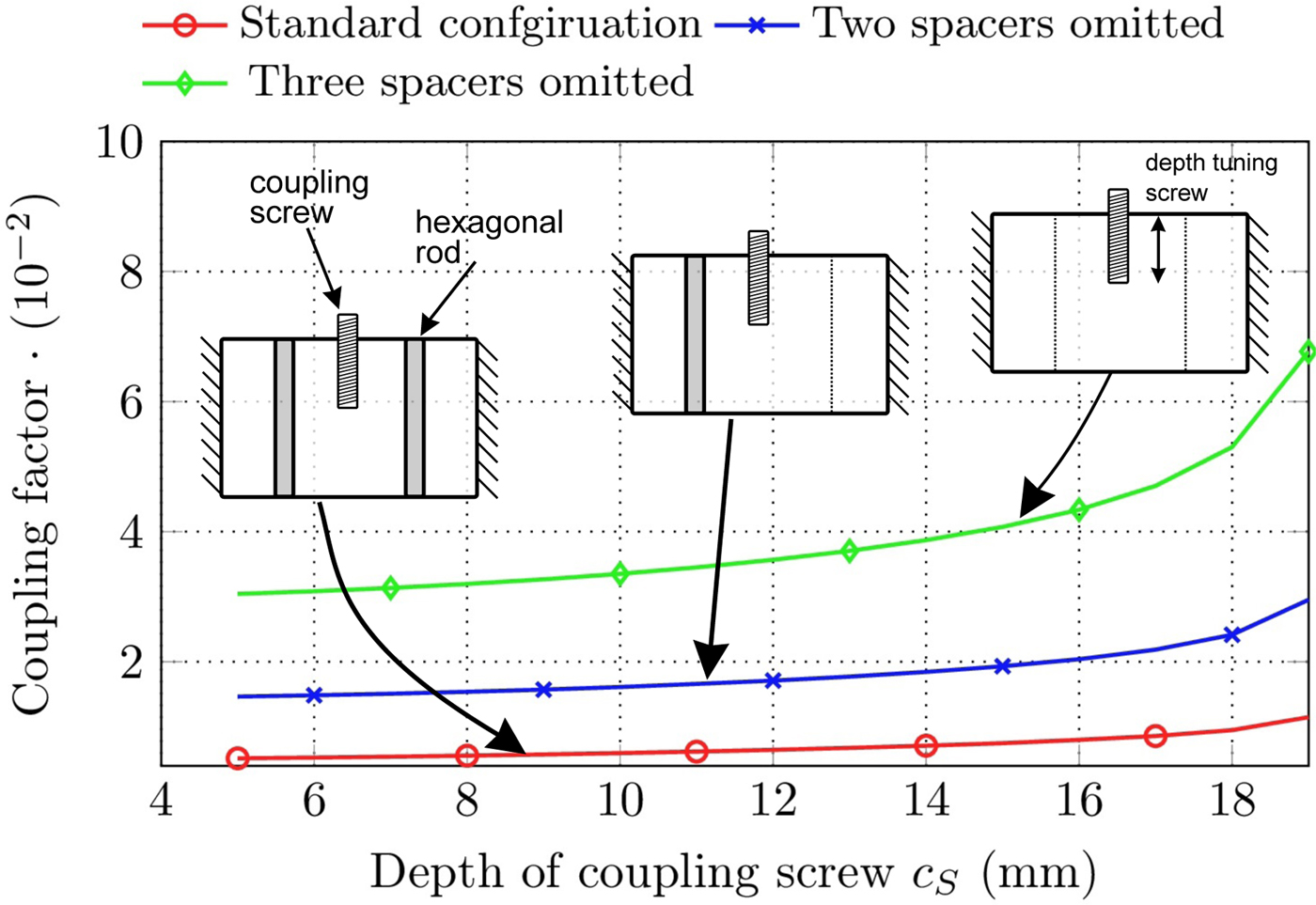
Fig. 5. Coupling factor in dependency of the depth of the tuning screw c S for the standard aperture and two up to three hexagonal rods omitted (height of the outer post is h op = 20 mm).
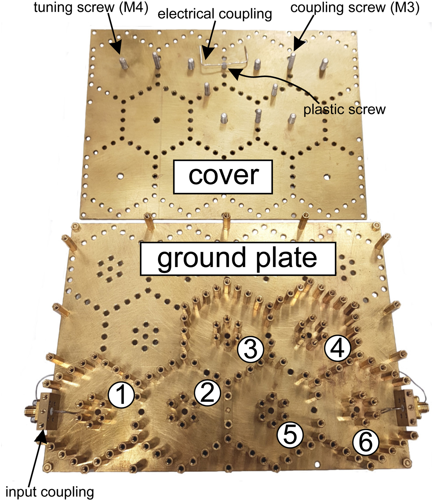
Fig. 6. Set-up of a sixth order folded filter with a pair of symmetric real frequency axis TZs. Cavity two and five are cross-coupled by a bended wire coupling in the cover, a bridge element is placed on the bottom plate. All tuning screws (M4) and coupling screws (M3) are mounted in the cover.
Input-/output- and cross-couplings
The modular structure of the proposed filter allows the integration of a wide class of input-/output- and cross-couplings. Figure 7 depicts a selection of input- and output-couplings. All of them are mounted on a brick of side length (20 mm × 20 mm × 5 mm), which can be positioned at every edge of each honeycomb resonator within the filter as shown in Figs 1 and 6.
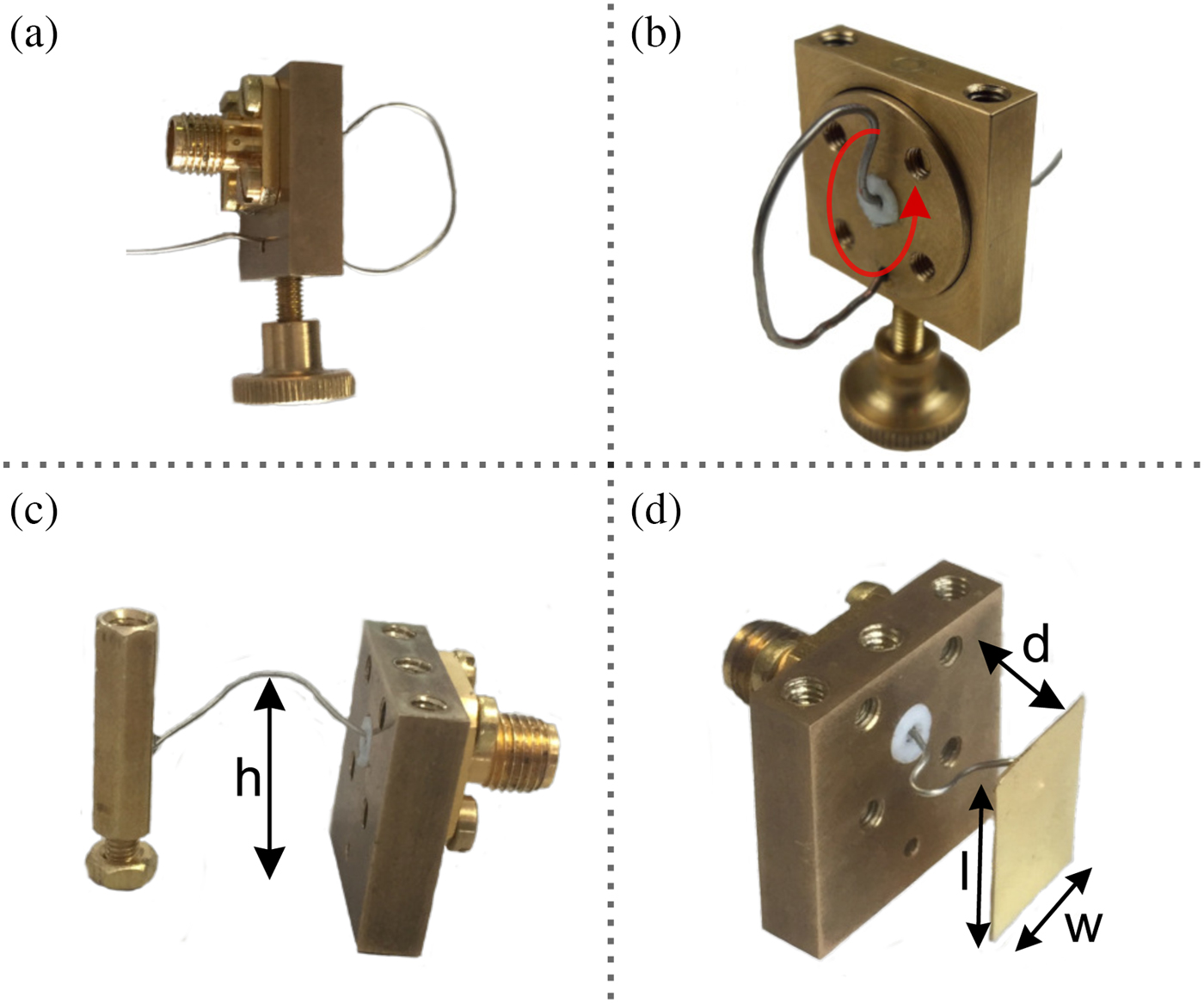
Fig. 7. Various input-couplings and maximal achievable bandwidth (at f 0 ≈ 2 GHz): (a) loop coupling, B max ≈ 18 MHz, (b) rotatable input coupling with assembled wire, (c) soldered wire coupling with moderate bandwidth. The maximal bandwidth strongly depends on the height, at which the wire is soldered on the inner post. (d) plate coupling, which achieves the highest possible bandwidth among the input couplings is proposed here (B max ≈ 110 MHz)
Figure 7(a) shows an inductive loop input-coupling which is built by simply bending a wire. The end of the wire is fixed by a knurled screw on the bottom of the brick. Loosen the screw allows subsequent tuning of the wire length by pulling and pushing the wire in the input-/output cavity. A large disadvantage of most input-couplings is the bad handling in terms of tunability, especially if small deviations must be compensated. One elegant solution is shown in Fig. 7(b). Here the inner part of the brick of Fig. 7(a) is manufactured as a rotatable cylinder. The coupling strength of the wire coupling of Fig. 7(a) mainly depends on the effective area of the loop which is perpendicular to the magnetic fields in the cavity. Therefore, rotating the inner cylinder and likewise the wire loop reduces the input-coupling strength.
Additionally, Fig. 7(c) shows the so-called wire coupling, where a wire with 0.8 mm diameter is soldered on the nearest inner post of the first or last cavity. Depending on the position at which the wire is soldered on the inner post, different coupling strengths can be achieved. Positions near the ground plane realize smaller values of the input-coupling strength. Changing the coupling strength after the wire is soldered on the inner post is possible by adapting the height h of the wire. Larger values of h lead to stronger input-couplings.
Finally, Fig. 7(d) depicts the plate-coupling which provides the maximal achievable input-coupling strength and hence bandwidth. In comparison to the input couplings of Figs 7(a) and 7(c), the plate-coupling is capacitive. The coupling strength is adapted beforehand by the width w and length l of the plate. After assembling the filter the input coupling strength can be varied by changing the distance d between the brick and the plate. Large values of d lead to higher coupling strengths.
It is worth to mention that also the couplings of Figs 7(c) and 7(d) can be mounted on the rotatable cylinder of Fig. 7(b) which might ease the tuning process.
In addition to various types of input-couplings, a variety of cross-couplings can be realized by the proposed filter as well. The filter can realize magnetic (“positive”) cross-couplings simply by coupling the desired cavities, like in the case of mainline couplings. Therefore,transmission zeros (TZs) above the passband in the case of triplets and complex pairs for phase equalization in the case of a quadruplet can easily be realized [Reference Cameron, Kudsia and Mansour9]. The coupling strength is adapted by inserting a standard M3 coupling screw in the cover in the direction of the ground plate [Reference Thomas10]. If TZs far away from the passband and hence weak cross-couplings are required, a bridge element as shown in Fig. 8 can be inserted. The bridge reduces the effective area at which mainly magnetic fields couple. In Fig. 8(b) the bridge is composed of three posts of 10 mm height, a small plate with 20 mm width, and 2 mm height as well as two further posts with 8 mm height. Other combinations are possible. The tuning takes place with a M3 tuning screw inserted from the cover of the filter.
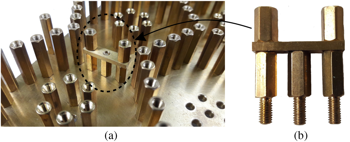
Fig. 8. “Bridge” element to reduce the coupling strength of magnetic fields: (a) mounted in the filter and (b) bridge element composed of six components.
For the realization of “negative” (in comparison to positive main path) couplings further commercially available material is needed.
Figures 9(a) and 9(b) depict the bended wire cross-coupling to realize a capacitive coupling. The wire is mounted on a plastic M3 screw, which is screwed in the cover before the filter is assembled. Depending on the horizontal length (l h) and the vertical depth (l v) the coarse coupling strength can be adjusted before the wire is mounted inside the filter. Fine tuning is subsequently possible by rotating the plastic screw in the assembled filter by the angle θ. To increase the absolute coupling strength the bridge element is mounted below the wire to reduce the magnetic fields within the coupling aperture [Reference Awai and Zhang11].
Fig. 9. Various cross-couplings: (a) bended wire coupling, (b) principle drawing of (a), (c) inverted-sign coupling, (d) principle drawing of (c), (e) electric plate coupling.
Figures 9(c) and 9(d) depict the inverted-sign coupling, which provides a negative coupling although it works inductive. It is composed of two bridge elements, one of which is placed on the top of the other by using two threaded rods. The magnetic field in the first cavity induces a current in the wire. Due to the bending, the current flows in the altered direction in the next cavity and generates a magnetic field in the opposite direction compared to the first cavity. The coupling is mounted on the three common rods of two adjacent cavities. Therefore, a negative magnetic coupling can easily be realized. The strength of the cross-coupling depends on the area surrounded by the wire in both cavities. This aperture was first proposed in [Reference Walker and Hunter12] for applications in dielectric TM-mode filters. A drawback of this cross-coupling is the bad tunability. A subsequent tuning is only possible by pushing or pulling the wire with a small tool, e.g. a screwdriver.
Finally, Figs 9(e) and 10 show a capacitive coupling realized by two plates, which are mounted on the inner conductor of two adjacent cavities. Please note that for the assembling the inner conductor must consist of two rods where the plate is clamped in between. The plates of length l p and distance h p to each other can be milled from a thin brass foil or cut out by using a tinsnips. The coupling strength depends on the length l p, width w p and the distance of both plates h p. Tuning of the cross-coupling in the assembled filter is possible by mounting a plastic screw in the cover, as depicted in Fig. 9(e). If the screw is turned down, the distance h p is reduced and the cross-coupling strength is enlarged. Please note that again a bridge element is additionally required to reduce the amount of coupled magnetic fields in the aperture.
Fig. 10. Close view on the electric plate coupling assembled in a filter.
The choice of the cross-coupling aperture depends on the necessary tunability and desired coupling strength.
Filter topologies and reconfiguration of the comb-line filter
Many standard coupling matrix topologies of up to eleventh order can be implemented by the proposed filter-platform. Higher order filters can be realized as well if further platforms are connected or rather the area of the ground and bottom plate is simply enlarged. An example of a sixth order folded filter with assembled rods realizing two real frequency axis TZs is already depicted in Fig. 6. In this example, the capacitive wire coupling is used for the realization of the negative cross-coupling between cavity 2 and 5. The wire is mounted in the cover by means of a plastic screw, which allows subsequent tuning. The measurement results are shown in Fig. 11. It is worth to mention that this cross-coupling is able to realize an asymmetry in the position of the associated TZs as well. If the wire is turned in the direction of cavity three, the total cross-coupling strength m 25 is reduced, otherwise, the coupling factor m 35 arises and the position of the TZs becomes slightly asymmetric. For this reason, one TZ above the passband is visible while the weaker TZ below is lost in the noise floor at approximately 1.648 GHz.
Fig. 11. S-Parameters and coupling diagram for the realization of a sixth order folded topology with two real frequency axis TZs.
Three further measurement results are depicted in the next figures. The associated filter topologies are depicted in each figure as well. Please note the following notation: Resonators are indicated with circles, nonresonating nodes (NRN) are represented by boxes, solid black lines indicate positive main-line couplings, dashed lines represent positive cross-couplings and negative cross-couplings are shown as dashed dotted (red) lines. The following topologies were realized for the proposed filter platform [Reference Cameron, Kudsia and Mansour9]:
• Sixth order folded topology with two TZs (already discussed in Fig. 11).
• Seventh order cascaded triplet topology with two TZs (Fig. 12).
• Fifth order cul-de-sac coupling matrix with two TZs (Fig. 13).
• Fourth order extracted pole topology with two TZs (Fig. 14).
Fig. 12. S-Parameters and coupling diagram for the realization of a seventh order triplet filter with two real frequency axis TZs.
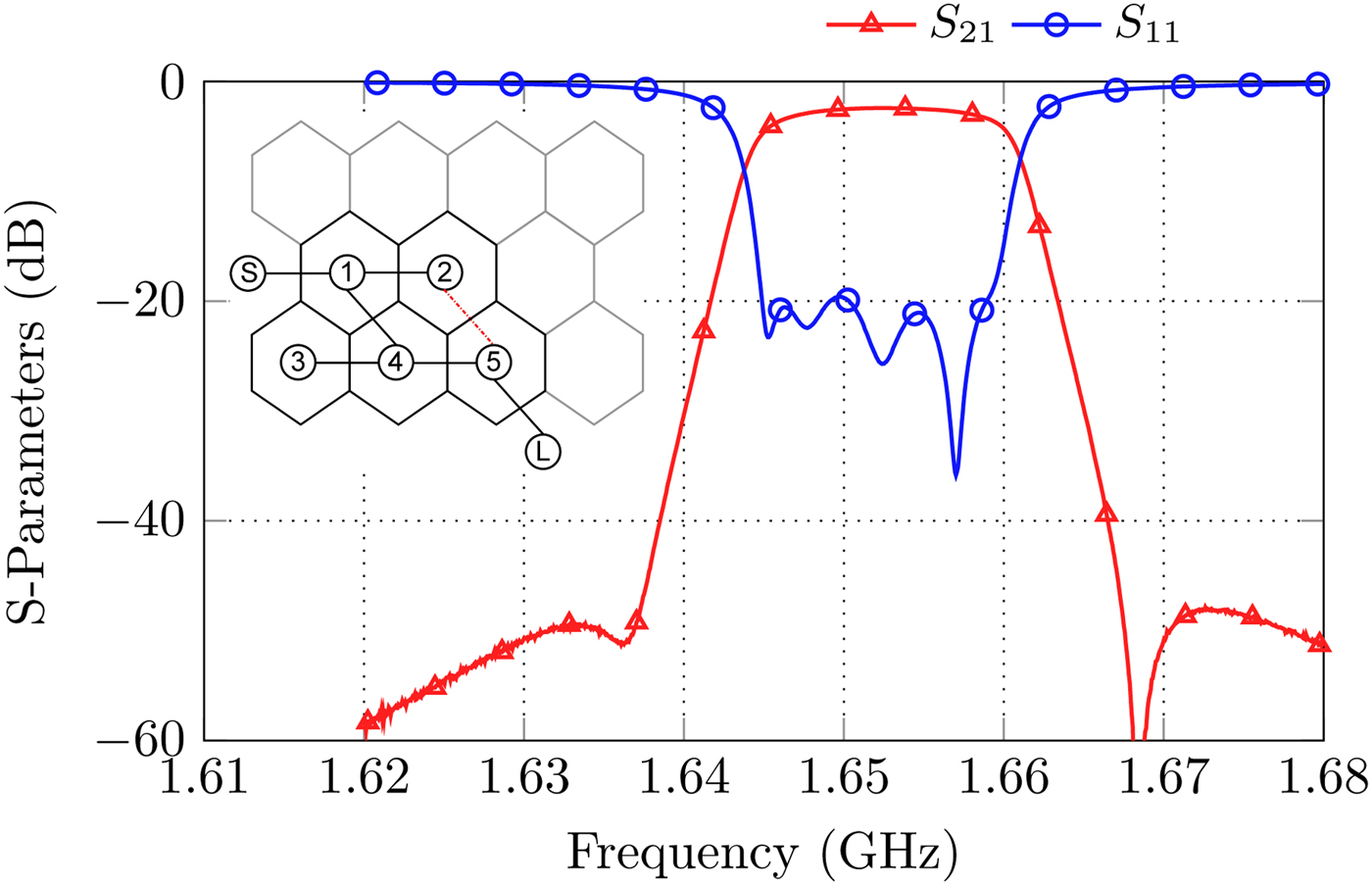
Fig. 13. S-Parameters and coupling diagram for the realization of a fifth order cul-de-sac filter with two real frequency axis TZs.
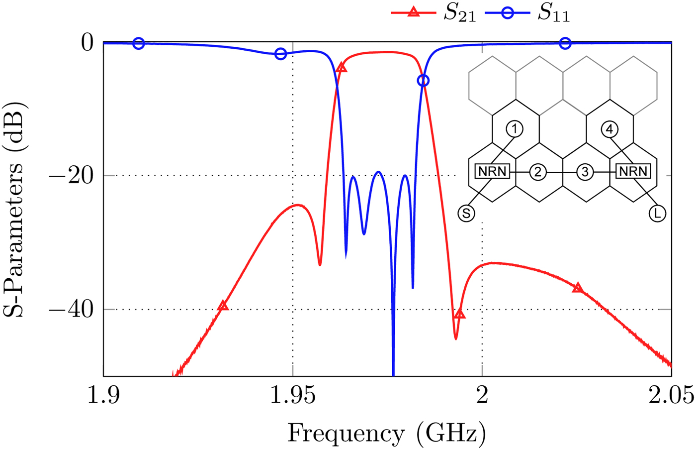
Fig. 14. S-Parameters and topology for the realization of a fourth order extracted pole filter. The extracted poles are connected to the main filter by nonresonating nodes.
For the first three examples the rotatable wire input-coupling was used, therefore the bandwidth is limited to around 18 MHz.
The versatility of the proposed filter is especially seen in the extracted pole filter of Fig. 14, which realizes two TZs without a need for a cross-coupling aperture. The coupling matrix was derived as proposed in [Reference Cameron, Kudsia and Mansour9,Reference Montejo-Garai, Ruiz-Cruz, Rebollar, Padilla-Cruz, Onoro-Navarro and Hidalgo-Carpintero13,Reference Amari and Macchiarella14]. Usually, the extracted pole cavities are coupled to the rest of the filter by NRNs, which can in many cases be designed as strongly detuned resonators or pieces of transmission lines of defined length [Reference Amari and Rosenberg15]. Within the honeycomb structure the NRNs can be realized by using a different inner post height compared to the “real” resonators which detunes them. A photograph of the set-up is shown in Fig. 15, the post heights used for this configuration are indicated in the caption. Please note that here the soldered wire input-coupling of Fig. 9(c) is used to provide a proper input-coupling strength. With this configuration a bandwidth of B ≈ 19 MHz is achieved.
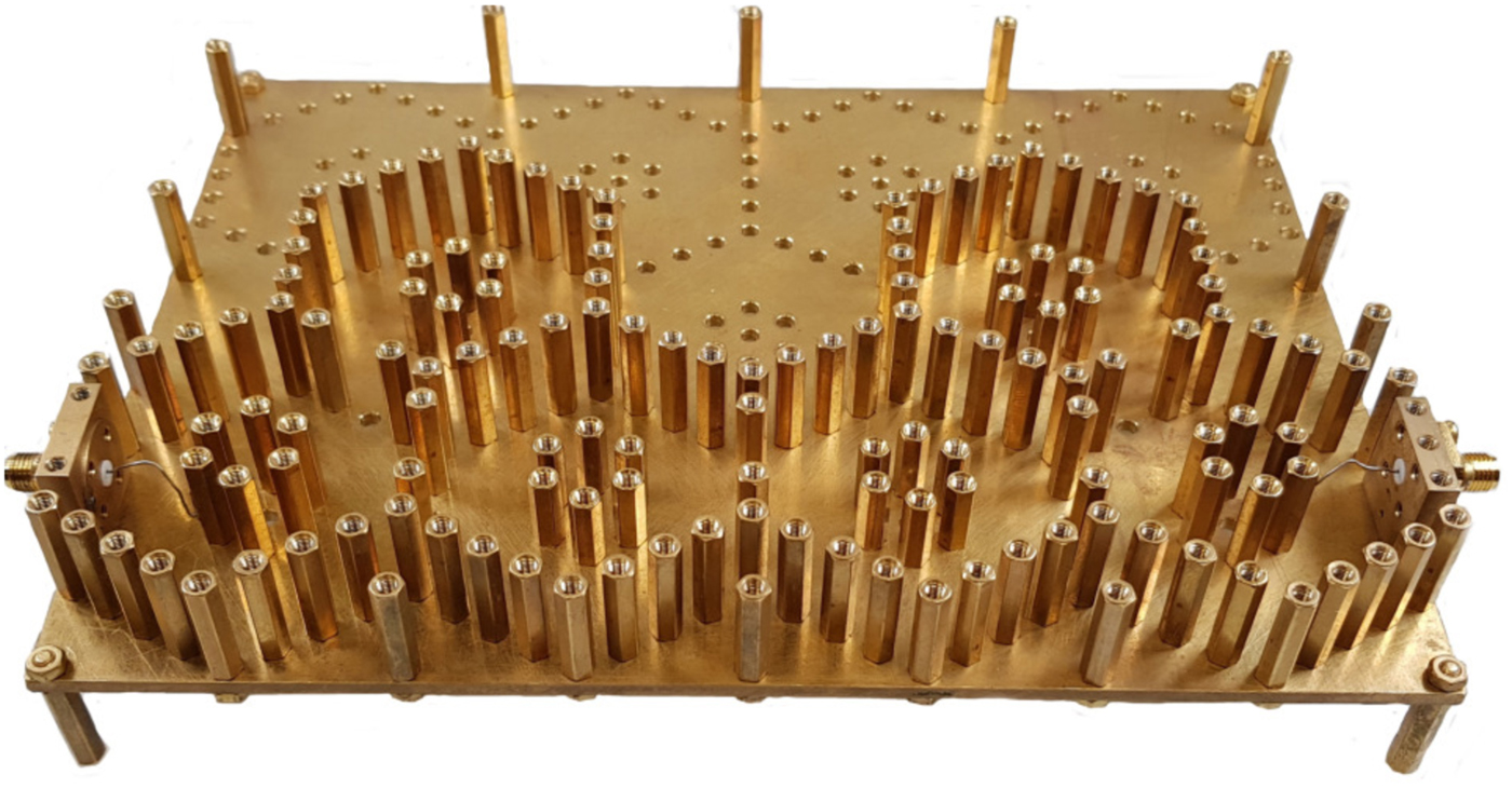
Fig. 15. Photograph of the filter set-up for the realization of a 4-2 extracted pole filter. For the nonresonating nodes inner posts with height h ip,NRN = 18 mm were used, all other posts of the inner conductor have a height of h ip,Res = 15 mm. The outer posts have a height of h op = 20 mm.
The Q-factor of all set-ups depends mainly on the depths of the tuning- and coupling screws. The deeper the screws are inserted, the lower is the Q-factor. Furthermore, all screws for mounting the cover and bottom plate should be tightened to reduce the losses. For the results proposed here the Q-factor was calculated in the range 1000 ≤ Q u ≤ 1300 [Reference Macchiarella16].
Diplexer
The proposed filter platform is best suited for the realization of diplexers. A diplexer consists of two bandpass filters with different center frequencies interconnected with each other realizing a three-port device. The filter with the higher center frequency is assumed here to be the TX filter while the other one is assumed to be the RX filter with the lower center frequency. The connection of both filters can be realized in two different ways. The choice of the connection method mainly depends on the frequency difference between the RX/TX passbands. If this difference is comparably large, both filters can be tuned independently and are connected afterwards using a splitting or T-junction. The length of the line between the T-junction and the input port of one filter is chosen in such a way, that the line transfers the impedance of the other filter to an open circuit at the center frequency of the first filter. The same is done for the second filter and the related center frequency. Both filters are tuned independently before they are connected with each other.
If the frequency offset is very small with respect to the center frequency, both filters should share a common resonator as proposed in [Reference Macchiarella and Tamiazzo3]. Here the overall size can be reduced since no transmission lines are needed while on the other hand the attenuation behavior is improved.
Shunt connected diplexer
The shunt connected type is explained by means of Fig. 16. One port of the T-junction is exemplary connected to a common antenna, while the further ports are connected to the TX and RX filters by means of transmission lines with length l i and phase constant βi. The aim of the following investigation is to find the length l i for fixed center frequencies of the TX and RX filters to achieve a minimal influence from the TX to the RX filter and vice versa. A simplified Smith chart of the problem is shown in Fig. 17.
Fig. 16. Connection of the TX and RX filter to a common T-junction with transmission lines of length l 1, l 2 and phase constants β1, β2.
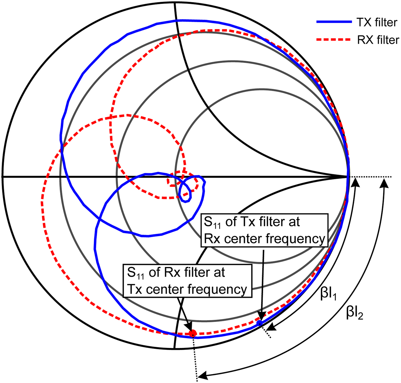
Fig. 17. Smith diagram of the individual TX and RX filters without additional transmission lines.
The length of the transmission line l 1 is chosen in that way that the TX filter is transformed to an open circuit at the RX center frequency. The length l 2 is calculated in the same way. The corresponding angular θi = l iβi can be gathered from the Smith chart.
Finally, Fig. 18 shows the results of a shunt connected diplexer consisting of two third order all-pole filters at 1.835 and 1.9 GHz. The method proposed in this section only allows the realization of diplexers with a relatively wide distance of the RX and TX center frequencies.
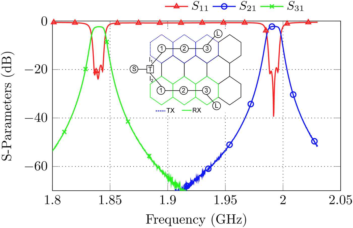
Fig. 18. S-Parameters and topology of the shunt-connected diplexer set-up.
Diplexer with common node
An elegant solution for the realization of diplexers with small frequency gap between the RX and TX path is the implementation of a common splitting resonator as proposed in [Reference Macchiarella and Tamiazzo3]. The advantages are an improved attenuation behavior as the filter order of the TX- and RX-filters is increased by one. Furthermore, the whole diplexer can be described by a coupling matrix, which ease the realization and tuning [Reference Macchiarella and Tamiazzo3]. The specifications for the RX filter are set to: filter order n RX = 3, one TZ above the passband at normalized frequency f TZ,RX = 2 and a return loss of RL RX = 20 dB while the TX filter is composed by four resonators (n TX = 4) and a minimal return loss of RL TX = 20 dB. The center frequency of the RX filter is chosen to be f 0,RX = 1.805 GHz with a bandwidth of B RX = 9 MHz while the TX filter is centered at f 0,TX = 1.82 GHz with a bandwidth of B TX = 9 MHz. Please note that the position of the normalized TZ of the RX filter is related to the RX center frequency. The corresponding coupling matrix is shown in (2). Tuning takes places by conventional coupling matrix extraction techniques using the Cauchy-method, which is extended for the application of diplexers in [Reference Traina17]. Fig. 19 finally shows the S-parameters and the coupling topology of the diplexer with common node, which is denoted as I. The matching of the diplexer implies some difficulties due to mutual influences between both filters. Considering the coupling matrix of (2) the following design constraints should be observed in the filter structure before the cover is assembled:
 $$\matrix{\hskip1.5pc S \hskip2.2pc I \hskip2.7pc 1 \hskip2.9pc 2 \hskip2.9pc 3 \hskip2.9pc 4 \hskip2.3pc L1 \hskip2pc 1 \hskip2.2pc 2 \hskip2.3pc 3 \hskip2.2pc L2 \cr \matrix{ S\cr I\cr 1\cr 2\cr 3\cr 4\cr L1\cr 1\cr 2\cr 3\cr L2} \left[\matrix{0 & 1.539 & 0 & 0 & 0 & 0 & 0 & 0 & 0 & 0 & 0 \cr 1.539 & 0 & 0.888 & 0 & 0 & 0 & 0 & 0.885 & 0 & 0 & 0 \cr 0 & 0.888 & -0.612 & 0.316 & 0 & 0 & 0 & 0 & 0 & 0 & 0 \cr 0 & 0 & 0.316 & -0.604 & 0.276 & 0 & 0 & 0 & 0 & 0 & 0 \cr 0 & 0 & 0 & 0.276 & -0.599 & 0.366 & 0 & 0 & 0 & 0 & 0 \cr 0 & 0 & 0 & 0 & 0.366 & -0.597 & 0.662 & 0 & 0 & 0 & 0 \cr 0 & 0 & 0 & 0 & 0 & 0.662 & 0 & 0 & 0 & 0 & 0 \cr 0 & 0.885 & 0 & 0 & 0 & 0 & 0 & 0.690 & 0.287 & 0.179 & 0 \cr 0 & 0 & 0 & 0 & 0 & 0 & 0 & 0.287 & 0.446 & 0.332 & 0 \cr 0 & 0 & 0 & 0 & 0 & 0 & 0 & 0.179 & 0.332 & 0.677 & 0.656 \cr 0 & 0 & 0 & 0 & 0 & 0 & 0 & 0 & 0 & 0.656 & 0}\right]} $$
• As the coupling between the source port and the common splitting resonator I is comparably high, a plate input coupling of Fig. 7 should be used.
• The coupling factor from the splitting resonator I to the first resonator of the TX/RX filters is much larger than the coupling factors within the individual filters. Therefore, the coupling should be realized with at least one hexagonal rod omitted (compare Fig. 5).
All other couplings can be implemented with one coupling screw or an inductive wire coupling of Fig. 7(a) for the two output ports.
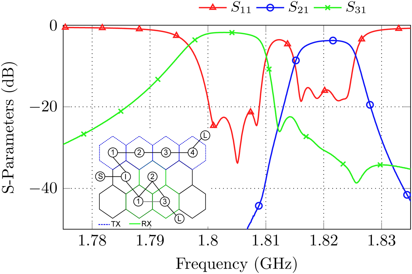
Fig. 19. S-Parameters and topology for the realization of a diplexer with common node.
Conclusion
A completely modular coaxial comb-line filter platform for prototyping and education purposes is presented. The function of different types of input-/output- as well as cross-couplings can be tested before the implementation into a fixed microwave filter set-up takes place. Within this paper, three different types of input couplings able to realize a wide variety of bandwidths with a large flexibility in terms of handling are proposed. Three types of cross-coupling apertures (positive and negative) are proposed as well.
Many of the commonly known canonical filter topologies like the folded form, the cul-de-sac form, cascaded triplets/quadruplets, as well as extracted pole filters, can easily be implemented with the modular filter platform. Furthermore, the proposed structure can be used for the realization of diplexers in two configurations. An extension to a triplexer is theoretically possible as well. Depending on the depth of all tuning screws, quality factors in the range of 1000 ≤ Q u ≤ 1300 can be achieved.
Author ORCIDs
Daniel Miek, 0000-0003-2452-5410; Michael Höft, 0000-0001-9352-2868
 Daniel Miek received the B.Sc. and M.Sc. degrees in electrical engineering and information technology from University of Kiel, Kiel, Germany in 2015 and 2017, respectively, where he is currently pursuing the Dr.-Ing. degree as a member of the Chair of Microwave Engineering with the Institute of Electrical Engineering and Information Technology.
His current research interest includes the design, realization, and optimization of microwave filters as well as parameter extraction and computer-aided tuning.
 Michael Höft was born in Lübeck, Germany, in 1972. He received the Dipl.-Ing. degree in electrical engineering and Dr.-Ing. degree from the Hamburg University of Technology, Hamburg, Germany, in 1997 and 2002, respectively.
From 2002 to 2013, he joined the Communications Laboratory, European Technology Center, Panasonic Industrial Devices Europe GmbH, Lüneburg, Germany. He was a Research Engineer and then Team Leader, where he had been engaged in research and development of microwave circuitry and components, particularly filters for cellular radio communications. From 2010 to 2013 he had also been a Group Leader for research and development of sensor and network devices. Since October 2013 he is a Full Professor at the Kiel University, Kiel, Germany in the Faculty of Engineering, where he is the Head of the Microwave Group of the Institute of Electrical and Information Engineering. His research interests include active and passive microwave components, (sub-) millimeter-wave quasi-optical techniques and circuitry, microwave and field measurement techniques, microwave filters, microwave sensors, as well as magnetic field sensors. Dr. Höft is a member of the European Microwave Association (EuMA), the association of German Engineers (VDI), a member of the German Institute of Electrical Engineers (VDE), and a senior member of IEEE.


 Open access