


I. INTRODUCTION
Modern digital technology bring miniaturization, low-power consumption, substantial computational power, and integration of complex processing on a small piece of silicon (system-on-chip). For modern radar systems, the full advantage of modern technology has been difficult to utilize in spite of faster devices and higher computational speed. As indicated in [Reference Browne1] modern radar systems are still fairly large modules with substantial size and power consumption.
The basic principles of radar have been known for more than a century, over the years several radar architectures have been explored; each with its own tradeoff in application and hardware complexity. Radar architectures differ mainly by the utilized waveform, example architectures contains, continuous-wave (CW) radar for velocity determination, pulsed ranging radar, frequency-modulated continuous-wave (FMCW) radar, stepped-frequency continuous-wave (SFCW) radar, and noise radar. The frequency-modulated architectures need a frequency source and a mixer, but require only a modest sampling rate of the mixer difference. The pulsed and noise radars are more amendable to digital implementation, but require a receiver that samples the entire transmitted bandwidth.
Several integrated radar systems have appeared in the literature, some with commercial interest. The first single-chip complementary metal–oxide–semiconductor (CMOS) radar was published by Hjortland et al. [Reference Hjortland, Wisland, Lande, Limbodal and Meisal2] in 2006, featuring a pulsed radar system now commercially available from Novelda [3]. Later an integrated SFCW radar was reported in 65 nm CMOS by Caruso [Reference Caruso, Bassi, Bevilacqua and Neviani4] for breast cancer detection. Sachs [Reference Sachs5] has written extensively on a M-sequence radar using SiGe BiCMOS technology. A growing application is automotive radars in the 60/70 GHz bands, where multiple single-chip solutions have been presented and some are commercially available [Reference Gresham6], CMOS realizations in the literature include [Reference Mitomo, Ono, Hoshino, Yoshihara, Watanabe and Seto7–Reference Guermandi10]. Several short-range radar systems are reported [Reference Lv, Dong, Sun, Li and Ran11–Reference Kuo13] indicating a number of potential sensing applications provided a compact, low-power, and high-performance radar is available; preferably in low-cost standard technology.
Figure 1 shows the proposed generic, programable system-on-chip radar with a FMCW receiver. Other architectures like CW, SFCW, as well as noise radar will be explained later in the paper, by simply replacing the dashed receiver circuit.

Fig. 1. Principle of a bitstream waveform generator utilized in a digital FMCW radar with a swept threshold receiver. The range spectrum is obtained after sampling, averaging and a frequency transform. Harmonics not shown, two up-sweeps depicted with different threshold levels for each sweep [Reference Bjørndal, Hamran and Lande14].
The proposed solution uses a programable waveform generator and a swept threshold receiver, the frequency modulated architectures (CW, SFCW, and FMCW) uses a single XOR gate as a mixer and the CW/SFCW system uses counters to obtain the desired averaged DC output.
The receiver amplifies the backscattered signal and quantizes the signal to a bitstream by comparing it with a changeable threshold voltage. This operation is non-linear, but by repeating the measurement with different threshold voltages, we re-create the incoming signal (limited to the resolution of the threshold voltage). As we repeat the measurement, noise will be uncorrelated and the signal can be averaged coherently (assuming the scene is stationary during the measurement period). We therefore increase the signal-to-noise ratio (SNR), while recreating the received signal. The concept is called “swept-threshold” sampling [Reference Hjortland and Lande15] and combines single-bit amplitude clipping, averaging, and threshold sweeping. The comparator is the only analog component, having two continuous time analog voltages as inputs and a continuous time square wave digital output (bitstream).
In principle, the waveform generator and the swept threshold receiver could implement all of the proposed architectures, assuming we could sample the entire bitstream comparator output and de-modulate the signal in software. Although this sampling is made easier by the fact that we only need to sample a single bit in amplitude resolution, this is still a non-optimal implementation. Part of the novelty in this paper, is that we instead do the processing while the signal is still a bitstream; replacing the conventional analog mixer, with a simple and compact XOR gate! This allows us to take advantage of the matched filter property of a frequency modulated radar and lowers the required sample rate (or increases the oversampling rate). Bitstream processing also enables a high-speed running cross-correlation circuit for a pseudo noise radar, by simply combining multiple XOR gates with delays, as will be seen in Section V.
The frequency-modulated architectures extracts the phase or frequency difference by mixing the transmitted and received signal (giving the beat frequency in a FMCW radar). Mixer output is then Fourier transformed, yielding harmonics due to the square wave nature of both inputs, these harmonics must be carefully considered. We analytically derived the harmonics in Section II and show ways to remove or even utilize the harmonic in Section III. We then briefly cover a CW radar with a SFCW processor in Section IV, before we show a correlation-based radar in Section V, and an unmodulated pulsed radar in Section VI. The chip and measurement setup is reviewed in Section VII, with a post-layout simulation and a full FMCW transceiver measurement.
Preliminary simulations and handling of harmonics was first published in [Reference Bjørndal, Hamran and Lande14]; this is an extended paper with analytical treatment and measurements from a prototype chip implementation.
II. ANALYTICAL MIXING OF FREQUENCY-MODULATED WAVEFORMS
We will here outline the theoretical frequency behavior when using a digital XOR gate as a mixer. This theoretical foundation is then used in a digital FMCW radar in Section II.A and a digital CW/SFCW radar in Section II.B. Starting with the behavior of an analog mixer with inputs X(t) and Y(t) performs the simple multiplication
 $$M(t) = X(t) \cdot Y(t).$$
For two sinusoidal inputs, with arbitrary phases ϕ X (t) and ϕ Y (t), the mixer output can be expressed as
 $$M(t) = A_X \cos (\phi _X (t))A_Y \cos (\phi _Y (t)),$$
which can be re-expressed by applying Euler's formula
 $$\eqalign{M(t) &= \displaystyle{{A_X A_Y} \over 2}[\cos (\phi _X (t) + \phi _Y (t)) + \cos (\phi _X (t) - \phi _Y (t))] \cr &\equiv \displaystyle{{A_X A_Y} \over 2}[\cos (\phi ^ + (t)) + \cos (\phi ^ - (t))],} $$
leaving us with the sum and difference between the phases of X and Y. Of particular interest in a frequency-modulated radar and for brevity in the derivations below, we will often look at the differentiation only, namely the frequency
 $$f(t) \equiv \displaystyle{1 \over {2\pi}} \displaystyle{\partial \over {\partial t}}\phi (t).$$
A square wave can be expressed as an infinite sum of odd harmonics, so a square wave mixer (an XOR gate), will be doing
 $$\eqalign{M(t) = & \left( {\sum\limits_{n = 1,3,5, \ldots} A_{Xn} \cos (n\phi _X (t))} \right) \cr & \left( {\sum\limits_{n = 1,3,5, \ldots} A_{Yn} \cos (n\phi _Y (t))} \right).} $$
As the signals are rail-to-rail digital signals, we can, for notational convenience, assume A Xn = A Yn = A n . Some algebra will yield the following phase/frequency terms:
 $$\eqalign{& \phi _{ij}^ \pm = i\phi _X (t) \pm j\phi _Y (t), \cr & f_{ij}^ \pm = if_X (t) \pm jf_Y (t)} $$
for
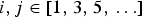 $i,j \in [1,{\kern 1pt} 3,{\kern 1pt} 5,\, \ldots ]$
with amplitudes A
i
A
j
.
$i,j \in [1,{\kern 1pt} 3,{\kern 1pt} 5,\, \ldots ]$
with amplitudes A
i
A
j
.
A) Analytical FMCW
In a FMCW radar, the phase and frequency takes the form
 $$\phi _{{\rm FMCW}} (t) = 2\pi \left( {f_l t + \displaystyle{{f_o - f_l} \over {2T_m}} t^2} \right)$$
 $$\eqalign{f_{{\rm FMCW}} (t) & = f_l + \displaystyle{{f_o - f_l} \over {T_m}} t, \cr & \equiv f_l + \alpha t,} $$
where the frequency goes from f l to f o in T m seconds, and α is the chirp rate. For a single return at the two-way travel time τ k , the mixer product becomes
 $$M_{\tau _k} (t) = A_X \cos (\phi _X (t))A_Y \cos (\phi _X (t - \tau _k )),$$
leading to the sum and difference frequencies
 $$\eqalign{f_{11}^ + &= \displaystyle{1 \over {2\pi}} \displaystyle{\partial \over {\partial t}}(\phi _X (t) + \phi _X (t - \tau _k )) \cr &= (f_l + \alpha t) + (f_l + \alpha (t - \tau _k )) \cr &= 2(f_l + \alpha t) - \alpha \tau _k,} $$
 $$\eqalign{f_{11}^ - & = \displaystyle{1 \over {2\pi}} \displaystyle{\partial \over {\partial t}}(\phi _X (t) - \phi _X (t - \tau _k )) \cr & = \alpha \tau _k,} $$
the beat sum,
 $f_{11}^ + $
, can be filtered out as long as 2(f
l
+ αt) ≫ ατ
k
, which is normally assured by having a slow sweep time T
m
, leaving us with the desired beat frequency ατ
k
, which is easily identified by a Fourier transform.
$f_{11}^ + $
, can be filtered out as long as 2(f
l
+ αt) ≫ ατ
k
, which is normally assured by having a slow sweep time T
m
, leaving us with the desired beat frequency ατ
k
, which is easily identified by a Fourier transform.
In a square wave FMCW radar, the mixer will, as seen in (1), not only mix the fundamental frequency terms, but also mix the harmonics. Writing out (2) when we include the third harmonic, we obtain
 $$ \eqalign{& {f_{11}^ - = \alpha \tau _k \quad f_{11}^ + = 2\alpha t - \alpha \tau _k + 2f_l}, \cr & {f_{33}^ - = 3\alpha \tau _k \quad f_{33}^ + = 6\alpha t - 3\alpha \tau _k + 6f_l,} \cr & {f_{13}^ - = - 2\alpha t + 3\alpha \tau _k - 2f_l \quad f_{13}^ + = 4\alpha t - 3\alpha \tau _k + 4f_l,} \cr & {f_{31}^ - = 2\alpha t + \alpha \tau _k + 2f_l \quad f_{31}^ + = 4\alpha t - \alpha \tau _k + 4f_l.}} $$
Even when including higher order harmonics, the resulting frequencies are, as seen above, linear in time t. The third harmonic from each input mixes together and creates multiples of the beat difference (and beat sum)
 $f_{33}^ \pm = 3f_{11}^ \pm $
, while the cross-terms result in various integer slopes.
$f_{33}^ \pm = 3f_{11}^ \pm $
, while the cross-terms result in various integer slopes.
These slopes can be seen in the left column of Fig. 2, where we have plotted the entire mixer output spectogram as the first row, a zoomed view in the middle row and a Fourier transform of the beat spectrum in the bottom row. In addition, we have included the effect of a sampled transmitter, where the down-aliasing is visible as a folding around half the transmitters clock rate.

Fig. 2. Analytical, simulated, and measured beat spectrum for a square wave FMCW sweep from 38.1 to 799 MHz in 25.3 µs. Top: spectogram of the entire mixer spectrum; middle row: spectogram of the mixer difference (beat spectrum), with a (Hanning windowed) fast Fourier transform (FFT) at the bottom. From left to right: analytical model, python simulation, and measured results on the right. The transmitter is “clocked” at 1/97 ps = 10.4 GHz; hence, the visible aliasing around 5.2 GHz. The measurements are here only the transmitter, where the mixing and delay is done entirely in software. The beat spectrum is linearized with the technique presented in Section VII.
The depicted analytical model use terms up to the 30th harmonic, where we only draw up to the 9th in the spectogram view. The spectogram views use the polynomials in (7) but aliased above the transmitters Nyquist frequency of 5.2 GHz. To create the Fourier view, the analytical model first sums up the phase terms
 $$\eqalign{y_{analytical} [nT] &= \sum\limits_{i \in [1,{\kern 1pt} 3,{\kern 1pt} 5,{\kern 1pt} \ldots ]} A_i \left[ {\sum\limits_{\,j \in [1,{\kern 1pt} 3,{\kern 1pt} 5,{\kern 1pt} 7]} A_j \cos (\phi _{ij}^ \pm [nT])} \right], \cr \phi _{ij}^ \pm [nT] &= i\phi _{{\rm FMCW}} [nT] \pm j\phi _{{\rm FMCW}} [nT - \tau _i ],} $$
where ϕ
FMCW is found in equation (3),
 $T = 97{\kern 1pt} {\rm ps}$
,
$T = 97{\kern 1pt} {\rm ps}$
,
 $T_m = 25.3{\kern 1pt} {\kern 1pt} {\rm \mu s}$
, and
$T_m = 25.3{\kern 1pt} {\kern 1pt} {\rm \mu s}$
, and
 $n \in [0,\,{\kern 1pt} 1,{\kern 1pt} \ldots, {\kern 1pt} T_m /T]$
. The waveform is then upsampled and zero padded before a Hanning windowed Fourier transform.
$n \in [0,\,{\kern 1pt} 1,{\kern 1pt} \ldots, {\kern 1pt} T_m /T]$
. The waveform is then upsampled and zero padded before a Hanning windowed Fourier transform.
A square wave mixer has a large number of intermixing products. In addition to handle harmonics, care must be taken when selecting the sweep parameters f l , f o , and T m to minimize the interference of the mixer cross-terms. As the mixer cross-terms are not constant in time, their interference does not cause false targets, but rather raises the noise floor.
B) Analytical CW/SFCW
Transmitting a single frequency f c , a square wave mixer sees the inputs
 $$\phi _X = 2\pi f_c t,$$
 $$\phi _Y = 2\pi f_c (t - \tau _k ).$$
We notice that a frequency domain investigation is insufficient, as we simply get
 $$f_{ii}^ - = f_{jj}^ - = 0\quad {\rm for}\;i,j \in [1,\,3,\,5,\, \ldots ],$$
i.e. the fundamental and all of the harmonic differences will mix down to DC. Looking instead at the phase, we obtain
 $$\eqalign{& {\phi _{11}^ - = 2\pi f_c \tau _k \quad \phi _{11}^ + = 2\pi f_c (2t - \tau _k ),} \hfill \cr & {\phi _{33}^ - = 6\pi f_c \tau _k \quad \phi _{33}^ + = 6\pi f_c (2t - \tau _k ),} \hfill \cr & {\phi _{13}^ - = 2\pi f_c ( - 2t + 3\tau _k )\quad \phi _{13}^ + = 2\pi f_c (4t - 3\tau _k ),} \hfill \cr & {\phi _{31}^ - = 2\pi f_c (2t + \tau _k )\quad \phi _{31}^ + = 2\pi f_c (4t - \tau _k ).} \hfill } $$
The “classical” result is here the phase
 $\phi _{11}^ - $
, which gives a (ambiguous) range estimate at
$\phi _{11}^ - $
, which gives a (ambiguous) range estimate at
 $$\phi _{11}^ - = 2\pi (f_c \tau _k + n)\quad {\rm for}\;n \in \pm [0,\,1,\,2,\,3, \ldots ],$$
which can be solved for the two-way travel time of target k
 $$\tau _k = \displaystyle{{\phi _{11}^ -} \over {2\pi f_c}} - \displaystyle{n \over {f_c}}, $$
we notice that the ambiguity of phase wrapping creates false targets every 1/f c . To improve this, we need to measure with multiple frequencies f c , say N frequencies spaced Δf c apart, each frequency being transmitted for Δt c seconds. We now have a SFCW radar, where the change in measured phase gives the range information [Reference Nguyen and Park16]
 $$f_{{\rm SFCW}} = \displaystyle{1 \over {2\pi}} \displaystyle{{\partial \phi _{11}^ - (f_c )} \over {\partial t}},$$
 $$= \displaystyle{\partial \over {\partial t}}\left( {f_c \tau _k a + n} \right),$$
 $$= \tau _k \displaystyle{\partial \over {\partial t}}f_c, $$
which is just the discrete equation
 $$= \tau _k \displaystyle{{\Delta f_c} \over {\Delta t_c}}. $$
In a similar manner to the FMCW radar, we now have a direct link between a frequency and the two-way travel time of the target. This is however inherently sampled, following [Reference Nguyen and Park16], the ambiguity of Δf c discrete frequency steps creates aliasing around τ = 1/(2Δf c ). A tight number of steps is therefore required to avoid far off returns appearing as aliased responses.
There is no strict requirement for I/Q sampling, as the phase at each step
 $\phi _{11}^ - (f_c )$
is never explicitly needed in the processing, we simply use the real-valued samples for each SFCW step to recreate the environments transfer function. We therefore achieve the same final result as an I/Q SFCW radar by sampling with twice the number of frequencies. From (10) we notice that the output of interest lies at DC, so for each SFCW step, we simply store the mean mixer output value. The f
SFCW is then found to be a Fourier transform, alternatively, we can get τ
k
directly from an inverse Fourier transform.
$\phi _{11}^ - (f_c )$
is never explicitly needed in the processing, we simply use the real-valued samples for each SFCW step to recreate the environments transfer function. We therefore achieve the same final result as an I/Q SFCW radar by sampling with twice the number of frequencies. From (10) we notice that the output of interest lies at DC, so for each SFCW step, we simply store the mean mixer output value. The f
SFCW is then found to be a Fourier transform, alternatively, we can get τ
k
directly from an inverse Fourier transform.
The aliasing does however represents a challenge for a square wave SFCW radar. In the FMCW case, the ambiguous/additional responses at iατ
k
(for
 $i \in [3,{\kern 1pt} \,5,\, \ldots ]$
) can be filtered by an anti-aliasing filter before sampling the beat frequency. In the SFCW case, the undesired phase terms i2πf
c
τ
k
will create the sampled frequencies iτ
k
Δf
c
/Δt
c
, which will fold into signal band if left unmanaged.
$i \in [3,{\kern 1pt} \,5,\, \ldots ]$
) can be filtered by an anti-aliasing filter before sampling the beat frequency. In the SFCW case, the undesired phase terms i2πf
c
τ
k
will create the sampled frequencies iτ
k
Δf
c
/Δt
c
, which will fold into signal band if left unmanaged.
The solution is identical to a superheterodyne receiver, where instead of using a single frequency, we transmit one frequency and mix with a frequency that is offset by f c + f offset . The mixer difference will produce the offset frequency, and the harmonics mix to create [3f offset , 5f offset , …], which can be filtered out.
We will return to a square wave SFCW radar in Section IV, but first, we must deal with the harmonics.
III. DEALING WITH HARMONICS
As we have seen, a frequency-modulated radar will, after a Fourier transform, have ambiguous returns at integer multiples of the true target. Although these ambiguous returns are lower in amplitude, they will appear indistinguishable from weaker true targets. A method to circumvent the ambiguity was first presented in [Reference Bjørndal, Hamran and Lande17], where we briefly presented how a delay on the receiver separated the harmonics from the signals. This was then extended in [Reference Bjørndal, Hamran and Lande14], where we not only showed how to move the targets out of band, but also how to utilize the harmonics constructively and an alternative technique that suppresses the harmonics in-band. In this paper, we have refined the simulation setup and the correlation technique.
The advantage of using a bitstream as the waveform is that implementing a programable time delay is realistic. This enables an array of new radar signal processing opportunities, since we can now freely adjust the range response, making targets appear closer or further away depending on which path is delayed. In a square wave frequency-modulated radar, this functionality is useful, since it gives multiple methods to separate the harmonics from the fundamental.
There are multiple ways to implement the programable delay. In continuous time, we can use a series of digitally selectable inverters. In a synchronous implementation, we can duplicate the generator and program in a time-offset between them. One generator then feeds the mixer, while the other is used for transmission. A delay inserted in the on-chip path between the generator and mixer will decrease the apparent two-way travel time of the response, while a delay in the channel path will make the environment response appear further away. For the channel path, which is the programable delay we will use here, the delay can either be inserted on the receiver (after the threshold, as depicted in [Reference Bjørndal, Hamran and Lande17]) or, equivalently, on the transmitter; as both placements increase the apparent two-way travel time. We will denote this adjustable delay as τ tx .
A) Moving out of band
The first method we will present requires a delay equal to (or greater) than the desired unambiguous range r un . A delay of τ tx = τ un = 2r un /c will move the fundamental of the direct return to ατ un with its second harmonic now moved to 2ατ un . This creates a unambiguous band for the fundamental, allowing us to ignore (filter away) the harmonics.
To illustrate this technique, we simulate a square wave FMCW radar (as indicated in Fig. 1) and obtain the beat spectrums in Fig. 3. For simplicity, we here view everything as continuous time and care is taken in the simulation to minimize aliasing when modeling the square waves in a discrete simulation. We do not include the typical low-pass filtering and sampling of the beat spectrum.

Fig. 3. Simulated scenario to illustrate how a delay in the channel path can separate the fundamental from the harmonics. A square wave chirp, where the fundamental goes from 600 MHz to 2.67 GHz in
 $16.7{\kern 1pt} {\kern 1pt} {\rm \mu s}$
is repeated 20 times with a linearly varying thresholds for each chirp. The first panel uses no delay and shows five equal amplitude targets interwoven with harmonics. By increasing the delay, by
$16.7{\kern 1pt} {\kern 1pt} {\rm \mu s}$
is repeated 20 times with a linearly varying thresholds for each chirp. The first panel uses no delay and shows five equal amplitude targets interwoven with harmonics. By increasing the delay, by
 $2 \cdot 100{\kern 1pt} {\rm m}/c = 667{\kern 1pt} {\rm ns}$
, the next panel (middle) shows the harmonics moved out of the highlighted fundamental band. At the bottom, we increase the delay even further to separate the third and fifth harmonic, allowing us to utilize the higher resolution of the third harmonics. Originally proposed in [Reference Bjørndal, Hamran and Lande14].
$2 \cdot 100{\kern 1pt} {\rm m}/c = 667{\kern 1pt} {\rm ns}$
, the next panel (middle) shows the harmonics moved out of the highlighted fundamental band. At the bottom, we increase the delay even further to separate the third and fifth harmonic, allowing us to utilize the higher resolution of the third harmonics. Originally proposed in [Reference Bjørndal, Hamran and Lande14].
In Fig. 3, we simulate five targets distributed between 0 m and
 $r_{un} = 100{\kern 1pt} {\rm m}$
using increasing delay settings in the channel path. Without delay, the close in targets will have harmonics interwoven with targets further out. As we increase the delay, we can not only get an unambiguous frequency range for the fundamental (middle panel), but we can also get an unambiguous range for the individual harmonics.
$r_{un} = 100{\kern 1pt} {\rm m}$
using increasing delay settings in the channel path. Without delay, the close in targets will have harmonics interwoven with targets further out. As we increase the delay, we can not only get an unambiguous frequency range for the fundamental (middle panel), but we can also get an unambiguous range for the individual harmonics.
Remember that the third harmonic components are created by the mixing the third harmonics of the two mixer inputs; this means that a sweep with bandwidth BW = f o − f l has third harmonics sweeping 3f o − 3f l = 3BW. This gives us three times the bandwidth, and hence three times the resolution! We show this resolution in the bottom panel of Fig. 3, where two targets separated by 136 mm are barely separated when we use the fundamental, but is clearly separated when looking at the third harmonic in the beat spectrum.
The only requirements for utilizing the harmonics is that (a) the mixer is digital and (b) that we can look at the harmonics without ambiguity. We will show the first requirement in Section VII.B, where we simulate a digital XOR gate with sinusoidal inputs, but we will first show a second way of getting an unambiguous spectrum.
B) Resolving in band ambiguity
If the desired unambiguous range is large, the above approach may necessitate an impractically long delay. As an alternative approach, we have therefore proposed a second solution. The idea is that instead of moving the harmonics all the way out of the band, we can make repeated measurements with different delays, in essence giving us staggering or jittering in the beat spectrum. If we do a frequency shift of the spectrum, both the fundamental and harmonics will shift by the same frequency, while a delay will cause the fundamental to shift by a different amount than the harmonics. Assuming the non-delayed response is
 $$F = [f_i, \,3f_i, \,5f_i, {\kern 1pt} \, \ldots ]$$
a new measurement with a delay τ tx on the receiver results in
 $$F_{\tau _{tx}} = [f_i + \alpha \tau _{tx}, \,{\kern 1pt} 3(f_i + \alpha \tau _{{\rm tx}} ),\,5(f_i + \alpha \tau _{{\rm tx}} ),{\kern 1pt} \, \ldots ].$$
Shifting this back by f shift = ατ tx results in
 $$\eqalign{F_{f_{shift}} &= F_{\tau _{tx}} - f_{shift} \cr &= [f_i, \,3(f_i + \alpha ) - \alpha \tau _{tx}, \,5(f_i + \alpha \tau _{tx} ) - \alpha \tau _{tx}, \, \ldots ].} $$
We notice that the fundamentals of F and
 $F_{f_{shift}} $
lines up at f
i
, while the harmonics do not. The shift is simplest to achieve after a Fourier transform, as a re-arrangement of indices.
$F_{f_{shift}} $
lines up at f
i
, while the harmonics do not. The shift is simplest to achieve after a Fourier transform, as a re-arrangement of indices.
By measuring with different delay settings of τ tx and compensating for the expected shift, the range profiles can be averaged. This effectively dithers away the undesired harmonic responses, while improving the SNR.
As an alternative to averaging, we can in some cases, reduce clutter level with fewer measurements by correlating the shifted and delayed spectrum. To maintain the voltage unit, the correlation is calculated as
 $$X_{corr} = \sqrt {\left \vert {X_{f_{shift}} X_{\tau _{tx}}} \right \vert}. $$
Where, without the square root, voltage units would be transformed to power units.
An example simulation is shown in Fig. 4. As in Section III.A, each sweep covers a bandwidth of 2.67 GHz–600 MHz = 2 GHz in
 $16.7{\kern 1pt} {\rm \mu s}$
, but is here repeated 128 times to detect the weaker return placed 40 dB below the two stronger returns. In addition, additive white Gaussian noise (AWGN) is added to the channel, with the same rms amplitude as the signal (giving an input SNR of 0 dB). The time bandwidth product of the chirp and the coherent averaging of the sweep threshold receiver gives a theoretical SNR improvement of
$16.7{\kern 1pt} {\rm \mu s}$
, but is here repeated 128 times to detect the weaker return placed 40 dB below the two stronger returns. In addition, additive white Gaussian noise (AWGN) is added to the channel, with the same rms amplitude as the signal (giving an input SNR of 0 dB). The time bandwidth product of the chirp and the coherent averaging of the sweep threshold receiver gives a theoretical SNR improvement of
 $2\,{\kern 1pt} {\rm GHz} \times 16.7\,{\rm \mu s} \times 128 = 66\,{\rm dB}$
, which is consistent with the here simulated SNR of 70 dB.
$2\,{\kern 1pt} {\rm GHz} \times 16.7\,{\rm \mu s} \times 128 = 66\,{\rm dB}$
, which is consistent with the here simulated SNR of 70 dB.

Fig. 4. Simulated scenario to illustrate the correlation technique to suppress harmonics in-band. Three targets are simulated, two closely spaced targets and one weaker return. AWGN noise is added to the channel with the same rms amplitude as the signal (input SNR of 0 dB). The top panel shows a sweep where the radar is programed without any delay. In the next panel, the sweep is repeated with a delay of
 $\tau _{tx} = 42{\kern 1pt} {\rm ns}$
in the channel path; this is then shifted back by
$\tau _{tx} = 42{\kern 1pt} {\rm ns}$
in the channel path; this is then shifted back by
 $f_{shift} = \alpha \tau _{tx} = 5.2{\kern 1pt} \;{\rm MHz}$
. The bottom panel shows the point wise multiplication (correlation) of the original and shifted spectra. Similar to [Reference Bjørndal, Hamran and Lande14].
$f_{shift} = \alpha \tau _{tx} = 5.2{\kern 1pt} \;{\rm MHz}$
. The bottom panel shows the point wise multiplication (correlation) of the original and shifted spectra. Similar to [Reference Bjørndal, Hamran and Lande14].
We see in Fig. 4 that the fundamentals line up while the harmonics are reduced (limited by the noise floor). It is clear that the weak signal is ambiguous with the harmonics of the stronger scatters, without the correlation. In this example, we line up the fundamental, but the technique can also be used to line up the harmonics, giving the same improved resolution as was demonstrated in the previous section.
The correlation technique relies on the harmonics lining up with “empty” parts of the range spectrum and is therefore best suited for “sparse” scenes with few returns, or at least scenes with some empty regions. The two presented techniques can be combined to alleviate this, by moving at least some of the harmonics up and correlating or averaging away the rest. An optimal choice of delay settings and harmonic suppression technique will depend on the image scene, which, due to the ease of digital integration, can conceivably be optimized automatically.
IV. SFCW
As was explained in the analytical section (Section II.B), a SFCW radar is implemented as a CW radar that steps the output frequency. The proposed architecture to achive this is shown in Fig. 5, consisting of a CW transmitter and receiver with some control logic.

Fig. 5. Principle of a bitstream CW radar controlled by a SFCW processor. For each frequency f n , the CW radar outputs the mean (DC) value, which is arranged and transformed with an inverse fast Fourier transform (IFFT) yielding the range spectrum.
Traditionally, a CW receiver low-pass filters the mixer output and digitizes the remaining DC value with a high-resolution ADC. To avoid this analog voltage level, and the filter, we can make the observation that the mixer output will toggle like a pulse-density modulation signal. The desired DC level can then be found by measuring (counting) the ratio of high-to-low values. This is trivial to implement as two counters, one that increments if the signal is high and another that increments when the signal is low. The sampling clock does not need to be synchronous, we are simply interested in the average value, so a local free running ring oscillator can serve as the clock source.
An example simulation is shown in Fig. 6, where we step the CW frequency 1381 times from 600 MHz with a 1.5 MHz frequency step. A number of cases is illustrated; as a reference, an idealized sinusoidal simulation is shown in the top panel, giving a single peak for each simulated target. The next panel shows what happens if we do not deal with the harmonics; due to the sampled nature of a SFCW radar, the harmonics will fold around
 $1/(2 \cdot 1.5{\kern 1pt} \;{\rm MHz}) = 334{\kern 1pt} \;{\rm ns}$
. By taking this folding into account, we can annotate the peaks by using the fundamental peak as a reference, peaks up to the 19th harmonic is visually recognizable.
$1/(2 \cdot 1.5{\kern 1pt} \;{\rm MHz}) = 334{\kern 1pt} \;{\rm ns}$
. By taking this folding into account, we can annotate the peaks by using the fundamental peak as a reference, peaks up to the 19th harmonic is visually recognizable.

Fig. 6. Simulated SFCW radar with two close targets, the radar is stepped from 600 MHz to 2.67 GHz in 1381 steps of length 53 µs (divided into 16 different threshold settings). The top panel shows an idealized (sinusoidal) simulation, with an inset showing the two simulated targets separated by 121 mm and the −31 dB sidelobe level of the Hanning window barely visible. In the next panel, a square wave SFCW radar is simulated and harmonic peaks up to the 19th harmonic are annotated. The harmonics are attenuated by adding a frequency offset of 30 kHz between the two mixer inputs and using averaging as a simple to implement filter. In the bottom panel, we do not use a frequency offset, but simulate the transmitter with a finite time resolution of 64 ps, jitter levels measured in [Reference Bjørndal, Hamran and Lande17] and an input SNR of 0 dB. This effectivly dithers away the higher order harmonic peaks.
As was mentioned in the analytical section, the theoretical solution is to add a frequency offset between the transmitted and mixed signal, the low-pass characteristic of taking the average then attenuates the higher order harmonics as shown in the next panel. An alternative to attenuating the harmonics is to jitter them away; this could be added explicitly by modifying the bitstream, but we first consider some real-world deviations from a perfect square wave.
The first such non-ideal behavior is finite time resolution, the bitstream consists of discrete bits, which is read out with a finite clock rate. In addition, the transmitter will have jitter, we here include the measured jitter level from [Reference Bjørndal, Hamran and Lande17] and also added some AWGN noise to the channel. These effects create the bottom panel of Fig. 6. We note that these real-world effects jitter away the higher harmonic peaks, without requiring a frequency offset.
V. CORRELATION-BASED RADAR
We have up to now discussed radar architectures that are frequency modulated. These rely on a single mixer to down-convert the received signal and a Fourier transform of the captured data to obtain a range spectrum. A more general architecture is proposed in Fig. 7, where we have replaced the mixer with a correlation circuit. In a correlation-based radar, we can utilize any waveform, where “noise radars” (usually pseudo noise) are most common. The correlation circuit can be in continuous time, as shown by the correlating circuit in [Reference Hjortland and Lande15], or discrete.

Fig. 7. Principle of a bitstream-based radar that does a full correlation between the transmitted and received signal. The correlation circuit can either be sampled; by using a chain of D-flip-flops, or continuous time; by using inverters as delay elements.
A particularly nice set of pseudo random noise (PN) sequences are coined maximum length sequences (M-sequences) and can be generated with a single linear feedback shift register (LFSR). Sachs [Reference Sachs5] gives a thorough overview on M-sequence radar. The repetition of a pseudo random sequence gives a range ambiguity given by the sequence length, while the bandwidth (and hence the resolution) is proportional to the sequence rate.
In addition, an M-sequence has “perfect” autocorrelation, with a peak of 1 and the value − 1/N for all other delays. This gives us the dynamic range for a single target scenario. For a more realistic scenario, with multiple returns, the floor − 1/N adds up, decreasing the dynamic range for each return.
Figure 8 shows a simulated and measured M-sequence after correlation. Two sequences are compared, a shorter 29 − 1 = 511 sequence and a 212 − 1 sequence. The sequences are repeated continously and read out at a clock rate of
 $1/(2 \cdot 88.4{\kern 1pt} {\rm ps}) = 5.7{\kern 1pt} {\rm GHz}$
. The first sequence repeates after 90 ns, while the other after 724 ns.
$1/(2 \cdot 88.4{\kern 1pt} {\rm ps}) = 5.7{\kern 1pt} {\rm GHz}$
. The first sequence repeates after 90 ns, while the other after 724 ns.

Fig. 8. Simulated M-sequence radar with two close targets. The top panel uses a nine-stage LFSR, while the bottom panel uses a m = 12 stage. On the left, the entire system is simulated [Reference Bjørndal, Hamran and Lande14], on the right, the waveform generator is measured and used in the simulation. The simulation is averaged over 32 different threshold levels and include band-limited noise with σ = 0.1.
VI. UNMODULATED PULSED RADAR
The previously presented radar types can easily be used in pulsed mode (or interrupt mode), where the transmitter is occasionally turned off. Shutting down the transmitter is traditionally done to avoid saturating the receiver, long-range radars can transmit long “pulses” of a modulated waveform and then shut the transmitter off before capturing the backscattered data. The modulation can be any of the mentioned radar architectures, either frequency modulated or even a pseudo random sequence.
In this section, we will have a brief look at a simpler unmodulated radar, where no pulse compression is performed. An unmodulated radar is in principle simpler to implement; we simply transmit a single pulse and get the range response by synchronously capturing the received signal. We do however loose the advantage of a modulated waveform (either pulsed or continuous), in that the receiver takes advantage of a matched filter, presented in this paper as either a mixer or a correlator, theoretically maximizing the SNR. An additional disadvantage of pulsing the transmitter, with a limited peak output power, is the reduction in average transmitted power and hence maximum range.
In an unmodulated pulsed radar, the resolution is directly proportional to the pulse width T as
 $$\Delta R = \displaystyle{{cT} \over 2}.$$
As seen in Fig. 9, the prototype waveform generator can transmit pulses as short as 120 ps, giving us a theoretical resolution of 18 mm. The inherent flexibility of a programable bitstream allows for adjustable bandwidth as shown by the difference between the “11” and “111” waveform. To conform to regulations, we can also insert notches in the mainlobe, as seen by two example double pulses “110011” and “1110000111”.

Fig. 9. Measurements of the waveform generator as a flexible pulse generator. Top: time-domain view (different waveforms offset vertically for clarity). Bottom: frequency domain view, found by the Welch method with a Hanning window and zero padding. The shortest pulse (“11”) has a measured 50 pulse width of 120 ps and a 10 dB bandwidth of 5 GHz.
VII. MEASUREMENTS
In the preceding sections, we have included measurements of the transmitter; programed for a FMCW chirp bitstream in Fig. 2, M-sequence bitstream in Fig. 8, and pulsed in Fig. 9. The transmitter is a slightly improved version of the one published in [Reference Bjørndal, Hamran and Lande17]. The chip also features a receiver, with a thresholder from Novelda [3], a XOR gate, and the CW receiver counters depicted in Fig. 5. The prototype is realized in a low-power commercial 90 nm process. We will show the XOR gate in Section VII.B with a post-layout simulation and a FMCW measurement utilizing the generator, thresholder, and mixer in Section VII.C.
The chip is programed using a Raspberry Pi communication over Serial Peripheral Interface Bus (SPI) and the threshold is set using an external digital-to-analog converter. The CW counters can be accessed with the SPI interface, so with a SPI capable device we can realize a standalone SFCW radar. The chip can be used as a FMCW radar by externally sampling the XOR output as depicted in Fig. 10 and doing a FFT on the captured data.

Fig. 10. Test setup when measuring the entire system. The chip is configured via SPI to the desired bitstream, it then transmits once the digital RUN signal enables. The channel is here emulated by a long coax. After going though the coax, the signal is compared with the externally set threshold current (I TH ) before being mixed and sent out of the chip again. The intermediate frequency (IF) is then sampled by an oscilloscope, which has an amplifier in front, to reduce noise. The chip is mounted in a standard QFN48 package (pictured with the lid of) and all of the surface-mount device (SMD) components are decoupling capacitors. Note that there is no external clock/frequency reference as the chip is self-timed.
The waveform generator is programed by writing the bitstream waveform to a 32 kb on-chip-memory. Under typical supply and bias settings (supply and N-well at 1.2 V), the chip will read out this bitstream once every 16.7 µs. This can be slowed down by increasing the N-well voltage or decreasing the supply voltage to the transmitter.
A) FMCW linearity correction
Due to the transmitter being open loop, the transmitted chirp does not linearly increase in frequency. We correct for this using the efficient technique presented in [Reference Scheiblhofer, Schuster and Stelzer18]. The linearization re-samples the beat spectrum and corrects for first-order non-linearity in the chirp, the idea starts by equating the measured beat with a constant frequency sine wave
 $$2\pi f_{beat} \cdot t_{old} [n] = 2\pi f_{meas} [n] \cdot t_{new} [n],$$
where f beat = α 1 τ is a constant. If we assume the measurements to follow
 $$f_{meas} [n] = \tau (\alpha _1 + \alpha _2 t_{new} [n]),$$
where α 2 is the unwanted first-order non-linearity term, we can solve (18) to obtain our new sampling locations
 $$t_{new} [n] = - \alpha _{12} \pm \sqrt {\alpha _{12}^2 + 2\alpha _{12} t_{old} [n]}, $$
 $${\rm where}\quad \alpha _{12} \equiv \displaystyle{{\alpha _1} \over {2\alpha _2}}. $$
Possibly due to a software bug, we have found the above equation to give complex time locations; removing a factor of 2 has empirically given better results:
 $$t_{new} [n] = - \alpha _{12} \pm \sqrt {\alpha _{12}^2 + \alpha _{12} t_{old} [n]}. $$
The α 1 and α 2 are extracted from the beat spectrum by fitting a second-order polynomial through the extracted phase. The phase is extracted by a Hilbert transform of the beat spectrum when there is only one target.
B) XOR gate as a digital mixer
We have stated that the only requirement for the harmonics to exist in a frequency-modulated radar is that the mixer is digital. This implies that attenuation of the transmitter harmonics have little consequence to the presented principles; in addition, the digital mixer can even be used in a traditional analog radar. To show this, we present a post-layout simulation from a commercial low-power 90 nm CMOS process, where the inputs are sinusoidal.
A static and symmetric XOR gate is realized with four symmetric NAND gates [Reference Weste and Harris19]; a layout is created and the parasitics are extracted. For realistic drive and load conditions, buffers are added to the XOR input and output as shown in Fig. 11. In addition, a simple model for the supply pads is included in the circuit model, consisting of a 50 fF capacitor and a 2 nH inductor.

Fig. 11. Post-layout simulation setup and results for a chirped sinusoidal input A(t), and a delayed sinusoidal responce from two targets B(t) = A(t − τ 1)/2 + A(t − τ 2)/2. The insets of the two top panels show the sinusoidal inputs in time, where the dashed curve is the sinusoidal input and the whole black line is after the four inverters. Bottom plot shows a zoomed spectogram of the buffered XOR output, where the inset includes a low-pass filtered responce as a visual reference [Reference Bjørndal, Hamran and Lande14].
As seen in Fig. 11, the buffers have more than sufficient gain to drive the output to saturation, giving us a square wave digital signal with harmonics. These harmonics will mix, creating additional peaks in the beat spectrum at multiples of the expected beat frequency. We note that a perfect 50% high/low waveform only has odd harmonics, while even harmonics are seen in the simulated XOR output.
C) Full system measurements
To show the full system, we connect the chip as shown in Fig. 10 and produce Fig. 12. The transmitter is here programed for a shorter sweep, only 418 ns long. The XOR output (IF) is captured by a oscilloscope, and the result is coherently averaged and Fourier transformed on a computer. The transmitter is connected to the receiver through a 43 ns long coax; the resulting beat frequency peak at 51 MHz corresponds to a two-way travel time of 42 ns. The reader should note that the post-layout simulation uses the extracted measured delay in the simulation; hence, the match between simulated and measured peak beat frequency comes as no surprise.

Fig. 12. Post-layout simulation (left) and measurements (right) of a digital XOR gate mixing bitstreams. The measurements are for the full system, the waveform generator is transmitting a bitstream chirp from 1 to 1.5 GHz in 418 ns and clocked out at 15.7 GHz though a 43 ns long coax, the return is then quantized and mixed with the transmitted copy before being sent out of the chip, amplified, and captured by an oscilloscope. The post-layout result is from a single simulation, while the measurements are the result of coherently averaging 283 times with different threshold levels.
VIII. DISCUSSION
Previous all digital designs like those outlined in [Reference Staszewski20, Reference Pozsgay, Zounes, Hossain, Boulemnakher, Knopik and Grange21] focus on digitally assisting the generation and capture of analog waveforms. The novelty in this work is that the waveform itself is a digital bitstream, allowing for digital generation and processing with simple digital gates.
The implementation chosen in this work is digital, asynchronous, and (mostly) continuous time.Footnote 1 Concepts presented in this paper are however fully compatible with a synchronous digital implementation, or even traditional analog. Of particular note is the increase in resolution when mixing the harmonics, as have been shown, the harmonics can be taken advantage of without a full digital implementation. The transmitting and receiving antennas and amplifiers do not need to support the larger bandwidth of the harmonics. The drawback is that the fundamental and harmonics must be separated and that the various mixer cross-terms will lower the dynamic range.
A digital asynchronous implementation has the advantage of pushing modern technology to its limits, as it can take full advantage of the fine time delay of digital gates without the added overhead of timing margins and fast clock distribution. The achieved equivalent clock rate of 15.7 GHz would not be possible using standard synchronous design as a standard cell flip flop has a maximum clock rate below 8 GHz in the utilized 90 nm process.Footnote 2 Clock margins is avoided by “self-timed” chip design, enabling speed tuning using supply rails. This enables an open-loop transmitter, where the output frequency will depend on voltage and temperature, making precise and stable frequency generation under voltage and temperature variations impossible without some form of feedback. For the frequency-modulated architecture, feedback can be added by using a phase-locked loop with a stable frequency reference and an adjustable oscillator and divider, at the cost of significantly reduced flexibility as one is now limited to frequency-modulated waveforms within the oscillator's frequency range. Alternatively the waveform generator can use a fast and stable clock to read out the bitstream, at the cost of significantly lower sample rate and an increase in power consumption.
Programing the bitstream waveform by storing the bit stream in memory gives maximum flexibility and is ideal for our prototype. That said, dedicated on-chip generators for the trivial M-sequence bitstream or even a direct digital synthesizer like frequency and phase counter would most likely be far more area and power efficient for these dedicated architectures.
In a conventional FMCW radar, the chirp rate is kept low (typically on the order of 100 MHz/1 ms = 1 × 10¹¹ Hz/s); this reduces the sample rate of the beat spectrum. In our work, the single-bit beat spectrum is easier to sample at high speeds, and the waveform memory imposes a maximum limit on our chirp length; in addition, the lack of a frequency lock means we can easily transmit chirp rates on the order of 2 GHz/20 μs = 1 × 10¹⁴ Hz/s. Our high chirp rate allows the chirp to be repeated 50 times and still get a frame rate similar to a conventional radar, easing our assumption of a stationary scene.
This high chirp rate and low center frequency also allows us to safely ignore Doppler shift. For a target moving at the speed of sound
 $v_r = c_{sound} = 340{\kern 1pt} {\rm m}/{\rm s}$
and a chirp time of
$v_r = c_{sound} = 340{\kern 1pt} {\rm m}/{\rm s}$
and a chirp time of
 $T_m = 17{\kern 1pt} {\rm \mu s}$
around
$T_m = 17{\kern 1pt} {\rm \mu s}$
around
 $f_c = 1{\kern 1pt} \;{\rm GHz}$
, we expect a Doppler shift of only around
$f_c = 1{\kern 1pt} \;{\rm GHz}$
, we expect a Doppler shift of only around
 $2v_r f_c /c = 2.3{\kern 1pt} \;{\rm kHz}$
, which is in essence a DC signal considering our chirp time and the assumed (fast!) speed.
$2v_r f_c /c = 2.3{\kern 1pt} \;{\rm kHz}$
, which is in essence a DC signal considering our chirp time and the assumed (fast!) speed.
Further study is required before the proposed principles can be applied to complex scenes with multiple moving targets (both with and without Doppler shift). One workaround is to apply multiple single-bit parallel receivers, which is very feasible since the single-bit processing is so area efficient. A multi comparator receiver will reduce the integration time in low noise scenarios and hence further ease the assumption of a stationary scene during the measurement period.
IX. CONCLUSION
We have shown the feasibility of implementing several classical frequency-modulated architectures, a pseudo noise correlation radar and a simple pulsed radar; all in single-bit CMOS implementation. Using bitstreams enables mixer operation of a frequency-modulated radar to be implemented as a single CMOS XOR gate, which is proven by analytical treatment, post-layout simulations, and measurements. The digital nature of the radar also allows such operations as delays, which are proven useful to deal with the ambiguity created by harmonics as well as increasing the theoretical resolution by a factor of 3. Preliminary measurements from a digital asynchronous implementation in CMOS prove the feasibility of bitstreams for generic single-chip radar.
 Øystein Bjørndal was born in 1989 and received his Master degree in Electronics and Computer Technology from the University of Oslo, Norway, in 2013. Currently he is finishing his Ph.D. degree at the Norwegian Defence Research Establishment in cooperation with the Nanoelectronics Group at the University of Oslo; with the title “Single Bit Radar Systems for Digital Integration”. His research interests include asynchronous digital design and digital RF for radar applications.
 Svein-Erik Hamran received an M.Sc. in Technical Physics in 1984 from Norwegian University of Science and Technology (NTNU, Trondheim, Norway) and a Ph.D. degree in 1990 in Physics from the University of Tromsø. He worked from 1985 to 1996 at the Environmental Surveillance Technology Programme and was in 1989/90 a Visiting Scientist at CNRS Service d'Aeronomie, Paris, France. From 1996, he has been at the Norwegian Defence Research Establishment working as a Chief Scientist managing radar programs. From 2001 to 2011, he was an Adjunct Professor in Near Surface Geophysics at the Department of Geosciences. From 2011 to 2016, he was an Adjunct Professor at the Department of Informatics, and from 2017, he is an Adjunct Professor at the Department of Technology Systems at the University of Oslo. He is the Principal Investigator of the Radar Imager for Mars’ subsurFAce eXperiment – RIMFAX on the Mars 2020 NASA rover mission and a Co-Principal Investigator on the WISDOM GPR experiment on the ESA ExoMars rover. His main interest is UWB radar design, radar imaging and modeling in medical and ground penetrating radar.
 Tor Sverre Lande is the Professor in Microelectronics, Department of Informatics, University of Oslo; and Visiting Professor, Institute of Biomedical Engineering, Imperial College, London, UK. Research interests: wideband radar/radio/RF technology, biomedical engineering, analog/mixed circuits and systems, low-power/low-voltage circuits, time-domain signal processing, wireless sensor networks, continuous-time binary-value (CTBV) processing. Co-founder of spin-off company Novelda AS (http://www.novelda.no) on wideband radar technology. IEEE Life Member, Member of IEEE BioCAS technical activities with focus on biomedical engineering. Founding Editor-in-Chief of the journal IEEE Transactions on Biomedical Circuits and Systems, Steering Committee Member of the journal IEEE Transactions on Biomedical Circuits, IEEE Fellow, IEEE CAS BoG Member, IEEE CAS Distinguished Lecturer, CAS VP Conferences and involved in a number of CAS conferences over the last two decades. TPC of ISCAS 2017. Several best paper awards. Co-author of more than 150 scientific publications. IEEE Circuits and Systems Society Meritorious Service Award, 2013. Member of Norwegian Technical Science Academy.


 Open access