1. Introduction
Earth’s most recent greenhouse to icehouse transition, from the Eocene into the Oligocene, represents one of the most significant climate changes in the Cenozoic and establishes climate trends that lasted into the Holocene Epoch. Because this transition is important for Cenozoic climate models, the Eocene–Oligocene (E–O) boundary interval, commonly called the Eocene–Oligocene transition, has been extensively studied (Katz et al. Reference Katz, Miller, Wright, Wade, Browning, Cramer and Rosenthal2008; Bohaty et al. Reference Bohaty, Zachos and Delaney2012 and references therein). The E–O boundary interval marks a critical time in recent Earth history because it coincides with the main climatic shift from relatively warm to relatively cold conditions in the Cenozoic Era (Zachos et al. Reference Zachos, Pagani, Sloan, Thomas and Billips2001, Reference Zachos, Dickens and Zeebe2008). In the southeastern United States, numerous fossiliferous localities that are temporally complete, well-exposed marine sections in riverbanks, cores and quarries allow access to fresh outcrop and fairly continuous exposures. While many studies have focused on the boundary interval and E–O transition in this region (Ellwood et al. Reference Ellwood, Mcpherson, Sen Gupta and Matthews1986; Miller et al. Reference Miller, Thompson and Kent1993, Reference Miller, Browning, Aubrey, Wade, Katz, Kulpecz and Wright2008; Dockery & Thompson, Reference Dockery and Thompson2016), inconsistencies in published work, with regard to lithostratigraphic nomenclature and the E–O boundary position, have prevented these sections from being incorporated into a global palaeoclimatic framework. The work presented here was centred on a number of localities, including five successions in the SE United States, and one, St Stephens Quarry (SSQ), was a candidate for the E–O Global Boundary Stratotype Section and Point (GSSP), the Priabonian–Rupelian stage boundary (Jovane et al. Reference Jovane, Florindo and Dinarés-Turell2004, Reference Jovane, Florindo, Sproviere and Pälike2006, Reference Jovane, Sprovieri, Florindo, Acton, Coccioni, Dall’Antonia and Dinarés-Turell2007, Reference Jovane, Coccioni, Marsili, Acton, Koeberl and Montanari2009), but ultimately, the GSSP was placed in the Massignano section located near Ancona, in central Italy (Premoli-Silva & Jenkins, Reference Premoli-Silva and Jenkins1993; Jovane et al. Reference Jovane, Coccioni, Marsili, Acton, Koeberl and Montanari2009). GSSPs are important because they provide an agreed upon standard to which other than biostratigraphic methods can be applied and therefore be used for correlation. This can aid in clarifying uncertainties in dating accuracy and precision that cloud our understanding of the timing and global synchronicity of climate change with potential forcing mechanisms. For example, it has been argued from the isotopic composition of fossilized teeth and bones of terrestrial vertebrates that the greenhouse to icehouse change occurred over ∼400 kyr (Zanazzi et al. Reference Zanazzi, Kohn, Macfadden and Terry2007). These authors, however, place the E–O boundary transition at ∼33.5 Ma, whereas others place the E–O boundary at ∼33.7 Ma (Jovane et al. Reference Jovane, Florindo and Dinarés-Turell2004, Reference Jovane, Florindo, Sproviere and Pälike2006, Reference Jovane, Sprovieri, Florindo, Acton, Coccioni, Dall’Antonia and Dinarés-Turell2007, Reference Jovane, Coccioni, Marsili, Acton, Koeberl and Montanari2009) or ∼33.9 Ma (Gradstein et al. Reference Gradstein, Ogg, Schmitz and Ogg2012; Ogg et al. Reference Ogg, Ogg and Gradstein2016), which complicates estimates for determining the total duration of the E–O cooling.
Furthermore, uncertainties in correlating marine and terrestrial ages, as well as differences in precision between various absolute dating methods, make high-resolution age estimates difficult. For these and other reasons there have been several relatively recent studies on E–O boundary exposures and cores from the SE United States that have built on the stratigraphic relationships developed over the last 150 years (e.g. Hilgard, Reference Hilgard1860; MacNeil, Reference MacNeil1944; Murray, Reference Murray1947; Toulmin, Reference Toulmin1955; Cheetham, Reference Cheetham1957; Mancini, Reference Mancini1979, Reference Mancini2000; Bybell, Reference Bybell1982; L. A. Waters (unpub. M.Sc. thesis, Univ. Alabama, 1983); Bybell & Poore, Reference Bybell and Poore1983; Coleman, Reference Coleman1983; Keller, Reference Keller1985; Mancini & Waters, Reference Mancini and Waters1986; Ellwood et al. Reference Ellwood, Mcpherson, Sen Gupta and Matthews1986; Pasley & Hazel, Reference Pasley and Hazel1990, Reference Pasley and Hazel1995; Tew & Mancini, Reference Tew and Mancini1992; Miller et al. Reference Miller, Thompson and Kent1993, Reference Miller, Browning, Aubrey, Wade, Katz, Kulpecz and Wright2008; Jaramillo & Oboh-Ikuenobe, Reference Jaramillo, Oboh-Ikuenobe, Goodman and Clarke2001; Katz et al. Reference Katz, Miller, Wright, Wade, Browning, Cramer and Rosenthal2008; Fluegeman, Reference Fluegeman, Demchuk and Gary2009; Wade et al. Reference Wade, Houben, Quaijtaal, Schouten, Rosenthal, Miller, Katz, Wright and Brinkhuis2012).
In the SE United States (Mississippi, Alabama and Florida), the E–O boundary has been identified by several authors to lie within limestone and marl units at several localities. However, because of an effort to extend and correlate ‘type’ lithologies from northwestern Mississippi through southwestern Alabama (e.g. Hilgard, Reference Hilgard1860; MacNeil, Reference MacNeil1944; Murray, Reference Murray1947, Reference Murray1952), and ultimately into the Florida Panhandle (Moore, Reference Moore1955), and from the Florida Panhandle into Alabama, unit definitions have become blurred. As a result, confusion regarding lithostratigraphic nomenclature abounds, even for the best exposures. One goal of this paper is to describe several important localities in the United States Gulf Coastal Plain and clarify lithostratigraphic nomenclature for critical exposures. Another goal is to interpret the lithologic, geochemical, geophysical and biostratigraphic datasets in the SE United States, and correlate these sections into the global stratigraphic framework using the GSSP (Premoli-Silva & Jenkins, Reference Premoli-Silva and Jenkins1993).
2. Historical setting for the Eocene and Oligocene
The development of the Geologic Column began in 1822 with the definition of the Carboniferous and Cretaceous periods (see Harland et al. Reference Harland, Armstrong, Cox, Craig, Smith and Smith1990). By 1833, the Eocene, Miocene and Pliocene epochs were defined for the Tertiary Period, but the Oligocene Epoch was not mentioned (Lyell Reference Lyell1833). Lyell (Reference Lyell1833) described Eocene fossils as being made up of 1–5% of modern marine species, and that in England, climate was warm and tropical, the first indication of a possibly global greenhouse environment during the Eocene Epoch.
It was not until ∼1854–55 that the term Oligocene (Oligocän as written in the original version by Beyrich, Reference Beyrich1856) was used by Heinrich Ernst von Beyrich, as documented by von Koenen in Reference von Koenen1867, in Geological Magazine (von Koenen, Reference von Koenen1867). The Oligocene appears not to have been accepted by most authors for several decades, given that Lyell’s Principles of Geology (Lyell, Reference Lyell1857) published in England, and Dana’s New Text-Book of Geology (Dana, Reference Dana1883) or Le Conte’s Compend of Geology (Le Conte, Reference Le Conte1884) published in the United States, include the Eocene but not the Oligocene Epoch.
Now, with the development of the modern Geologic Time Scale, the Eocene Ypresian Stage was formally ratified (defined) in 2003 (Aubry et al. Reference Aubry, Ouda, Dupris, Berggren and Van Covering2007), with an age beginning at ∼56 Ma (Ogg et al. Reference Ogg, Ogg and Gradstein2016). In turn, the beginning of the Oligocene Rupelian Stage was ratified in 1992 (Premoli-Silva & Jenkins, Reference Premoli-Silva and Jenkins1993) with an age beginning at ∼33.9 Ma (Ogg et al. Reference Ogg, Ogg and Gradstein2016).
3. Geologic setting, SE United States: sections from west to east in Figure 1
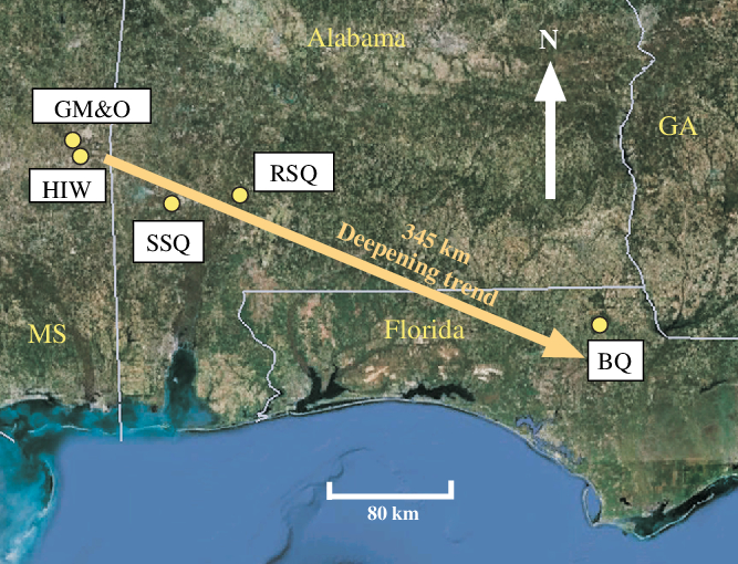
Fig. 1. Location map of E–O sections sampled from the southeastern United States (Fig. 2). GM&O – Gulf, Mobile and Ohio trestle section; HIW – Hiwannee Sections; SSQ – St Stephens Pelham Hill North Quarry composite section; RSQ – Red Stick Quarry section; BQ – Brooks Quarry section. Image modified from Google Earth. The arrow indicates a trend towards deeper marine sections, from marine clays in the northwest to marine limestone beds in the southeast. Distance represented is ∼340 km from the GM&O section in Mississippi to the BQ section in Florida.
3.a. Shubuta, Mississippi: Red Bluff Formation type section at the Gulf, Mobile and Ohio railroad trestle
Hilgard (Reference Hilgard1860) named and described the Red Bluff Formation stating it is exposed ‘on Chickasawhay River just above railroad bridge, 1.5 mi south of Shubuta, Wayne Co., MS’. We place this locality on the N-facing slope of a bluff immediately south of the Gulf, Mobile and Ohio (GM&O) railroad bridge where it crosses the Chickasawhay River, ∼2.4 km due south of the town of Shubuta, Mississippi (Fig. 1). The section, GM&O in Figure 2a, has been described as marine glauconitic clayey marl containing ferruginous streaks, hard limestone ledges and common iron concretions (Hilgard, Reference Hilgard1860; MacNeil, Reference MacNeil1944). In addition, MacNeil (Reference MacNeil1944) included beds of two lithotypes at this locality, a basal unit that is composed of limestone and glauconite-rich beds, and an upper clay member. We interpret these units as (1) the Pachuta Marl and lower part of the Shubuta Clay members of the Yazoo Formation (Fig. 2a) (Murray, Reference Murray1947), and (2) the rest of the Shubuta Clay Member where it is heavily weathered higher in the bluff. In surface exposures of this section, the glauconite has been weathered and altered to haematite, giving the bluff a red colour at the surface and leading to Hilgard’s descriptive name, Red Bluff. The limestone units here include the carbonate-rich Pachuta Marl, and a limestone lens in the Shubuta Clay Member that we refer to as the Shubuta lime bed (Fig. 2a, c). Surface alteration is generally not deep where the surface gradient is steep, and it is quite easy to clean the altered surface exposures to recover unaltered green-coloured glauconite, the primary clay in the Shubuta Clay Member. However, when the gradient in the section flattens out, weathering is deep and cleaning the section is difficult, resulting in the fact that the Red Bluff Formation, above the Shubuta Clay Member, is covered here.
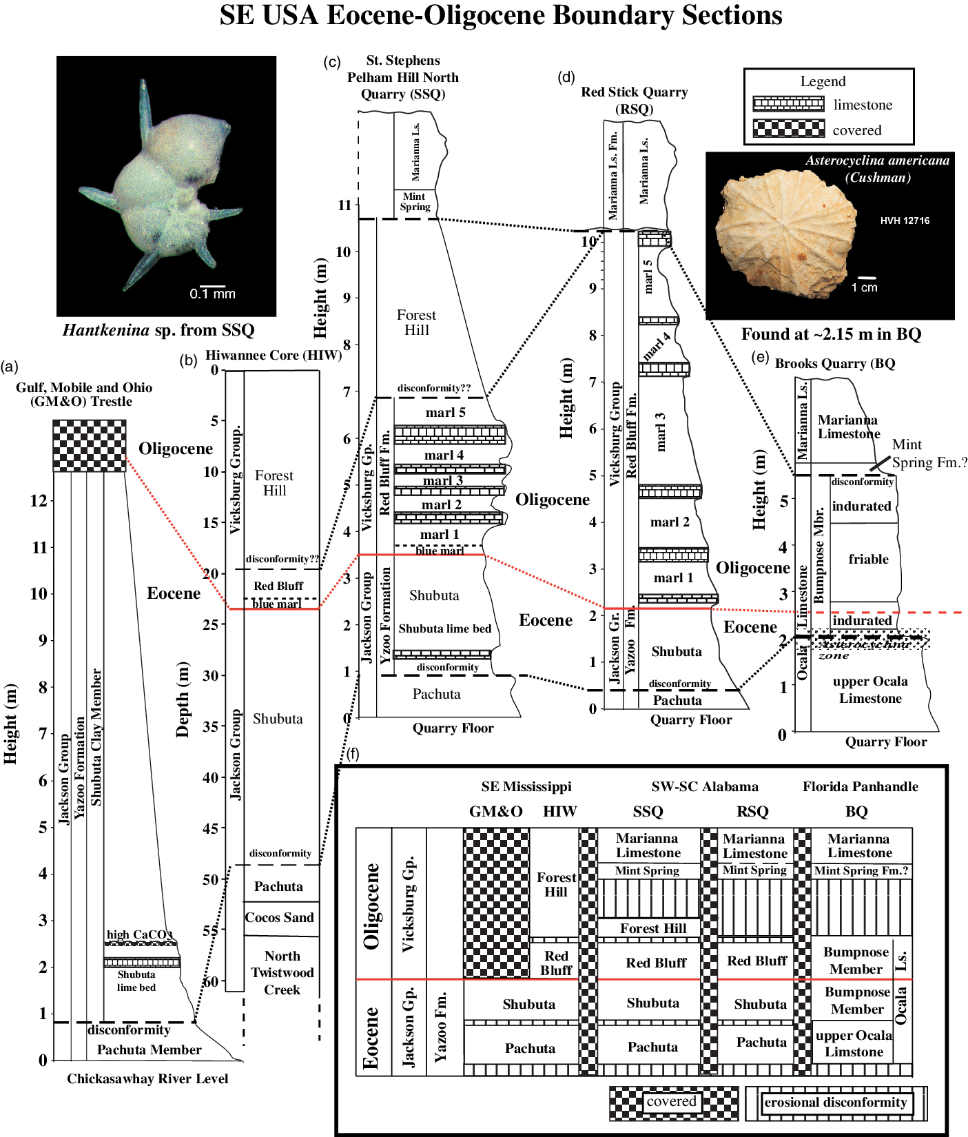
Fig. 2. Stratigraphy for sampled measured sections and the HIW core, which is directly correlated to a measured section cropping out ∼500 m to the WSW on the Chickasawhay River. Locations are given in Figure 1: (a) GM&O, (b) HIW, (c) SSQ, (d) RSQ, and (e) BQ. Solid red correlation lines represent the E–O boundary; dashed black lines represent unconformities. The E–O boundary is identified by the highest observed occurrence point (HOOP) of the Hantkeninidae family, and coincides with the transition from the Shubuta Clay Member of the Yazoo Formation, Jackson Group, into the Red Bluff Formation of the Vicksburg Group. (f) Locations as given in Figure 1, extending from SE Mississippi to the Florida Panhandle.
Approximately 1.3 km to the NNE, also on the Chickasawhay River, but where the ‘old’ US45 highway bridge crosses the river, is the type locality for the Shubuta Clay described by Murray in Reference Murray1947. At this locality, the Shubuta Clay Member is described as a clay or clayey marl that is overlain by the Red Bluff or Forest Hill Formation.
The lower part of our GM&O measured section (Fig. 2a), located on the south side of the Chickasawhay River at the GM&O trestle, is richly fossiliferous throughout, with abundant calcareous macroscopic invertebrates and microfossils, especially foraminifera. At the base of the section, beginning at river level at the time of sampling, is ∼0.8 m of a carbonate-rich, glauconitic and phosphatic marl that ends at a disconformity. In general, the marl, when freshly cleaned, has a light grey-green colour. This unit dips at ∼5° to the north, into the river. The lithologic similarity of this bed with the Pachuta Marl Member of the Yazoo Formation, defined by Murray (Reference Murray1947), is striking, where he defines the Pachuta Marl as a grey or white, partly indurated, glauconitic, fossiliferous marl (Murray, Reference Murray1947). The Pachuta Marl type locality is located ∼30 km northwest of the GM&O trestle, and ∼2 km southeast of the town of Pachuta, Mississippi. We interpret the lower unit within our measured GM&O trestle section to represent the Pachuta Marl.
At ∼0.8 m in the section, the Pachuta Marl grades upwards into a lighter coloured, greenish glauconite-rich clay/marl with phosphate and abundant pyrite concretions. This transition from the Pachuta Marl to the Shubuta Clay is represented by a carbonate-rich hardground that we interpret as an erosional disconformity in the section. At 2–2.5 m in the section there are two carbonate-rich beds that weather white in outcrop. The base of the Shubuta Clay Member here is very similar to the Shubuta Clay Member exposed in the St Stephens Quarry at St Stephens, Alabama, where there is what appear to be equivalent carbonate-rich horizons, the lowest of these we refer to as the Shubuta lime bed (Fig. 2c). Above this ‘lime bed’ in both sections is a zone of pyrite concretions that we interpret as a zone representing high rates of bioturbation. In outcrop, these pyrite concretions oxidize to haematite (Ellwood et al. Reference Ellwood, Mcpherson, Sen Gupta and Matthews1986). Weathering has produced abundant peds within these sections, forming Liesegang-type discolourations at ped margins, where glauconite has weathered tan owing to alteration of glauconite to maghaemite during weathering. This is typical for oxidation of iron-containing minerals such as iron-carbonates and glauconite (e.g. Ellwood et al. Reference Ellwood, Burkart, Rajeshwar, Darwin, Neeley, Mccall, Long, Buhl and Hickcox1989). We find peds and Liesegang discolourations throughout the Shubuta Clay Member at all localities, when exposed in outcrop. Abundant pyrite and glauconite, observed in faecal pellets and filling foraminifera tests, is evident throughout the Shubuta Clay Member (Fig. 3) and is often oxidized to haematite (Ellwood et al. Reference Ellwood, Mcpherson, Sen Gupta and Matthews1986).
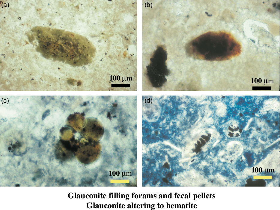
Fig. 3. Photomicrographs of glauconite- and pyrite-filled faecal pellets and foraminifera tests from the Shubuta Clay Member of the Yazoo Formation at St Stephens Quarry. (a) Glauconite-filled faecal pellet. (b) Glauconite-filled faecal pellet oxidized by weathering to haematite. (c) Glauconite- and pyrite-filled foraminifera with slight alteration to haematite. (d) Unoxidized pyrite-filled foraminifera (work from Ellwood et al. Reference Ellwood, Mcpherson, Sen Gupta and Matthews1986). These redox variations result in the colours observed in samples from these units throughout the SE United States.
The Shubuta Clay Member at the GM&O locality is ∼12 m thick and extends to the point where the gradient shallows and from there on the section is covered. Further to the east of our measured section, ∼200 m, exposed above a large slump, is a grey, tan to red, only slightly marly, silty to sandy sediment, locally containing very thin beds, slightly rich in carbonate. This unit reddens upwards and we are equating it to the upper ‘clay’ member that MacNeil (Reference MacNeil1944) has argued is the upper Red Bluff unit at the GM&O site. MacNeil suggested that this unit is the distal outwash of the Forest Hill delta to the west, but we equate this unit to the Red Bluff Formation of the Jackson Group.
3.b. Hiwannee outcrop section and core
A nearby section of ∼7 m thickness, located at the town of Hiwannee (HIW), Mississippi, ∼10 km south of Shubuta, was sampled (Fig. 1) (Dockery & Thompson, Reference Dockery and Thompson2011). The section was measured along the Chickasawhay River, where the top of the Shubuta Clay Member and base of the Red Bluff Formation are exposed. At this locality, the green glauconitic Shubuta Clay grades upwards into a bluish-appearing, phosphate-rich glauconitic marl (‘blue clay’ of Toulmin, Reference Toulmin1962). At this locality, above the river level, the exposed Shubuta Clay is ∼2 m thick, and the blue marl is ∼0.3 m thick and interpreted to be the basal member of the Red Bluff Formation. The change from the Shubuta Clay Member into the Red Bluff Formation above is fairly abrupt. The Red Bluff Formation is characterized by abundant pyrite-filled burrows, pyrite concretions and siderite nodules that are altered to various iron oxides and oxyhydroxides. The Red Bluff Formation here is a glauconite-rich, tan to brown, marly clay with pyritic burrows. This unit is interbedded with siderite-rich carbonate beds that weather out as siderite-rich iron-stained nodules. The section was covered above ∼7 m, as measured from the river level at that time.
Based on the disappearance of Hantkeninidae in this section, we place the E–O boundary in the HIW outcrop section at the base of the blue marl representing the base of the Red Bluff Formation. No Hantkeninidae specimens were found in the blue marl or in the rest of the Red Bluff Formation sampled above the blue marl.
In addition to the Chickasawhay River outcrop sampled at Hiwannee, we drilled and collected a core from the top of the river bluff, ∼500 m from the outcrop section. The core (Fig. 2b) penetrated ∼60 m of section, beginning with the Forest Hill Formation and ending in the North Twistwood Creek Formation. The Red Bluff Formation in the core appears to be separated from the Forest Hill Formation above by a disconformity. The E–O boundary lies at ∼24.2 m in the core and there is a gradational lithologic change through that interval, from the Shubuta Clay Member below to the Red Bluff Formation above (Fig. 4). A test of the gradational nature of this boundary is illustrated by the relatively smooth change in magnetic susceptibility data (χ) towards higher values in the Red Bluff Formation. This is an important test in cores, because sediment is often washed out owing to variations in bed hardness, and therefore an artificial ‘disconformity’ can inadvertently be created during the drilling process. To avoid such anomalies, we carefully examine core recovery versus the interval drilled, and collect and measure intervals where bedding changes occur to test for anomalous shifts in measured datasets. These include stable isotopes, on-core gamma ray measurement in the laboratory as compared to down-hole measurement, and χ. In the case of the HIW outcrop section and core, both are well correlated in terms of lithology and χ.
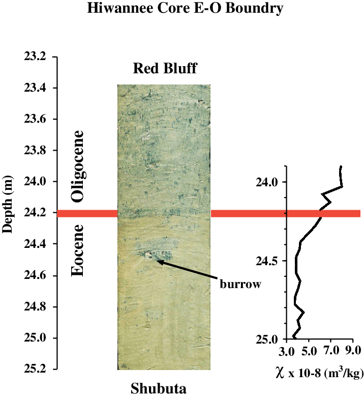
Fig. 4. A ∼2 m segment of core through the E–O boundary interval at Hiwannee, Mississippi, illustrating the colour changes from glauconitic to pyritic, and the gradational character in both the lithologic and χ datasets exhibited. These variations are similar to those seen in the SSQ ∼ 45 km to the southeast in Alabama.
3.c. St Stephens Pelham Hill North Quarry
Located at St Stephens Quarry (SSQ), SW Alabama (∼40 km southeast of the GM&O and HIW sections; Fig. 1), the SSQ measured section (Figs 2c, 5) contains abundant calcareous macro- and microfossils throughout. Here, we used a track-hoe to clean the quarry face at four localities along the quarry wall, so that unweathered, continuous surfaces were available for study. At the base of the section (measured from the Pelham Hill North Quarry floor) there is a glauconitic, pale blue-green, phosphate-rich, well-indurated marl that we identify as the Pachuta Marl Member of the Yazoo Formation. At ∼0.9 m, a disconformity (bold dashed line in Fig. 2c) contains a distinctively different macroinvertebrate fossil assemblage from that contained within the overlying Shubuta Clay Member. We equate this disconformity to the one we observe in the GM&O section (Fig. 2a). From ∼0.9 to ∼2.1 m in our SSQ measured section, the Shubuta Clay Member of the Yazoo Formation is exposed. At the base of the Shubuta Clay Member, and lying directly in contact with a disconformable surface below, are abundant carbonized wood fragments, some greater than 0.05 m in length, of an unknown species of tree. At the SSQ locality, the Shubuta Clay Member is a glauconitic, phosphatic marl, but darker grey-green than the underlying Pachuta Marl Member, and contains significantly less carbonate. At 1.6–1.8 m, a carbonate-rich bed within the Shubuta Clay Member, which we are informally calling the ‘Shubuta lime bed’ (Fig. 2c), provides an excellent marker horizon that we equate to the lower carbonate-rich bed we see in the GM&O section (Fig. 2a).
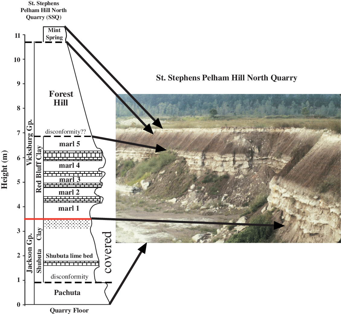
Fig. 5. St Stephens Pelham Hill North Quarry, near St Stephens, Alabama (SSQ, Figs 1, 2c), showing exposures of the Oligocene Red Bluff and Forest Hill formations, and Miocene Mint Spring Formation. Note that the Pachuta Marl and Shubuta Clay members of the Yazoo Clay Formation, Jackson Group, are covered intervals in the photograph and lie below the Red Bluff Formation. Stippled zone in the drawn section (left) represents the gradational transition from the Eocene Shubuta Clay Member into the Oligocene Red Bluff Formation, a zone in which Hantkeninidae diminish in size and disappear at the top. Note the light coloured interbedded marl–limestone couplets defining the Red Bluff Formation.
Above ∼2.1 m, we observe an increase in the abundance of pyrite-filled burrows, indicating a zone of condensed sediment accumulation and bioturbation (also observed in the GM&O section). Above this level, the Shubuta Clay Member is a carbonate-rich, greenish glauconite-rich clay/marl with some pyrite-filled burrows throughout. Where the Shubuta Clay Member is exposed to surface weathering (observed when sites are revisited at later times), glauconite has oxidized to maghaemite and haematite (Ellwood et al. Reference Ellwood, Mcpherson, Sen Gupta and Matthews1986; discussed briefly in the thermomagnetic Section 5.c below). In addition, weathering has produced abundant peds that formed Liesegang-type, tan discolourations as was observed within the Shubuta Clay Member at the GM&O locality.
At ∼3.55 m, the Shubuta Clay grades conformably into a fairly well-indurated grey marl unit equivalent to the blue marl in the HIW river section, the base of the Red Bluff Formation, and above that level, the unit exhibits alternating marl/limestone compositional changes (Fig. 6). When weathered, the unit better exhibits the characteristic and distinctive alternating limestone and marl sequences (Fig. 5). Perhaps the nomenclature problems result from the fact that previous authors have assigned a variety of names to this unit, leading to some confusion in the literature. For example, this unit has been called the Red Bluff Member of the Forest Hill Formation, the Red Bluff Formation, the Red Bluff Clay and the Bumpnose Limestone (e.g. MacNeil, Reference MacNeil1944; Murray, Reference Murray1947, Reference Murray1952; Toulmin, Reference Toulmin1955; Waters & Mancini, Reference Waters and Mancini1982, Coleman, Reference Coleman1983; Mancini & Waters, Reference Mancini and Waters1986; J. A. Bryan, unpub. Ph.D. dissertation, Univ. Tennessee, 1991; Tew & Mancini, Reference Tew and Mancini1992; Miller et al. Reference Miller, Thompson and Kent1993, Mancini, Reference Mancini2000), and part of the Shubuta Clay Member (Bybell & Poore, Reference Bybell and Poore1983; Keller, Reference Keller1985). This unit is lithologically similar to the Red Bluff Formation exposed in outcrop along the Chickasawhay River (HIW outcrop and core). After careful study of all our sections, we are calling this unit the Red Bluff Formation (pictured in outcrop in Fig. 5 and drawn in Fig. 2c) of the Vicksburg Group. The basal Red Bluff Formation is a dark grey phosphatic marl that grades upwards into a bluish-grey to white, phosphatic semi-massive limestone, alternating with marl lenses, and with local occurrences of glauconite (Fig. 6). The Red Bluff Formation is very different from the type Bumpnose Limestone Member of the Ocala Formation (Moore, Reference Moore1955) exposed near Marianna, Florida (Figs 2e, 7).
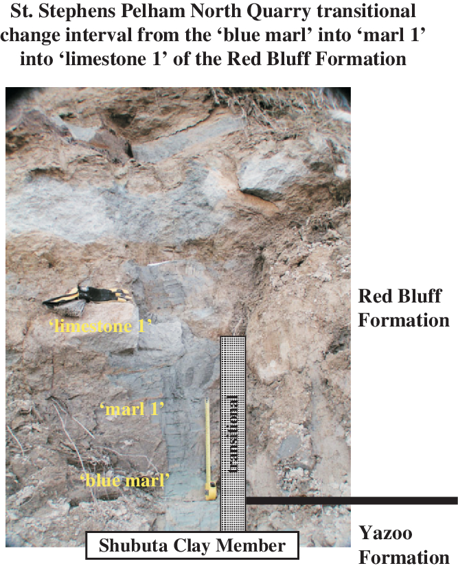
Fig. 6. The gradational transition in the St Stephens quarry from the glauconite-rich Shubuta Clay Member of the Yazoo Formation into the overlying darker specular pyrite-abundant Red Bluff Formation with the ‘blue marl’ colour variant at its base. Also shown are ‘marl 1’ and ‘limestone 1’ of the Red Bluff Formation (Fig. 2b). Tape measure for scale is extended 56 cm.

Separating the uppermost Red Bluff Formation from the overlying Forest Hill Formation, at ∼6.7 m in our measured SSQ section, is the second of only two disconformities in the succession. In the SSQ, we place the E–O boundary at the top of the Shubuta Clay Member, base of the Red Bluff Formation, and therefore at the base of the Vicksburg Group. This is based on identification of Hantkeninidae in samples collected through the Shubuta Clay Member, with the highest observed occurrence point (HOOP) of Hantkeninidae at the base of the Red Bluff Formation, identified as ‘blue marl’ in Figure 2c, and equivalent to the base of the blue marl at Hiwannee.
3.d. Red Stick Quarry
The Red Stick Quarry (RSQ) is located near Claiborne, Alabama, ∼53 km east of St Stephens, Alabama (Fig. 1). Exposed here are the upper Pachuta Marl and Shubuta Clay members of the Yazoo Formation (Fig. 2d), and the Red Bluff Formation of the Vicksburg Group. The E–O boundary is identified based on the HOOP of Hantkeninidae, and that level is denoted with a solid red line in Figure 2d. Here, the marl intervals in the Red Bluff Formation are better defined and thicker than in the SSQ section, with limestone elements occurring as thin beds within the thicker marls. Again, the Red Bluff Formation does not resemble the glauconitic Bumpnose Member of the Ocala Limestone whose type locality is in the Brooks Quarry near Marianna, Florida (Fig. 7; described in Section 3.e below).
The Pachuta Marl (∼0.5 m thick) and Shubuta Clay (∼1.8 m thick) members of the Yazoo Formation are exposed in the RSQ in a fairly steeply eroded bench. This bench extends upwards into the Red Bluff Formation, ∼0.8 m, where the angle of the bench begins to flatten. Above that level, the Red Bluff is deeply penetrated by weathering resulting in significant pedogenic alteration of the section. A unique aspect of the RSQ is that the section contains abundant phosphate, with phosphatized sponges and other macrofossils. In the SSQ, phosphate occurs in the Pachuta and Shubuta members and Red Bluff Formation, but the abundance of phosphate at RSQ is significantly higher.
3.e. Brooks Quarry
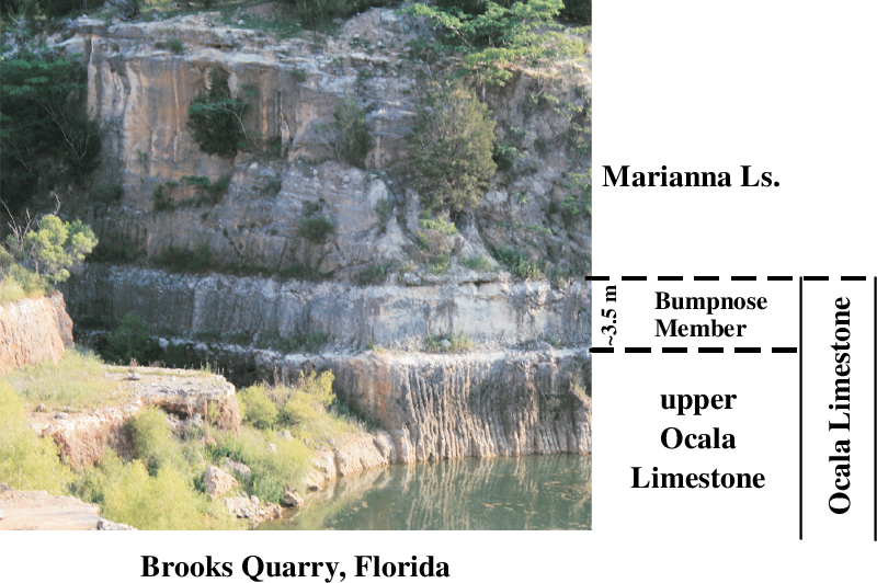
The Brooks Quarry (BQ) complex near Marianna, Florida (Fig. 1), is located ∼270 km southeast of St Stephens, Alabama, and is near the type locality for the Bumpnose Member of the Ocala Limestone as defined by Moore (Reference Moore1955). This relatively massive, densely fossiliferous packstone/grainstone, locally granular, less well-indurated unit is so distinctive that it is easily identified within the quarry (Fig. 7). The Bumpnose Member in the type area is lithologically distinct from any named equivalent in the SSQ and RSQ as described above.
At the base of the BQ section, the upper part of the Ocala Limestone is very similar in character (lithology, texture and some fauna) to its Bumpnose Member, but is separated from the Bumpnose Member by an easily identified disconformity (Fig. 2e). The Eocene Asterocyclina Zone (Fig. 2), previously considered to be restricted to the upper Ocala Limestone, extends into the Bumpnose Member, across the disconformity defining the base of that unit. While previous studies placed the Bumpnose Member within the Oligocene, we now place the base of the Bumpnose Member within the Eocene. This is based on the occurrence at ∼2.15 m in the BQ measured section, within the Bumpnose Member, of a specimen of Asterocyclina americana (Cushman) found in situ (Specimen HVH 12716, now in the H. V. Howe Type Collection of Microfossils at Louisiana State University; Fig. 2, upper right). In addition, specimens of Hantkeninidae were also recovered in the lower Bumpnose Member, indicating that the E–O boundary lies between 2.5 to 3.1 m in our measured section. We place the E–O boundary at ∼2.55 m using χ data. From ∼2.8 m to ∼4.55 m, the Bumpnose Member is quite friable, above which the unit again becomes much more indurated. There is a disconformable boundary between the Bumpnose Member of the Ocala Limestone and the overlying Oligocene Marianna Limestone. This base of the Marianna Limestone at the BQ exhibits lithologic similarities to the Mint Spring Formation, observed immediately overlying the Forest Hill Formation at the SSQ locality (Figs 2c, 5). The Marianna Limestone begins at ∼5.55 m within the BQ measured section (Fig. 2e).
3.f. General lithostratigraphic discussion for all successions studied
Successfully correlating units that span the E–O boundary in the SE United States Gulf Coast has been complicated by long-standing misinterpretations introduced and perpetuated in the literature. For instance, Murray (Reference Murray1947) defined the Shubuta Clay based on exposures at Shubuta, Mississippi, and placed the unit within the Yazoo Formation. However, at the Red Bluff GM&O section (Hilgard, Reference Hilgard1860), only ∼1.3 km away, the Shubuta Clay was reported as equivalent to the younger Forest Hill Formation (MacNeil, Reference MacNeil1944). As a consequence, the Shubuta Clay could either be reassigned as a member within the Forest Hill Formation, or as the lower portion of the originally defined Red Bluff Clay sequence at the GM&O trestle, or could be part of the Yazoo Formation. Based mainly on lithologies and the extinction of Hantkeninidae, we place the E–O boundary at the top of the Shubuta Clay Member of the Yazoo Formation. As shown in Figure 6, the Shubuta Clay is gradational into the overlying Red Bluff Formation, the basal unit of the Vicksburg Group (Fig. 2).
We interpret the upper and lower disconformities in both the SSQ and BQ to be correlated (Fig. 2). Based on interpretation of benthic foraminifera (B. S. Gupta, Louisiana, pers. comm. to B. Ellwood), the SSQ generally represents deposition in deeper water than does the outer carbonate bank BQ sequence to the southeast. Therefore, the erosion that formed these disconformities would have commenced first in the shallower-water outer-shelf carbonate bank environment of the BQ area, forming the basal erosional surface at BQ, and then later at the deeper-water SSQ locality to the WNW (Fig. 1). Likewise, it was expected that as sea-level recovered, deposition would begin first at SSQ and later at BQ. The result is that through this interval, more section is expected to be missing in the disconformities at BQ than at SSQ. Given the thick succession represented by the GM&O and HIW sections, even though these sections were closer to shore, accommodation space at GM&O and HIW was greater than at either the SSQ or BQ localities. This correlation is based on the E–O boundary being bracketed by disconformities in both the SSQ and BQ sections and by age-equivalent biozones and χ datasets (presented in Sections 4–6 below).
4. General biostratigraphic discussion
The Eocene–Oligocene Series boundary is defined based on the last appearance datum (LAD) of the family Hantkeninidae at the 19 m level in the Massignano GSSP Section near Ancona, Italy (Premoli-Silva & Jenkins, Reference Premoli-Silva and Jenkins1993; Jovane et al. Reference Jovane, Coccioni, Marsili, Acton, Koeberl and Montanari2009), and is a global marker for the end of the Eocene. This LAD is closely preceded by the HOOPs of Turborotalia cunialensis and Turborotalia cocoaensis. Both species are found in samples collected from the SSQ and BQ sections, and Hantkeninidae were present in all successions sampled for this paper. The point of disappearance of Hantkeninidae was used to assign the E–O boundary location, represented by the solid red lines in Figure 2a–e. Biostratigraphy for the five sampled sections is discussed below.
4.a. Red Bluff type locality (GM&O; Fig. 2a)
Seven samples were collected for biostratigraphic analysis through the ∼13 m of section exposed at the GM&O railroad trestle and these were examined for Hantkeninidae. All samples from the section contained Hantkeninidae specimens. Therefore, we assign all but the very top of the GM&O section, which was not sampled because it is deeply covered, to the Eocene (Fig. 2a).
4.b. Hiwannee locality (HIW; Fig. 2b)
Because of the large volume of sample material needed for the biostratigraphic analysis, these samples were collected from the outcrop section located on the Chickasawhay River, and not from the well-correlated core. Five samples for biostratigraphic analysis were collected at the HIW outcrop section, two from the Shubuta Clay Member, one from the blue marl (a colour variant at the base of the Red Bluff Formation) and two from the upper part of the Red Bluff Formation. Each was examined for Hantkeninidae. In samples from the Shubuta Clay, we were able to identify Hantkeninidae in both samples. No Hantkeninidae specimens were found in the blue marl or in Red Bluff Formation samples, nor were specimens of T. cunialensis and T. cocoaensis, the other Eocene marker species common in these sections. Therefore, we place the boundary at the transition from the Shubuta Clay into the blue marl in this section (Fig. 2b).
4.c. St Stephens Quarry locality (SSQ; Figs 2c, 5)
Placement of the E–O boundary at the St Stephens Pelham Hill North Quarry locality in previous biostratigraphic studies has varied (e.g. Waters & Mancini, Reference Waters and Mancini1982; Bybell & Poore, Reference Bybell and Poore1983; Mancini & Waters, Reference Mancini and Waters1986; Miller et al. Reference Miller, Thompson and Kent1993; Keller, Reference Keller1985), in part owing to lithostratigraphic uncertainties as discussed in Section 3.c above. In our work, we identified numerous Hantkeninidae within the Pachuta Marl and Shubuta Clay members, but none were found in the lowermost portion of the Red Bluff Formation (Fig. 2c). We also found that above ∼2.0 m in our measured section, the abundance and size of Hantkeninidae in the Shubuta Clay Member rapidly dropped, a pre-extinction dwarfing-type effect (Wade & Olsson, Reference Wade and Olsson2009) occurring before the final E–O extinctions. This level is approximately equivalent to that identified by Waters & Mancini (Reference Waters and Mancini1982) and Mancini & Waters (Reference Mancini and Waters1986) as the E–O boundary. The drop in size and abundance of Hantkeninidae in our samples may also explain why Miller et al. (Reference Miller, Thompson and Kent1993, Reference Miller, Browning, Aubrey, Wade, Katz, Kulpecz and Wright2008) were not able to resolve the boundary level from core samples, and thus they placed the boundary near the base of the Shubuta Clay Member using lithostratigraphic criteria. They also placed an unconformity between the Shubuta Clay Member and Red Bluff Formation, which we argue was most probably the result of core wash-out effects due to drilling through alternating limestone/marl, hardground/softground. Rather, this lithologic boundary is clearly gradational (Fig. 6). This result is supported by the work of Fluegeman (Reference Fluegeman, Demchuk and Gary2009), where he argues that the foraminiferal data from Little Stave Creek, ∼10 km from the SSQ succession, indicate that the Shubuta Clay Member – Red Bluff Formation contact is conformable.
4.d. Palynomorph assemblages from St Stephens Quarry
Palynomorph assemblages from SSQ samples exhibit good to excellent preservation and are dominated by dinoflagellate cysts. Homotryblium sp. and the Spiniferites group were consistently found throughout the samples in high to moderate abundances. In addition, organic linings of foraminiferal tests were present throughout the entire section along with terrestrial pollen and spores, which represent a small percentage of the overall assemblage.
The Pachuta Marl Member disconformity is dominated by a peak in foraminiferal linings and terrestrial pollen, namely undifferentiated bisaccates and Momipites sp. This influx in terrestrial palynomorphs is followed by an acme of Homotryblium floripes at 1.54–1.936 m within the Shubuta lime bed at ∼1.65 m (Fig. 2c). These taxa are common in tropical, estuarine environments and may prove useful as a correlation event across the upper Eocene elsewhere in the SE United States. The middle Shubuta Clay Member contains the lowest observed occurrence point (LOOP) of Enneadocysta multicornuta and Membranophoridium aspinatum, in samples 1.629 m and 1.936 m, respectively, suggesting a Priabonian age (Brinkhuis, Reference Brinkhuis1994; Jaramillo & Oboh-Ikuenobe, Reference Jaramillo, Oboh-Ikuenobe, Goodman and Clarke2001). This age interpretation is further supported by the presence of late Eocene taxa Corrudinium incompositum and Operculodinium divergens and the HOOP of Wetzeliella gochtii and LOOP of Wetzeliella symmetrica. The highest observed rare occurrence Point (HOROP) of Heteraulacacysta porosa is seen at 2.288 m indicating a late Priabonian age in the upper Shubuta Clay Member (Edwards, Reference Edwards, Ward and Krafft1984; Head & Norris, Reference Head, Norris, Srivastava, Arthur, Clement, Aksu, Baldauf, Bohrmann, Busch, Cederberg, Cremer, Dadey, de Vernal, Firth, Hall, Head, Hiscott, Jarrard, Kaminski, Lazarus, Monjanel, Nielsen, Stein, Thiébault, Zachos, Zimmerman and Stewart1989).
Identification of the E–O boundary, using dinoflagellate cysts and palynomorph assemblages, is somewhat problematic. Van Mourik & Brinkhuis (Reference Van Mourik and Brinkhuis2005) argued for the top, HOOP, of Areosphaeridium diktyoplokum as the global palynological marker for the boundary. This taxon, however, is not documented at SSQ. Therefore, alternative taxa must be applied. K. Jensen (unpub. M.S. thesis, Louisiana State Univ., 2012) proposed the LOOP of Nematosphaeropsis cf. lemniscata as an E–O boundary marker, which he identified at 3.65 m in SSQ samples. Jaramillo & Oboh-Ikuenobe (Reference Jaramillo and Oboh-Ikuenobe1999, Reference Jaramillo, Oboh-Ikuenobe, Goodman and Clarke2001) noted an overall increase in Deflandrea phosphoritica and in a condensed interval they identified as the Shubuta Clay Member – Red Bluff Formation contact. The SSQ record of increases in the Deflandrea group, also observed in our study, can be divided into several events. The initial increase in D. phosphoritica occurs at 3.608 m (Fig. 2c), and is seen in conjunction with a maximum increase in Wetzeliella symmetrica. Highest abundances of D. phosphoritica and D. heterophlycta are documented at 4.3–4.7 m, representing a high-nutrient, more near-shore environment in earliest Oligocene times (Kothe, Reference Kothe1990; Brinkhuis et al. Reference Brinkhuis, Powell, Zevenboom, Head and Wrenn1992). In addition, the HOOPs for dinoflagellate species, Corrudinium incompositum at 4.0 m and Diphyes colligerum at 4.3 m, are within, or approximately coincident with their established ranges elsewhere, with range tops in the lowermost Rupelian (Head & Norris, 1989; Williams et al. Reference Williams, Stover and Kidson1993). All of these data are consistent with the boundary pick given here using the Hantkeninidae HOOP (Fig. 2c).
4.e. Red Stick Quarry locality (RSQ; Fig. 2d)
Using biostratigraphic analysis for RSQ samples we identify the planktonic foraminifera Hantkeninidae, T. cocoaensis and T. cunialensis within the Pachuta Marl and Shubuta Clay members of the Yazoo Formation, with a HOOP for T. cunialensis at 1.7 m, a HOOP for T. cocoaensis at 1.8 m and a HOOP for Hantkeninidae above 2.0 m. The next sample analysed was at 2.15 m in the section and none of these Eocene marker species were present at this level or in samples above. Therefore, we have placed the E–O boundary level at 2.08 m in the RSQ section at the base of Red Bluff Formation ‘marl 1’ (Fig. 2d). Larger foraminifera are also present, and support the planktonic foraminiferal data. The Pachuta Marl Member has a typical late Eocene assemblage of Pseudophragmina bainbridgensis, Lepidocyclina cf. L. ocalana, Nummulites marianensis, Nummulites floridensis and Nummulites willcoxi. A zone rich in phosphate in the upper Shubuta Clay Member also has rare Nummulites floridensis. The basal Oligocene Red Bluff Formation contains rare Lepidocyclina chaperi, which are common in the Bumpnose Limestone of the BQ and equivalent facies in the Florida peninsula, and is typical of lower Oligocene rocks in the Gulf Coast. The Red Bluff Formation also contains the oyster Lopha vicksburgensis, another index taxon for the lower Oligocene of the eastern Gulf Coast region.
4.f. Brooks Quarry (BQ; Figs 2e, 7)
Our preliminary biostratigraphic interpretations, based on finding Asterocyclina americana in the Bumpnose Member of the Ocala Limestone in the BQ section (insert in Fig. 2), indicated that at least the basal ∼0.1 m of the Bumpnose Member is Eocene. Using planktonic foraminifera, specifically the Eocene marker fauna Hantkenina alabamensis and Turborotalia cerroazulensis (Fig. 8), and χ data allows us to place the E–O boundary at ∼2.55 m above the base of our measured section (Fig. 2e).
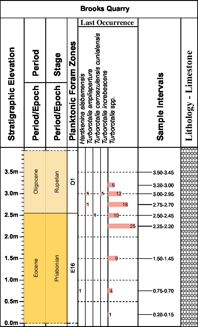
Fig. 8. Planktonic foraminiferal stratigraphic distribution for samples from the Brooks Quarry (BQ) measured section. Horizontal shaded bars represent histograms of abundances. The number of organisms identified is included.
5. Magnetic susceptibility (χ) methods
5.a. Magnetostratigraphic susceptibility: brief comments
All materials are ‘susceptible’ to becoming magnetized in the presence of an external magnetic field, and initial low-field bulk mass-specific magnetic susceptibility (χ) is an indicator of the strength of this transient magnetism. χ is very different from remanent magnetism (RM), the intrinsic magnetization that accounts for the magnetostratigraphic polarity of materials. χ in marine stratigraphic sequences is generally considered to be an indicator of detrital iron-containing paramagnetic and ferrimagnetic grains, mainly ferromagnesian and clay minerals (Bloemendal & De Menocal, Reference Bloemendal and De Menocal1989; Ellwood et al. Reference Ellwood, Crick, El Hassani, Benoist and Young2000, 2008a; da Silva & Boulvain, Reference da Silva and Boulvain2002, Reference da Silva and Boulvain2005), and can be quickly and easily measured on small, unoriented or friable samples.
Low-field bulk mass-specific magnetic susceptibility, as used in most reported studies, is defined as the ratio of the induced moment (Mi or Ji) to the strength of an applied, very low-intensity magnetic field (Hj), where
 $${{\rm{J}}_{\rm{i}}} = {\chi _{{\rm{ij}}}}{{\rm{H}}_{\rm{j}}}\left ({{\rm{mass}} - {\rm{specific}}} \right)$$
(1)
$${{\rm{J}}_{\rm{i}}} = {\chi _{{\rm{ij}}}}{{\rm{H}}_{\rm{j}}}\left ({{\rm{mass}} - {\rm{specific}}} \right)$$
(1)
or
 $${{\rm{M}}_{\rm{i}}} = {{\rm{\kappa}} _{{\rm{ij}}}}{{\rm{H}}_{\bf{j}}}.{\rm{}} \left ({{\rm{volume}} - {\rm{specific}}} \right)$$
(1)
$${{\rm{M}}_{\rm{i}}} = {{\rm{\kappa}} _{{\rm{ij}}}}{{\rm{H}}_{\bf{j}}}.{\rm{}} \left ({{\rm{volume}} - {\rm{specific}}} \right)$$
(1)
In these expressions, magnetic susceptibility in SI units is parameterized as κ, indicating that the measurement is relative to a one cubic metre volume (m3) and therefore is dimensionless; magnetic susceptibility parameterized as χ indicates measurement relative to a mass of one kilogram, and is given in units of m3/kg. Both χ and κ are tensors of the second rank and therefore have anisotropy. To reduce the effect of anisotropy in bulk measurement, all samples are broken up in the laboratory to disrupt anisotropic effects.
χ measurements are reported in this paper for samples from three of the six sections sampled: SSQ (Figs 9–11), BQ (Fig. 10) and HIW (core and outcrop Figs 4, 12). These samples were collected from cleaned successions and core where the glauconite present did not show alteration to maghaemite or haematite. κ (Fig. 13) from thermomagnetic measurement is used to characterize carriers of the magnetic susceptibility, and these data are discussed below.
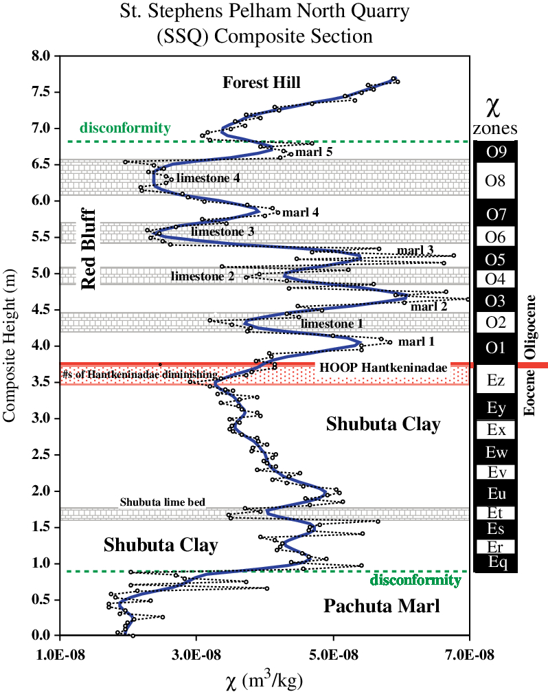
Fig. 9. Low-field bulk mass-specific magnetic susceptibility (χ) data for the St Stephens Pelham Hill North Quarry measured composite section. χ is reported as raw (dotted curve) and smoothed (solid curve) datasets; circles represent stratigraphic position of each sample collected. Lithology corresponding to Figures 2c and 5. χ bar-log zonation is constructed from the smoothed χ dataset, and χ zones are labelled: ascending through the Oligocene (O1–O9) and descending through the Eocene (Ez–Eq). The E–O boundary is represented by the solid red line and is identified by the HOOP (highest observed occurrence point) of Hantkeninidae, and lies at the top of the conformable transition from the Shubuta Clay Member into the Red Bluff Formation where Hantkeninidae diminish in size and at the top disappear from the section. Note that there is a disconformity between the Pachuta Marl Member and the Shubuta Clay Member identified by a distinctive hardground, wood fragments and a large change in the χ dataset. Based on an abrupt shift in the χ dataset, a second disconformity may exist between the top of the Red Bluff Formation and the overlying Forest Hill Formation.
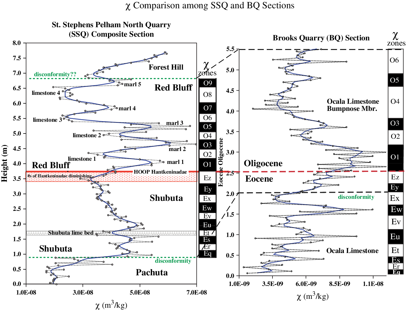
Fig. 10. Lithologic and χ comparison between the SSQ and BQ sections (Figs 1, 2c, e). The solid red line in the SSQ data represents the E–O boundary, picked using the HOOP for Hantkeninidae; the dashed red line in the BQ represents a pick from both biostratigraphy and χ correlation. The disconformity between the Shubuta and Pachuta beds in the SSQ is observed higher in the BQ section. χ data bar-logs were constructed from smoothed χ datasets from both quarries. Note that a number of the Oligocene χ zones present at SSQ are missing in the BQ.
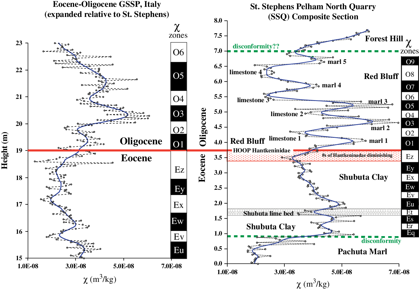
Fig. 11. Comparison of χ bar-log data from the SSQ section versus the GSSP at Massignano, Italy (χ zones as in Fig. 9). Note the similar range of χ values among the two sections. The solid red line represents the E–O boundary location in these two successions. χ data for the GSSP are modified from Jovane et al. (Reference Jovane, Florindo, Sproviere and Pälike2006, Reference Jovane, Sprovieri, Florindo, Acton, Coccioni, Dall’Antonia and Dinarés-Turell2007).
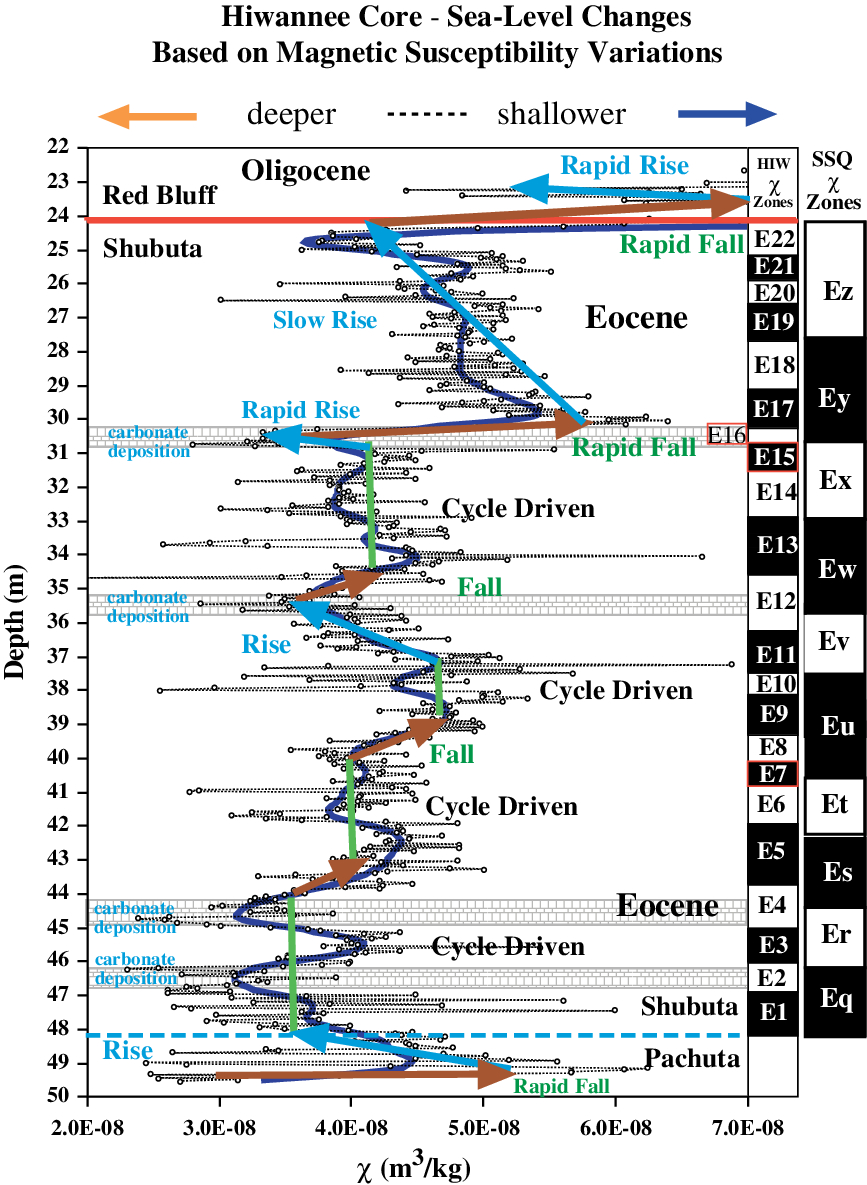
Fig. 12. The χ dataset for the Eocene segment of the Hiwannee (HIW) core, illustrating cyclic trends and shallow versus deeper-water fluctuations represented in a ∼24 m segment of core. HIW bar-logs are compared to SSQ bar-logs (right) and indicate that the Shubuta SAR at Hiwannee is approximately double that represented by the Eocene SSQ sequence sampled. The rise and fall nomenclature is interpreted as sea-level variations during deposition of this sequence. Note that when sea-level is interpreted as deeper, there is carbonate deposition as indicated by CaCO3-rich levels in the core. These are similar to the high carbonate ‘Shubuta lime bed’ observed in St Stephens Quarry (Figs 2a, c, 9–11, 17).
5.b. Field sampling
Measured outcrop sections in Figure 2 were carefully cleaned until fresh outcrop material was available for sampling. In the case of SSQ sections, a track-hoe was used to clean multiple sections. Samples for χ were collected at 0.05 m intervals. At the SSQ locality (Fig. 2c), a composite section was constructed using 165 samples for which χ was measured (Fig. 9). A total of 110 samples were collected from the BQ section for which χ was measured (Fig. 10). Nine of these samples were chosen for foraminiferal studies, with samples from the Bumpnose Member of the Ocala Limestone taken at 0.25 m intervals.
5.c. Laboratory measurement
Laboratory χ measurements reported in this paper were performed using the Williams susceptibility bridge at Louisiana State University (LSU), calibrated relative to mass using standard salts reported by Swartzendruber (Reference Swartzendruber1992) and CRC tables. We report χ in terms of sample mass because it is much easier and faster to measure with high precision than is volume, and it is now the standard for χ measurement. The Williams low-field χ bridge can measure diamagnetic samples at least as low as −4 × 10⁻⁹ m3/kg. This is illustrated by two relatively pure calcite samples collected from a 3 m core drilled from a standing, isolated speleothem in Carlsbad Caverns National Park, with measured values and standard deviation for three replicate measurements of CA-1 =−3.37 ± 0.08 × 10⁻⁹ m3/kg, and CA-2 = −3.46 ± 0.09 × 10⁻⁹ m3/kg. These samples are used as measurement standards.
Thermomagnetic susceptibility measurements (TSM, values measured as κ), using the KLY-3S Kappa Bridge at LSU, were performed to characterize the type of mineral responsible for the κ signal. This measurement involves heating a sample from room temperature to 700 °C while measuring κ as the temperature rises and falls. Paramagnetic-type minerals show a parabolic-shaped κ decay during this process, because κ in these samples is inversely proportional to temperature of measurement (Hrouda, Reference Hrouda1994). Ferrimagnetic-type minerals, on the other hand, usually show an increase in κ up to a point where κ decays towards the Curie/Neel temperature of the minerals responsible for κ. In the case of magnetite this temperature is ∼580 °C. Previous work reported on standard illite samples shows an initial paramagnetic phase, interpreted to be illite with TSM values below 10, that then begins to convert to ferrimagnetic magnetite at temperatures near or above 400 °C (Ellwood et al. Reference Ellwood, Brett and Macdonald2007). Such conversion peaks are common in TSM datasets (e.g. Fig. 13).
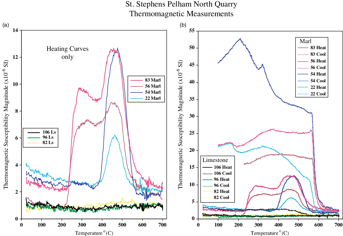
Fig. 13. Thermomagnetic susceptibility (TSM, κ v. T) results for measurements of Shubuta Clay Member and Red Bluff Formation limestone and marl samples from the SSQ section: (a) heating curves only; (b) heating and cooling both reported.
Samples from the SSQ section exhibit some interesting changes. All samples measured have a low initial κ magnitude and exhibit behaviour typical for κ dominance by paramagnetic constituents: decreasing values with increasing temperature from room temperature up to ∼200 °C (Fig. 13a). Had these samples been weathered, we would expect to see the inverse: a ferrimagnetic component in the initial heating curves that would reflect the development of maghaemite that then converts to haematite in the sample, shown to be produced during weathering (Fig. 3; Ellwood et al. Reference Ellwood, Mcpherson, Sen Gupta and Matthews1986). At higher temperatures, the curve changes to give an indication of the changes in iron mineralogy. Therefore, it appears that the samples measured were not altered by weathering prior to measurement, because ferrimagnetic maghaemite does not contribute to the initial κ values. In addition, the samples showed a green glauconitic colour that when exposed in outcrop acquires a brown discolouration due to the conversion of glauconite to maghaemite. During heating, the SSQ marl samples exhibit conversion peaks to ferrimagnetic magnetite, with Curie temperatures at ∼580 °C, resulting in large increases in κ during cooling (Fig. 13b). We attribute the unusual double peaks exhibited by three of the marl samples, with breakdown and conversion beginning at ∼200 °C, a trough at ∼350–400 °C and then a further increase in κ to ∼450 °C (Fig. 13a), to the breakdown of glauconite to magnetite in the laboratory. The second peak represents secondary magnetite exhibiting a strong κ in the measuring field above 450 °C, after which κ decreases to its Curie point. At high temperatures, some samples exhibit maghaemite (∼610 °C) and haematite (∼680 °C) Curie/Neel points indicative of conversion, during sample heating, to these iron oxide phases (e.g. no. 83 marl in Fig. 13a). Figure 13a only shows the heating curves, while Figure 13b shows both the heating and cooling curves for the samples reported here. Note, the large increase in κ that results from the breakdown of the dominant paramagnetic minerals to the resulting ferrimagnetic components produced in these samples causes large acquisition of a magnetic signal in these samples after heating.
5.d. Presentation of χ data
Two χ data formats are presented in Figure 9, with both the raw data (dotted lines with data points indicating stratigraphic position) and smoothed data (solid curve), plotted on a linear scale. For presentation purposes and inter-dataset comparisons, the bar-log format, similar to that previously established for magnetostratigraphic polarity data presentations, is used here. Bar-logs are constructed from χ data that were smoothed using splines to hold data points in stratigraphic position (splines were calculated using the JMP statistical software package from the SAS Institute, Inc.). Splines vary depending on the number of samples in each dataset, and therefore, as with other smoothing techniques, the selection of splines is somewhat subjective. Comparison among χ datasets for the SSQ and BQ sections are given in Figure 10.
Because χ data in many cases have been shown to be cyclic (e.g. Mead et al. Reference Mead, Tauxe and Labrecquel1986; Hartl et al. Reference Hartl, Tauxe and Herbert1995; Weedon et al. Reference Weedon, Shackleton, Pearson, Shackleton, Curry, Richter and Bralower1997, Reference Weedon, Jenkyns, Coe and Hesselbo1999; Shackleton et al. Reference Shackleton, Crowhurst, Weedon and Laskar1999; Crick et al. Reference Crick, Ellwood, El Hassani, Hladil, Hrouda and Chlupac2001; da Silva & Boulvain, Reference da Silva and Boulvain2005; Jovane et al. Reference Jovane, Florindo, Sproviere and Pälike2006; De Vleeschouwer et al. Reference De Vleeschouwer, da Silva, Boulvain, Crucifx and Cllaeus2011; Luu et al. Reference Luu, Ellwood, Tomkin, Nestell, Nestell, Ratcliffe, Rowe, Huyen, Nguyen, Nguyen, Nguyen and Dao2018; Benedetti et al. Reference Benedetti, Haws, Bicho, Friedl and Ellwood2019), for the purpose of correlating among geological sequences, we use the bar-log plotting convention, such that if a χ cyclic trend is represented by two or more data points, then this trend is assumed to be significant and the highs and lows associated with these cycles are differentiated by black (high χ values) or white (low χ values) bar-logs (examples are shown in Figs 9–12). This method produces the best results when large numbers of closely spaced samples are being analysed. Such high-resolution datasets help resolve χ variations associated with anomalous samples, like those resulting from weathering effects, secondary alteration and metamorphism. Variations in χ may also be associated with long-term trends due to factors such as eustacy, as opposed to shorter-term climate cycles (Ellwood et al. Reference Ellwood, Tomkin, Febo and Stuart2008 b), or event sequences such as impacts (Font et al. Reference Font, NéDélee, Ellwood, Mirão and Silva2011). In addition, variations resulting from different sediment sources or sediment types can be resolved by developing and comparing bar-logs among localities. This is shown in Figure 11, where χ bar-logs from the E–O GSSP data from friable, relatively pure limestone samples are compared to χ derived bar-logs from the SSQ mainly clay and marl sediments.
5.e. Discussion of χ data
The SSQ composite section exhibits a distinctive cyclic χ signature (Fig. 9). The Pachuta Marl Member generally has low χ values, due to the high carbonate content and correspondingly low detrital component. However, χ makes a major jump in values across the disconformity between the Pachuta Marl and Shubuta Clay members. This disconformity was the result of subaerial exposure at the site when sea-level fell towards the end of the Eocene Epoch, as evidenced by an irregular erosional surface, significant horizontal lithological differences across the surface and the accumulation of large wood fragments (some over 0.07 m long) and other debris lying on a hardground between the Pachuta Marl and Shubuta Clay members. In the upper Shubuta Clay Member, transgression reaches a maximum, reflected by the lowest χ values, and regression starts at the point where the section transitions from the Shubuta Clay Member into the Red Bluff Formation interval (at ∼3.5 m in Fig. 9).
The χ signature seen in the SSQ section is also observed in the BQ section, although it is not as well defined (Fig. 10). The BQ χ data are an order of magnitude lower than at SSQ, because the limestone at BQ has a very low concentration of detrital grains due to its isolation in an outer carbonate bank. Nevertheless, χ cyclicity is preserved and the bar-log graphic comparison allows correlation among sections as well as evaluation of the extent of missing time at erosional surfaces that are common among these sections (Fig. 10).
Direct comparison to the Massignano GSSP in Italy is also possible using the LAD of Hantkeninidae at Massignano (Jovane et al. Reference Jovane, Sprovieri, Florindo, Acton, Coccioni, Dall’Antonia and Dinarés-Turell2007), the HOOP at SSQ and χ cyclicity (Fig. 11). Bar-logs developed for the SSQ and Massignano GSSP section χ datasets are presented in Figure 11 and graphically compared in Figure 14. χ cycles are well correlated among these successions, with the GSSP representing a slightly higher estimated residual sediment accumulation rate (SAR) than is observed at SSQ (Fig. 14). The 26° angle observed for the line of correlation (LOC) in Figure 14 indicates that the SAR for the GSSP is significantly higher relative to the SSQ rates. The relatively low scatter of points defining the LOC in Figure 14 shows that the LOC is well constrained, with a slight, longer frequency transgressive–regressive (T–R) eustatic cyclicity superimposed on the two datasets.
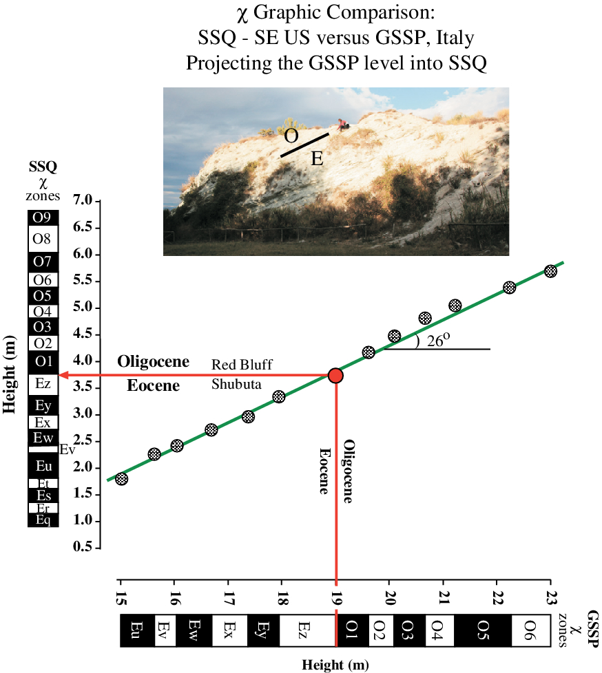
Fig. 14. Graphic comparison of χ bar-logs between the GSSP (shown in insert -top) and SSQ datasets. Data points are the intersection of each SSQ χ zone top and base with the corresponding χ zone top and base in the GSSP. A single line of correlation (LOC) is fit through these data. The 26° angle represents the angle of the LOC to the GSSP dataset and being less than 45° indicates that sediment accumulated faster at the GSSP section relative to the SSQ section. Graphic comparison produces a well-defined straight-line segment indicating that the two datasets represent similar amounts of time. The E–O boundary at the GSSP is identified by the last appearance datum (LAD) of the Hantkeninidae family, corresponding in the SSQ to the HOOP of Hantkeninidae that coincides with the transition from the Shubuta Clay Member to the Red Bluff Formation in the SSQ. This transition lies at the beginning of χ zone O1 in both sections.
Graphic comparison between the equivalent χ zones from SSQ and BQ (Fig. 10) demonstrates that there is a significant amount of the BQ section missing relative to the SSQ section. The Shubuta Clay Member, above the disconformity at SSQ, includes half-cycles Eq to Ez. However, much of this interval is missing in the BQ sequence and sedimentation only resumes in χ Zone Ey, shortly before the estimated E–O boundary at BQ (Fig. 10). In addition, half-cycles O7 to O9 are missing in the BQ section (Fig. 10). At the GM&O section, which is much closer to the E–O boundary shoreline, SAR begins to dramatically increase, with the remaining Shubuta Clay Member over 11 m thick (Fig. 2a).
We observe that Hantkeninidae abundance decreases above the Shubuta lime bed, in χ Zone Et at SSQ (Fig. 9), with the complete disappearance of Hantkeninidae at the end of Ez. The time leading up to the diminishing Hantkeninidae numbers also represents a decreasing χ trend, indicative of a period of gradual sea-level rise and gradual transgression due to corresponding ocean expansion during a global warming period. These trends abruptly shift just before the E–O boundary towards gradual cooling and regressive trends.
Above the boundary interval, deposition of the Red Bluff Formation begins, and exhibits the very distinctive limestone/marl couplets that represent detrital variability driven by climate cycles. This χ trend is truncated by a disconformity between the Red Bluff Formation and the overlying Forest Hill Formation (Figs 2c, 9, 16).
6. Summary of depositional history
The Shubuta Clay Member of the Yazoo Formation, Jackson Group, and the overlying Red Bluff Formation in the Vicksburg Group (Fig. 2), near St Stephens, Alabama, are bounded by disconformities, one towards the base of the SSQ measured section, between the Pachuta Marl and Shubuta Clay members, and the other near the top of the SSQ measured section, between the Red Bluff Formation and the overlying Forest Hill Formation of the Vicksburg Group. These two disconformities are equivalent to disconformities bounding the Bumpnose Member of the Ocala Limestone in Marianna, Florida, one near the base but within the Bumpnose, and one at the top of the Bumpnose where it separates the Ocala Limestone (Bumpnose Member) from the overlying Mariana Limestone or possibly the Mint Spring Formation (Fig. 2). During late Eocene times, regression first exposed the shallow, outer carbonate banks in Florida (J. A. Bryan, unpub. Ph.D. dissertation, Univ. Tennessee, 1991), where the Ocala Limestone was being deposited. Later, as sea-level continued to fall, the Pachuta Marl Member of the Yazoo Formation was subaerially exposed at the SSQ and RSQ localities in Alabama. The disconformity, produced by erosion at that time, truncated the Pachuta Marl Member in Alabama and the Ocala Limestone in Florida. As sea-level rose, deposition of the Shubuta Clay Member of the Yazoo Formation began in Mississippi and Alabama, earlier than did deposition of the Bumpnose Member of the Ocala Limestone in Florida.
In most cases, χ values tend to track regressive (higher χ) – transgressive (lower χ) cycles (Ellwood et al. Reference Ellwood, Crick, El Hassani, Benoist and Young2000, Reference Ellwood, Kafafy, Kassab, Tomkin, Abdeldyem, Obaidalla, Tandall, Thompson, Ratcliffe and Zaitlin2010). Therefore, as reflected in the slow change towards lower χ values through the Shubuta Clay Member, sea-level transgression here was relatively slow. We interpret these slow changes in χ to be in response to slow but slight warming at the very end of the Eocene Epoch, where transgression, indicated by lower χ values, was driven by seawater expansion.
At ∼3.5 m in the section (Fig. 9), χ begins to increase, indicating slight sea-level regression at the beginning of deposition of the Red Bluff Formation. We interpret this change to result from slight climate cooling at the beginning of Oligocene times. Through the lowest Oligocene, during deposition of the Red Bluff Formation, χ values show well-defined cyclicity, which we interpret to have been driven by climate cycles
At the top of the Red Bluff Formation, a second disconformity separates the Red Bluff Formation from the Forest Hill Formation at SSQ. As with the lower disconformity, χ values are truncated across the boundary, the result of the erosion in this case of Red Bluff material. At the SSQ location, the Forest Hill Formation is deposited immediately above the disconformity as sea-level rose. Deposition is truncated again at the Forest Hill – Mint Spring contact (Fig. 2c), and then grades upwards into the Marianna Limestone at the SSQ locality.
In Marianna, Florida, the Red Bluff Formation is missing. There, a unit lithologically similar to the Mint Spring Formation at SSQ was deposited disconformably upon the Bumpnose Member of the Ocala Limestone as rising sea-level finally flooded this locality in earliest Oligocene times.
7. Time-series analysis
Time-series analysis (Fig. 15) was performed on the SSQ (χ) dataset through the interval bounded by disconformities, from the Pachuta Marl Member – Shubuta Clay Member disconformity to the Red Bluff Formation – Forest Hill Formation disconformity, representing ∼5.85 m of the section. Through this interval there were 125 samples collected at 0.05 m intervals. χ was measured and the time-series analysis performed using the χ dataset.
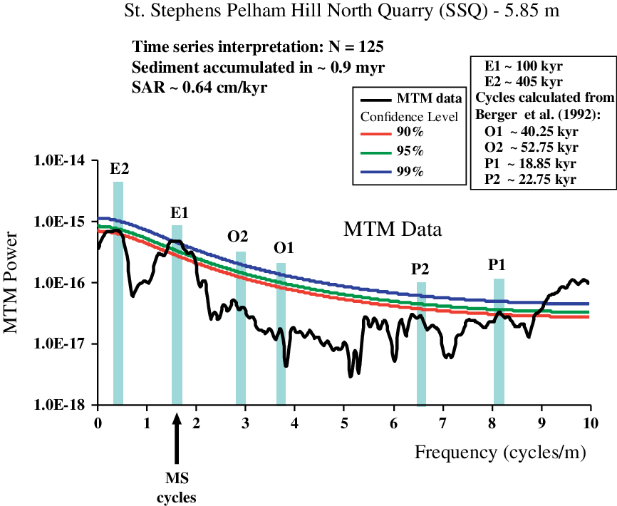
Fig. 15. Time-series analysis (MTM – multi-taper method) of the raw SSQ χ dataset, exhibiting strong E1 (∼100 kyr) and a moderate confidence E2 (∼405 kyr) Milankovitch eccentricity cyclicity. In addition there is a moderate confidence P1 (∼19 kyr) cyclicity. Milankovitch cycles, which were tested for, are given in the upper right corner of the diagram. Sediment accumulation rate (SAR) indicates that the sediment accumulated in ∼0.9 Myr with a SAR of ∼0.64 cm kyr−1.
The approach used was to detrend the raw data, after which the spectral power of the χ data was obtained using the multi-taper method (MTM). Incidences of statistically significant peaks at the 95 and 99% confidence limits in the resulting spectra are determined by employing the MTM (Ghil et al. Reference Ghil, Allen, Dettinger, Ide, Kondrashov, Mann, Robertson, Saunders, Tian, Varadi and Yiou2002), as calculated with the SSA-MTM toolkit (Dettinger et al. Reference Dettinger, Ghil, Strong, Weibel and Yiou1995). A null hypothesis of red noise was assumed (low frequency high power in the spectrum, sloping towards lower values at high frequencies). We limit the use of statistical confidence here to its role in supporting (or not) the positions of multiple Milankovitch bands within the dataset. The positions of these bands are fixed relative to each other, and so a climate forcing mechanism is supported by the spectral analysis when the Milankovitch frequencies are also frequencies of high spectral power. As this approach substitutes space (length along section) for time, non-uniform rates of sedimentation will introduce additional noise into the spectral graph.
The MTM is capable of resolving high-frequency features in the data. Our approach was to (1) collect closely and uniformly spaced samples in the field, (2) report the MTM data, (3) apply confidence limits to the data, and (4) then establish a uniform model using bar-logs that can then be compared to the χ cyclicity as a check on SAR uniformity, or lack thereof. These four elements allow rigorous evaluation of the time-series datasets developed here. The results of this process produced three peaks with high statistical confidence, the strongest being the ∼100 kyr E1 eccentricity peak with confidence level at >99%, followed by the E2 eccentricity at ∼405 kyr, with confidence at ∼95%, and P1 (∼18.9 kyr) precession with confidence levels also at ∼95%. In addition, our analysis of this dataset indicates that the sediment accumulated over a period of ∼0.9 Myr, with an average SAR of ∼0.64 cm kyr−1.
7.a. Timing of SSQ deposition
Timing for the SSQ sequence, which is bracketed by the two unconformities, was calculated based on the high confidence level in the E1 eccentricity time-series data (Fig. 15). These data were then used to graphically correlate the SSQ bar-log distribution to a uniform E1 time scale (Fig. 16). Given that we place the E–O boundary to lie at the conformable Shubuta Clay Member – Red Bluff Formation contact, two different Eocene and Oligocene SARs were calculated from the graphic comparison between a uniform floating point time scale (FPTS) E1 bar-log and the SSQ bar-log that was built from the smoothed χ data (Fig. 9). The result is two relatively well-defined LOC segments (Fig. 16). From these data, the SARs for individual LOC segments were calculated. For the Eocene, the Shubuta Clay Member SAR is ∼0.57 cm kyr−1, while in the Oligocene, the Red Bluff Formation SAR is higher at ∼0.72 cm kyr−1 (Fig. 16). This is consistent with the estimated shallowing versus deepening trends identified in Figure 17 discussed in Section 8 below. In total, the data in Figure 16 represent 50,000 year increments of 100,000 year cycles covering ∼850,000 years through the E–O boundary interval.
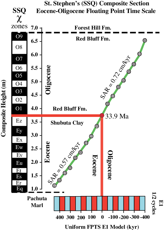
Fig. 16. The SSQ succession from the St Stephens quarry exhibits a relatively well-defined floating point time scale (FPTS) from a time-series analysis of ∼125 samples collected from a ∼6 m succession using raw unsmoothed χ data for the SSQ section bracketed by the two identified disconformities given in Figure 9. χ bar-logs (zones) constructed from the raw χ data (Fig. 9) are graphically compared to a uniform Milankovitch 100,000 year eccentricity climate model (Berger et al. Reference Berger, Loutre and Lasker1992), for the Eocene–Oligocene boundary interval, where each coloured bar represents ∼50,000 years. The intersections of the tops and bottoms of corresponding χ bar-logs and the uniform climate model bar-logs are plotted as stippled dots, and fits through these data are shown as LOC line segments. Using the individual segments, elements from the SSQ section χ bar-logs are projected onto the FPTS and assigned a total length of time of ∼0.9 Myr. This E1 eccentricity climate model provides a FPTS that can be adjusted as timescales change. LOC segments indicate similar sediment accumulation rates (SAR) of ∼0.57 cm kyr−1 in the Shubuta Clay Member and ∼0.72 cm kyr−1 in the Red Bluff Formation, indicating an up-section increase in SAR beginning just before the E–O boundary.
8. Stable isotope (δ18O and δ13C) measurements
8.a. Stable isotopic methods
Carbonate δ13Ccarb and δ18Ocarb were measured using the GasBench II system coupled with a Thermo Finnigan Delta V Advantage isotopic ratio mass spectrometer at the Oxy-Anion Stable Isotope Consortium (OASIC) at LSU. Samples that were analysed were taken from material that had previously been used for magnetic susceptibility measurements, and 1 g of material was chosen from those samples that closely fit the overall lithology of the bed being analysed. Each sample was ground to a fine powder and a ∼0.20 mg split of each sample was weighted for isotopic analysis. Samples were loaded into 12 mL Labco Exetainer vials and sealed with Labco septa that were flushed with 99.999% helium. Samples were then batch acidified by manual injection with ∼100 μL of concentrated phosphoric acid (density = 1.92 g mL−1) at 72 °C. Samples were reacted for 30 minutes prior to the start of sequential isotopic data acquisition. The carbon dioxide analyte gas was isolated via gas chromatography (at 65 °C), and water was removed using a Nafion trap prior to passing through the stable isotope mass spectrometer, which is fitted with a continuous flow interface. Isotopic results are expressed in the delta notation as per mil (‰) deviations from the Vienna Pee Dee Belemnite (V-PDB) standard. The samples were calibrated using an in-house calcite standard (δ18O = −4.31 and δ13C = 2.57). Precision for δ13Ccarb is routinely better than 0.06 ‰, and for δ18Ocarb is routinely better than 0.09 ‰.
8.b. Stable isotopic results
Bulk δ18O and δ13C data were generated for the SSQ succession, and these data are presented in Figure 17. Values for δ18O data show a c. +5 ‰ positive shift (i.e. colder temperatures) below the E–O boundary, which then recover (c. −5 ‰ negative shift) through the boundary interval. Above the boundary these data once again show a slow isotopic enrichment trend suggesting colder temperatures, culminating in another c. +5 ‰ positive shift, reflecting colder temperatures, ∼1.5 m above the boundary. Using the time-series result for the SSQ sequence (Figs 15, 16) this positive shift reaches a maximum ∼250 kyr above the base of the Oligocene. The earlier shift towards a cold climate occurred at ∼300 kyr before the end Eocene extinction event, and may explain the pre-extinction dwarfing in the Hantkeninidae, leading to their extinction.
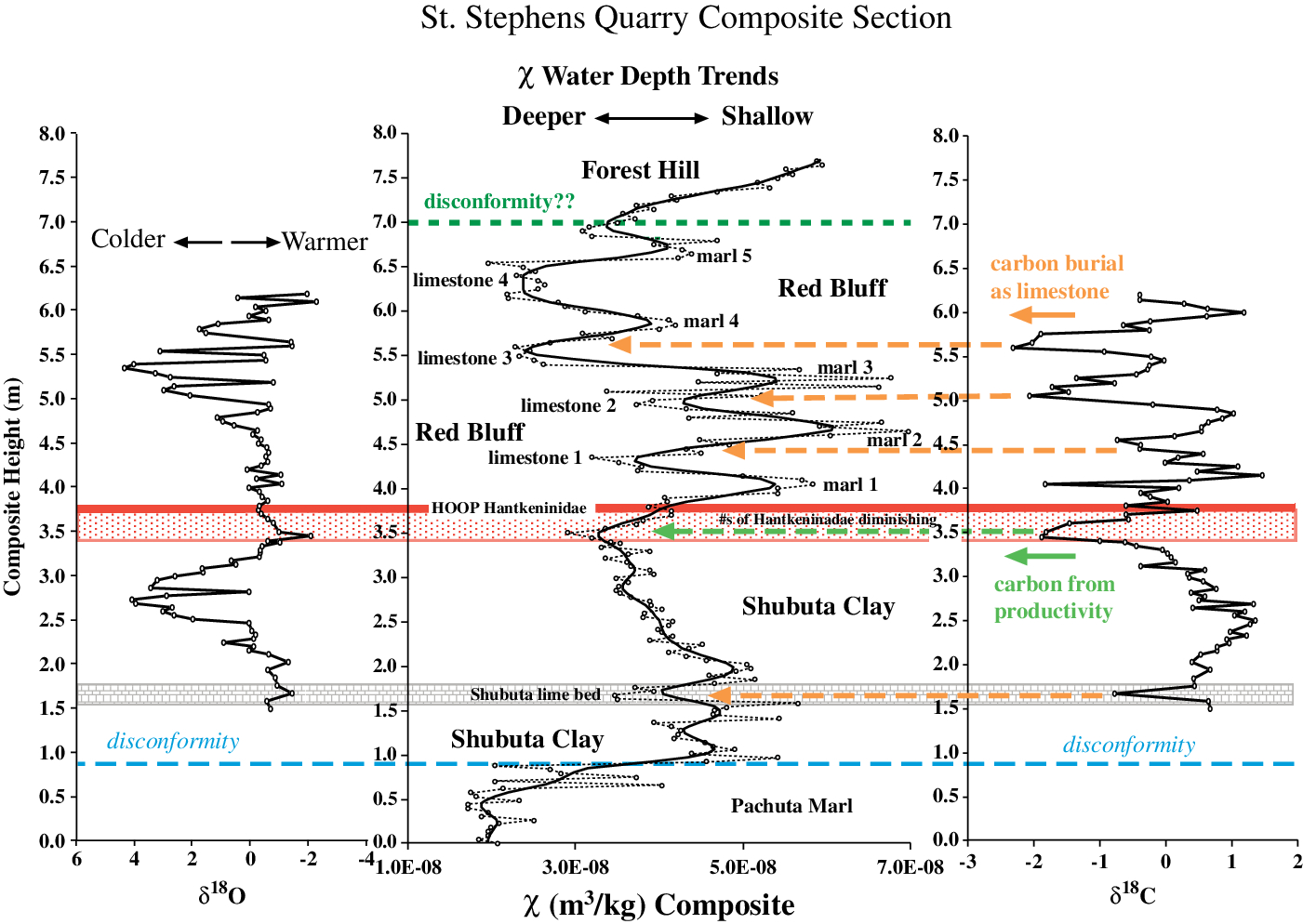
Fig. 17. Oxygen and carbon stable isotopic results from St Stephens quarry compared with the χ trends for the composite section presented in Figure 9. Trends in δ18O are interpreted as ‘colder’ versus ‘warmer’, integrating both ice volume and temperature contributions; χ trends are interpreted as deeper versus shallower based on variations in detrital components controlling the χ trends and on the limestone versus marl deposition; δ13C trends are interpreted in terms of carbon burial as limestone (orange dashed arrows) and carbon burial from productivity (green dashed arrow). Note that the δ13C trends correlate very well with the limestone/marl cycles as represented by lithology and χ trends, and these cycles are visually apparent in the Red Bluff Formation in the St Stephens Quarry (Fig. 5). The stippled zone in the SSQ lies at the top of the conformable transition from the Shubuta Clay Member into the Red Bluff Formation where Hantkeninidae diminish in size and at the top of the zone disappear from the section.
We interpret the δ13C data in the SSQ (Fig. 17) to represent variations in carbon burial as limestone in the Red Bluff Formation, or possibly due to productivity during the pre-extinction dwarfing event at the end of the Eocene, approaching the HOOP of Hantkeninidae. Four distinct limestone beds occur in the Red Bluff Formation in the SSQ, and each of these is marked by a δ13C depletion pulse set that is represented in Figure 17 by dashed light brown arrows. Furthermore, a major c. −3 ‰ negative shift below the boundary appears to correlate with the demise of the larger Hantkeninidae at this locality, after which the gradational zone from Shubuta Clay Member into Red Bluff Formation lithologies begins, as does the pre-extinction dwarfing in the Hantkeninidae. Near the base of the Shubuta Clay Member in the Shubuta lime bed, a c. −3 ‰ negative shift in δ13C occurs.
Results indicate that climate slightly warmed leading up to the E–O boundary, and, just below the boundary, the positive shift in δ18O data are interpreted to indicate cooler sea-surface temperatures. This shift was accompanied by a negative shift in δ13C values, interpreted to indicate the onset of the E–O boundary planktonic foraminiferal extinction event. A second abrupt negative shift in δ18O occurs ∼300 kyr after the E–O boundary and may mark the onset of the Oi-1 glaciation event (Zachos et al. Reference Zachos, Pagani, Sloan, Thomas and Billips2001) that plunged Earth into an icehouse environment. Owing to the large shifts in δ18O of bulk carbonate, it is suggested that a significant portion of the isotopic shift is due to a change in ice volume. For instance, if 90% of the +5 ‰ shift is due to an increase in ice volume, the remaining 10% (0.5 ‰) could reflect a little over ∼2 °C cooling.
9. Conclusions
Six E–O boundary intervals in the SE United States are correlated using a combination of lithostratigraphic, magnetostratigraphic (magnetic susceptibility (χ), geochemical and biostratigraphic methods. The boundary interval is identified using the HOOP of the Hantkeninidae, and these data are supported by changes in other observed foraminifera species. The E–O boundary, identified by the HOOP of Hantkeninidae in SSQ, is placed within the basal marl bed of the Red Bluff Formation of the Vicksburg Group.
In the uppermost Eocene, Hantkeninidae abundance is very low and the size of tests drops due to a pre-extinction dwarfing effect occurring before the final E–O extinctions, with tests becoming difficult to find. This fact may be responsible for some of the uncertainties in picking the E–O boundary at SSQ and elsewhere in the SE United States. χ data at SSQ reflect relatively well-defined, low-magnitude climate cycles during a time of slight climate warming in the uppermost Eocene. This changes to relatively large magnitude cycles in the lowest Oligocene as climate slowly begins to cool, with the effect being that larger pulses of terrigenous grains responsible for χ are being deposited as a component of marine sediment at this time. This observation is supported by an increase in terrigenous palynomorphs, starting at 3.608 m in the SSQ section.
χ and biostratigraphic data allow correlation of the SSQ (western Alabama) to the BQ E–O sections (Florida Panhandle) in the SE United States, and in turn to the E–O GSSP located in central Italy (Jovane et al. Reference Jovane, Sprovieri, Florindo, Acton, Coccioni, Dall’Antonia and Dinarés-Turell2007). All three successions show similar cyclicities. In addition, graphic comparison between the SSQ composite and the GSSP in central Italy shows that estimated residual SARs in both successions were relatively uniform and exhibited relatively uniform cyclicity, although the GSSP SAR in Italy exhibits a significantly higher rate than does the SSQ succession in Alabama.
Author ORCIDs
Brooks Ellwood 0000-0003-2529-9734
Acknowledgements
We are grateful to Prof. Barun Sen Gupta, Sue Ellwood and the many students from the University of Georgia and Louisiana State University who helped with this work over the years; to Mr Jim Long for allowing access to the St Stephens Pelham Hill, North Quarry and for cleaning sections for us using his track-hoe; to Mr Bill Stallworth for allowing us to collect the Red Stuck Quarry; to Mr Leon Brooks for allowing us and our students access to the Marianna Brooks Quarry; and to James Starns and David Dockery of the Mississippi Geological Survey for drilling the Hiwannee Core and discussions in the field. We are also grateful to Amber Ellwood for stable isotopic sample preparation and measurement, and to Huiming Bao and Yongbo Peng for the use of the Oxy-Anion Stable Isotope Consortium (OASIC) laboratory at Louisiana State University. The description of the method used was modified from text provided by Yongbo Peng with his permission. Partial funding for this work came from many sources including the University of Georgia, Louisiana State University and the Robey Clark endowment to the Louisiana State University Department of Geology and Geophysics. Funding was also provided through IGCP Project 652.