


19.1 Introduction
Life’s demand for energy drives rapid exchanges of carbon between the atmosphere, oceans, and land (Reference Regnier, Friedlingstein, Ciais, Mackenzie, Gruber and Janssens1). Photosynthesis and respiration of organic carbon on and near the surface of Earth account for the vast bulk of the transfers of carbon between these reservoirs, processes that dwarf geologic sources and sinks of carbon on short timescales (Reference Mackenzie, Lerman and Andersson2; Chapter 16, this volume). In recent years, however, it has become apparent that Earth hosts a vast subsurface biosphere (Reference Whitman, Coleman and Wiebe3–Reference Balkwill16) that operates much more slowly (Reference Hoehler and Jørgensen17–Reference Jørgensen and Marshall20) than surface life. It is not clear to what depth this biosphere exists, the rates at which it is active, what reactions are being catalyzed for energy, or what impact it has had on Earth’s carbon cycle through time. Extrapolating metabolic rates on Earth’s surface to the subsurface is complicated by an essential difference – the types and rates of biological activity on the surface are determined by daily and seasonal cycles driven by the sun, but life in the subsurface seems to be more attuned to geologic processes and timescales. Such slow rates make it difficult to study subsurface life, but the biological demand for energy can be used to better understand the rates at which these organisms are active and how they interact with their geochemical environments. Studying subsurface life can therefore help reveal the energy limits for life and thus its spatial and temporal extent.
In addition to hosting organisms on the low end of the bioenergetic spectrum, the potential size of the subsurface biosphere motivates many researchers studying deep life. Marine sediments alone have been estimated to contain 1029–1030 microbial cells (Reference Parkes, Cragg, Roussel, Webster, Weightman and Sass4, Reference Kallmeyer, Pockalny, Adhikari, Smith and D’Hondt5) and occupy 300 million km3, over 22% of the volume of Earth’s oceans (Reference LaRowe, Burwicz, Arndt, Dale and Amend21). A similar number of microorganisms are thought to inhabit the continental subsurface (Reference McMahon and Parnell9, Reference Magnabosco, Lin, Dong, Bomberg, Ghiorse and Stan-Lotter22; Chapter 17, this volume). Cells have been found as deep as 3.5 km beneath the surface of land, which, if true of all continental crust, would translate to a potential habitable volume of over 730 million km3 (taking the total continental crust surface to be 2.1 × 10⁸ km2; Reference Cogley23). Although there are no estimates of the size of the ocean crustal basement biosphere, if the top 600 m of it is sufficiently hydrologically permeable to host life (Reference Anderson, Zoback, Hickman and Newmark24–Reference Fisher, Alt, Bach, Stein, Blackman, Inagaki and Larsen32), this would correspond to 1.8 billion km3 (based on the ocean crust covering 68.8% (2.99 × 10⁸ km2) of Earth’s surface; Reference Cogley23). Most recently, it has been estimated that the deep subsurface contains about 13% of the biomass on the planet (Reference Bar-on, Phillips and Milo10). Finally, although we have no information about current or past life on extraterrestrial bodies in our solar system, it is most likely that any evidence of it will be in the subsurface (Reference Jakosky and Shock33–Reference Vance, Harnmeijer, Kimura, Hussmann, Demartin and Brown35).
Cell counts, microbial cultivation work, and molecular biological efforts are helping to describe the numbers, viability, activity levels, and variety of microorganisms in subsurface environments (Chapters 17 and 18, this volume). However, the relative inaccessibility of these environments, the difficulty of cultivating representative microorganisms, and the long timescales associated with some of their lifestyles are major impediments to obtaining a comprehensive understanding of complex subsurface ecosystems. Hence, modeling approaches that include geochemical data as well as typical microbiological measurements can be useful strategies for quantifying biogeochemical interactions in the subsurface. Because all living things must catalyze redox reactions to obtain energy and the amount of energy available from a chemical reaction depends strictly on the prevailing environmental conditions, energy-based modeling provides a framework for quantifying microbial processes in any setting. In this chapter, we will discuss what is known about the microbial demand for energy in low-energy settings, review recent efforts to quantify the energy available in subsurface habitats, and provide an overview of how these calculations are carried out.
19.2 Microbial States
The physiological state of a microorganism is related to the rate at which it is using energy. In contrast to the four classical physiological states that microbial isolates exhibit in high-energy, high-nutrient, short-timespan laboratory experiments – lag, exponential, stationary, and death phases – microorganisms in nature are often nutrient and energy limited and exist in complex communities that are exposed to varying physiochemical properties such as oscillating temperature, pH, and water activity. Their physiological states do not necessarily correspond to those that have been determined in the laboratory and are in many instances unknown (Reference Jørgensen and Marshall20, Reference Bradley, Amend and LaRowe36). Consequently, the rate at which these organisms are processing carbon and energy in nature is not well constrained. Back of the envelope-style calculations reveal how unlikely widespread microbial growth is in nature: if every microorganism in the subsurface (~1030 organisms with ~10 fg C cell–1) doubled every day, all of the carbon in Earth’s crust (60 million Gt; Reference DePaolo37) would become microbial biomass in less than 23 days.
Whatever the physiological status of living microorganisms in natural settings, their use of energy can be partitioned into two broad categories: maintenance and growth. It is difficult to strictly separate maintenance and growth activities because when organisms are growing, they are also carrying out maintenance functions. Similarly, the critical maintenance activity of replacing biomolecules is an aspect of the anabolic processes that lead to growth. Nonetheless, they are commonly viewed as distinct states with particular energetic ramifications.
Maintenance generally refers to the collections of activities that an organism performs to simply stay alive. It can include nutrient uptake, motility, the preservation of charged membranes, excretion of (bio)molecules, and changes in stored nutrient concentrations (see Reference van Bodegom38 for a review). It is difficult to determine the amounts of energy that each of these and other maintenance functions require, so they are typically lumped together and defined in the negative: all of the activities that a microorganism carries out that are not associated with growth. Traditionally, maintenance energies are determined by growing microorganisms at ever-slower rates and extrapolating the amount of energy that they use to a value that would represent zero growth (for a review, see Reference Hoehler and Jørgensen17). Values reported in the literature range over more than five orders of magnitude, from 0.019 fW (fW ≡ femtowatts, 10–15 J s–1) for anoxygenic phototrophy to 4700 fW for aerobic heterotrophy (see Reference LaRowe and Amend39). This procedure might decipher the energy partitioned into nongrowth activities for a high-energy state – growth – but maintenance energies in nature are orders of magnitude lower than these values (Reference Hoehler and Jørgensen17, Reference Lever, Rogers, Lloyd, Overmann, Schink and Thauer18, Reference LaRowe and Amend39–Reference LaRowe and Amend41).
To distinguish laboratory measurements of maintenance from the survival state of microorganisms in nongrowing and other low-energy environments, the term “basal power requirement” has been introduced (Reference Hoehler and Jørgensen17). The use of the word “power” instead of “energy” is apt (see Reference LaRowe and Amend39, Reference LaRowe and Amend41, Reference Shock and Holland42) since so-called maintenance energies are given in units of energy per time. Recent results from modeling studies support the notion that in very-low-energy settings (e.g. deep oligotrophic marine sediments such as those under the South Pacific Gyre), maintenance powers are indeed several orders of magnitude lower than those reported in the literature, from 50 to 3500 zW cell–1 (where zW ≡ zeptowatt, 10–21 W; Reference LaRowe and Amend41). Related calculations suggest that the amount of particulate organic matter required to sustain microbes at a basal power level in the same oligotrophic environment is equivalent to about 2% of their biomass carbon per year (Reference Bradley, Amend and LaRowe36). It should be noted that these latter two studies assume that all of the energy used by these microbes is for maintenance only, not growth. It is not known whether microorganisms in ultra-low-power settings produce daughter cells or merely persist via maintenance (Reference Hoehler and Jørgensen17, Reference Lever, Rogers, Lloyd, Overmann, Schink and Thauer18, Reference Jørgensen and Marshall20). It is thought that very slow or no growth is the norm in many environments (Reference Morita43), especially chemically stagnant, low-energy ones such as oligotrophic marine sediments (Reference Hoehler and Jørgensen17, Reference D’Hondt, Spivack, Pockalny, Ferdelman, Fischer and Kallmeyer44–Reference Røy, Kallmeyer, Adhikari, Pockalny, Jørgensen and D’Hondt46). However, it should be noted that when conditions improve, metabolic rates can increase dramatically (Reference Morono, Terada, Nishizawa, Ito, Hillion and Takahata47). Although values are not well constrained for dynamic ecosystems, maintenance power can vary due to many factors, including temperature (for the same species), substrate identity, redox conditions, and cultivation techniques (Reference Lever, Rogers, Lloyd, Overmann, Schink and Thauer18).
Microbial growth can refer to the generation of new cells, the production of biomass accompanying enlarging cells and the synthesis of external structures such as stalks, sheaths, tubes, biofilms, and other polymeric saccharides. Although extracellular biomass can be a significant fraction of the total biomass of a system, most efforts to quantify the amount of energy that it takes to make biomass have focused on the energetics of making cells, and like all chemical reactions, the amount of energy required to synthesize cells depends in large part upon the physiochemical properties of the environment. The first modern effort to explicitly quantify how environmental parameters influence the energetics of biomass synthesis focused on how the redox state of the environment influences the energy required to synthesize the biomolecules that make up cells (Reference McCollom and Amend48). More recently, LaRowe and Amend (Reference LaRowe and Amend49) expanded this analysis to quantify the amount of energy required to make biomass as a function of temperature, pressure, redox state, the sources of C, N, and S, and cell mass, while also accounting for the polymerization of monomers into biomacromolecules such as proteins, DNA, RNA, and polysaccharides (see below). These kinds of modeling results depend on both the compositions and the masses of microbial cells. The stoichiometry of biomass varies considerably (see Reference Lever, Rogers, Lloyd, Overmann, Schink and Thauer18, Reference LaRowe and Amend49 for reviews), with the average nominal oxidation state of carbon (NOSC; see 50) in cell biomass – a tidy numerical representation of the ratio of carbon to hydrogen, nitrogen, oxygen, sulfur, and phosphorous in organic matter – varying from at least from +0.89 to –0.45 (Reference LaRowe and Amend49). Note that the commonly used stand-in for biomass, “CH2O,” fixes the NOSC at 0. As with maintenance power, cell stoichiometry varies with environmental conditions (see 49).
Other attempts to account for the energy required to make biomass rely upon laboratory experiments that are designed to promote growth, conditions that are rarely encountered in the subsurface (see Reference LaRowe and Amend39 for a review). In addition, numerous energy-based models developed to predict biomass yields have limited applicability because they are restricted to standard and/or reference states (for reviews, see Reference LaRowe and Amend39, Reference Heijnen and van Dijken51). Most of these models fix biomass yield coefficients, which leads to predictions of equal biomass production (for the same synthesis reactions) under potentially very different environmental conditions. Other efforts seeking to determine the amount of energy required to make biomass rely on estimates of the number of moles of ATP that are required to carry out various aspects of biomolecular synthesis. A commonly cited version of this approach (Reference Russell and Cook52) reports the ATP requirements for various anabolic and maintenance functions. The reference for these values ultimately cites a paper (Reference Stouthamer53) that effectively assumes the amount of ATP required for a variety of biochemical processes with little to no experimental evidence or references. Even if the amount of ATP required to synthesize biomass were well constrained in natural settings, the amount of energy that is released from the hydrolysis of ATP to ADP and phosphate is a function of the physiochemical characteristics of the environment in which it is happening, and therefore not a constant (Reference LaRowe and Helgeson54–Reference LaRowe and Helgeson56).
Microorganisms can also enter into low-energy and dormant states. While some authors use the term “dormancy” to describe low-energy states as well (Reference Lennon and Jones57), others reserve this term for true endospore-forming microorganisms that are metabolically inactive (Reference Nicholson, Munakata, Horneck, Melosh and Setlow58). Sensu stricto, dormancy is a reversible, contingent state that is entered into when resources become limiting. Because there is no metabolic activity, critical functions such as DNA and protein repair are not possible. As a result of abiotic hydrolysis, oxidation, and other degradative processes, dormant organisms have a finite lifespan. Although little is known about the energetics or maximum possible length of dormancy (Reference Lever, Rogers, Lloyd, Overmann, Schink and Thauer18, Reference Morita43), there is evidence that revival rates are inversely correlated with the amount of time a microorganism spends in the dormant state (Reference Morita43, Reference Kaprelyants, Gottschal and Kell59), an observation that has been included in modeling studies of microbial dormancy (Reference Stolpovsky, Fetzer, Van Cappellen and Thullner60, Reference Stolpovsky, Martinez-Lavanchy, Heipieper, Van Cappellen and Thullner61). One study showed that the number of endospores in frozen samples decreases with sample age since endospores do not have active DNA-repair mechanisms, but that low-energy bacteria in the same samples can survive for up to half a million years (Reference Johnson, Hebsgaard, Christensen, Mastepanov, Nielsen and Munch62).
Microorganisms in low-energy states, in contrast to dormant ones, are able to slowly metabolize in order to remain viable for potentially millions of years (Reference D’Hondt, Inagaki, Zarikian, Abrams, Dubois and Engelhardt19, Reference Jørgensen40). These low-energy states are thought to be prevalent in natural systems, to exist on a spectrum of levels, and to have multiple entry points (Reference Lennon and Jones57). In fact, it is possible that <10% of microbial cells in soil and aquatic environments are active (Reference Locey63). One estimate proclaimed that low-energy cells can exist on three orders of magnitude lower power than typical maintenance power levels (Reference Price and Sowers64), though, as pointed out above, maintenance powers determined under relatively high-energy conditions span five orders of magnitude. Perhaps energy usage in the low-energy state is more akin to basal maintenance power as defined by Hoehler and Jørgensen (Reference Hoehler and Jørgensen17): the flux of energy required for a minimum survival state. Some speculate that virtually all microbial cells in deep marine sediments are surviving in ultra-low energy states (Reference Jørgensen and Marshall20). A recent modeling study represented the cells in an oligotrophic marine sediment section as existing in a series of ever-lower energy states, but none as truly dormant (Reference Bradley, Amend and LaRowe36).
19.3 Gibbs Energy: Where It Comes from and How to Use It
All organisms catalyze reactions as they acquire energy from the environment and carry out biochemical functions related to maintenance and growth. The amount of energy associated with these chemical transformations depends on the exact identity of the reaction – all of the reactants and products describing the mass- and charge-balanced process – as well as the prevailing temperature, pressure, and composition of the environment in which it is happening. The mathematical approach that is used to quantify the change in energy resulting from a chemical reaction is the Gibbs function, denoted by G. Despite being well known, it is worth noting why this, of several energy functions related to the internal energy of a system, is the one that is used to assess how energy is required by organisms to perform a given task and how much energy results from catalyzing reactions that ultimately fuel life’s demands. For textbook-level overviews of thermodynamics, see (Reference Kondepudi and Prigogine65–Reference Garrels and Christ68).
Because there is no absolute energy scale, we can only discuss changes in the amount of energy that a system contains. The change in the internal energy (U) of a system can be quantified by assessing changes in the temperature (T), pressure (P), volume (V), and entropy (S) of it, quantities that can be modified by the exchange of heat and matter between the system and the surroundings as well as reactions happening within the system. Changes in the internal energy of the system, dU, can be mathematically linked to how these four variables change in different ways (i.e. the various energy functions are effectively different partial derivatives of U with respect to T, P, V, and S). These four variables are known as state variable because they describe the state of the system at any given moment; functions including these variables are known as state functions. For instance, the change in the amount of heat (or enthalpy, H) associated with a system at constant pressure, dHP, with no chemical reactions occurring, can be defined by dHP = dU + PdV, which is a simple statement of the first law of thermodynamics – the conservation of energy (technically, this and other state functions hold for infinitesimal changes taking place in the time interval t to t + dt). Enthalpy is a useful state function that describes the evolution of the heat content of a system, but it cannot predict how the system will evolve. The Gibbs energy function accomplishes this by combining the first law of thermodynamics with the second law, which essentially states that the entropy of an isolated system cannot decrease (see Box 19.1).
Entropy is sometimes wrongly discussed in terms of being equivalent to “disorder.” This confusion likely arises from Boltzmann’s statistical mechanical interpretation of entropy being related to the number of microstates that a system can occupy – the more microstates, the higher the entropy. The proliferation of the use of the word “entropy” in other fields (e.g. Shannon entropy in information theory, which is more akin to uncertainty than the classical definition of entropy as a quantity of energy) has contributed to the popular conception of entropy as a measure of disorder. From its origins with Carnot and developments by Clausius, de Donder, and Kelvin, entropy is described as a quantity of energy and a state variable; its units are J K–1 mol–1. The classical definition of entropy is that it is equal to the change in the heat of a system, Q, at a given temperature: dS = dQ/T.
Prigogine and Defay (69) describe two ways in which the entropy of a system can change: (1) entropy can be transported across the boundary of a system and therefore be positive or negative; and (2) entropy can be generated inside of an isolated system due to the occurrence of chemical reactions – these reactions are irreversible and the net change of entropy associated with them is always positive, dS > 0. It is this inequality that ultimately specifies the direction in which a system will evolve. So, we can say that the entropy of a system changes due to entropy exchanges with the surroundings (dSe) and entropy created within the system, dSi, or dS = dSe + dSi. Because dSi is related to the degree to which chemical reactions are occurring, it is in turn related to the extent to which a reaction has occurred. The extent of a reaction is known as ξ, and sometimes is called the reaction progress variable (Reference Prigogine and Defay69–Reference de Donder71). Changes in the reaction progress variable for a reaction are related to the stoichiometric coefficients of the ith species in that reaction, vi, by
 (19.a)
where ni refers to the number of moles of the ith species produced or consumed in the reaction. For example, the extent to which the reaction describing hydrogen-consuming sulfate reduction,
 (19.b)
has progressed, dξ(19.b), is given by
 (19.c)
Clearly, when dni = vi, dξ(19.b) = 1 and the reaction is said to have turned over.
The reaction progress variable and entropy are connected through what is known as chemical affinity, A, a term that is sometimes used to quantify how far a system is from equilibrium: dSi = Adξ ≥ 0 (this equation is also known as de Donder’s fundamental inequality and can be thought of as another statement of the second law of thermodynamics). Although chemical affinity and the Gibbs energy of a reaction are related simply by A = –ΔGr, the two quantities have important conceptual differences. A is defined as the change in Gibbs energy resulting from changes in the reaction progress variable while pressure, temperature, and composition (nk) are held constant (Reference de Donder and Van Rysselberghe70, Reference de Donder71):
 (19.d)
As such, affinity relates irreversible chemical reactions to entropy production, while the Gibbs energy of a reaction is traditionally used in reference to equilibrium states and reversible processes (see Reference Anderson and Crerar66). Furthermore, chemical affinity can be connected to reaction rate as a measure of the distance that reaction is from equilibrium (Reference Prigogine and Defay69, Reference de Donder and Van Rysselberghe70, Reference van’t Hoff72, Reference Aagard and Helgeson73).
Within this conceptualization, thermodynamic rate-limiting terms have been developed in kinetic models that relate the rates of biologically catalyzed reactions to their distance from equilibrium, with reactions closer to equilibrium being slower than those further away (Reference Jin and Bethke74–78). Finally, affinity and the rate of entropy production have in turn been used to develop more recent developments in the field of nonequilibrium thermodynamics, especially systems far from equilibrium and the establishment of dissipative structures, such as life (see Reference Kondepudi and Prigogine65).
Changes in the Gibbs energy at constant temperature and pressure are commonly expressed as dGT,P = dH – TdS, or in integrated form, ΔG = ΔH – TΔS, but is more clearly linked to changes in the internal energy state of a system by dGP,T = dU + PdV – TdS. By incorporating the second law of thermodynamics, the Gibbs energy function quantifies the tendency of a chemical reaction to proceed in a particular direction. That is, for a given chemical reaction, negative values of ΔG indicate that if a reaction occurs, the net result is the formation of products at the expense of reactants; the opposite direction occurs for positive values of ΔG. When ΔG = 0, there is no net reaction and equilibrium has been reached.
Thus far, we have represented thermodynamics functions with simple letters like G and H. However, if we want to use these functions to calculate the energetics of real processes under specific environmental conditions, we must become familiar with the alphabet soup of subscripts and superscripts that modify and specify the meanings of terms such as G and H. As noted above, since we can only know how the energy of a system changes, the upper case Greek letter delta, Δ, is often placed in front of energy functions to signify changes in values of that function (e.g. ΔG and ΔH). These should be thought of in terms of the difference in, for example, the Gibbs energy of the system at one configuration versus another: ΔG = G2 – G1. How the system evolved from state 1 to state 2 is irrelevant. When the subscript r is added, ΔGr, for example, stands for the Gibbs energy of a reaction. These subscripts are straightforward accoutrements decorating thermodynamics functions, but the superscripts are less so, and they are typically more meaningful. When the superscript 0 appears, (i.e. ΔG0), the symbol is explicitly referring to the change in Gibbs energy at a standard state. Standard states are one of the most frequently misunderstood aspects of thermodynamics.
The standard state used in traditional chemical thermodynamics does not refer to a temperature or pressure (i.e. it does not refer to 25°C and 1 bar), but a standard state of aggregation, or composition (see Figure 19.1 for a conceptual overview). The reason for this is that, as discussed above, we cannot know the internal energy, U, of a system, but we can determine changes in it. Both Gibbs energies and enthalpies are partial derivatives of U, so to quantify ΔG0, ΔH0, and other such standard state terms, we need a coherent system that relates the thermodynamic functions describing compounds to a set of standards. The system that is used in chemical thermodynamics to define the Gibbs energies and enthalpies of chemical compounds is related to that of the elements. For example, the standard-state Gibbs energy of formation from the elements of gaseous methane,  , is calculated based on the change of Gibbs energy associated with the reaction:
or:
 (19.2)
where  and
and  refer to the standard-state Gibbs energies of formation for elemental carbon as graphite and gaseous dihydrogen, respectively, and
  denotes the standard-state Gibbs energy of (19.1). These compounds are chosen because they are the stable phases of these two elements at the reference conditions of 25°C and 1 bar. The phase and form of the standard-state Gibbs energies and enthalpies of most elements are defined as those that are stable at 25°C and 1 bar, and they are all taken to be zero only at this temperature and pressure – their values are not zero at other combinations of temperature and pressure.
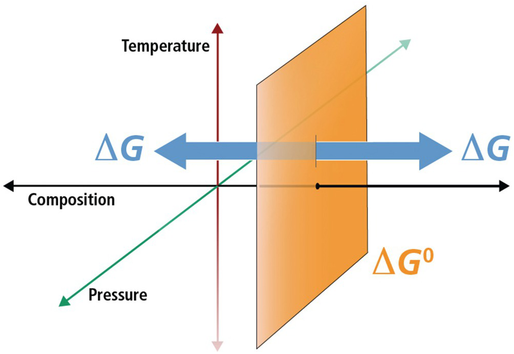
Figure 19.1 Schematic diagram illustrating the difference between standard-state Gibbs energies ( ) and overall Gibbs energies (ΔGr) in temperature, pressure, and compositional space. For a given standard state, values of
  refer to a fixed composition at any combination of temperatures and pressures (the orange plane) and that departures from this composition are what distinguish ΔGr. For gases, pressure is part of the standard-state definition since the state of aggregation of a gas is partially determined by its partial pressure.
Staying with the CH4 example, since the values of  and
and  are 0 J mol–1 at 25°C and 1 bar and the value of
  for (19.1) is –50.4 kJ mol–1, then
  = –50.4 kJ mol–1 at 25°C and 1 bar (the value of
  is determined from a series of calorimetric measurements that are beyond the scope of this chapter). At any other combination of temperature and pressure, values of
  and
and  are not 0 J mol–1 and therefore the value of
  does not equal that of
  (see Figure 19.2). For instance, at 300°C and 86 bars, they are –2.8 and –38.8 kJ mol–1, respectively, and
  for (19.1) is –25.24 J mol–1. Therefore,
  = –105.6 kJ mol–1 at 300°C and 86 bars, more than twice the value at 25°C and 1 bar. Beyond stipulating that the forms of the elements that are used in calculating the Gibbs energies of formation are their stable ones at 25°C and 1 bar, temperature and pressure are not part of the definition of standard-state properties for substances, except for the standard state for gases (see below). Although this is a rather tedious discussion, it is presented to illustrate how temperature and pressure are properly taken into account in thermodynamic calculations, which are particularly important for quantifying the energetics of biogeochemical processes in the subsurface.

Figure 19.2 Standard-state Gibbs energies (ΔG0) of H2 gas, carbon as graphite, CH4 gas, and the reaction defining the formation of methane from the elements as a function of temperature (see (19.1) and (19.2)). The vertical dashed lines at 25°C and 300°C are marked in reference to the examples discussed in the text.
In addition to specifying that the definition of the chemical standard state relates thermodynamic properties of chemical species to those of the elements at particular combinations of temperature and pressure, it also specifies the state of aggregation of chemical substances. The commonly used standard state of aggregation differs depending on the phase, and to be accurate, the amount of a substance that is used to define standard states is activity, rather than concentration (discussed below). Similarly, amounts of gases are represented by fugacities instead of partial pressures. The standard state of gases is that of unit fugacity of the pure hypothetical ideal gas at 1 bar and any temperature, that of liquids and solids is unit activity of the pure substance at any temperature or pressure, and that of aqueous species is unit activity in a hypothetical 1 molal solution referenced to infinite dilution at any temperature and pressure. This last one is a bit peculiar owing to its impossibility, but it is necessary since the concentration, and thus the distances between dissolved chemical species, can vary by many orders of magnitude in natural systems on and near Earth’s surface. Furthermore, since aqueous species are dissolved in a medium that has its own thermodynamic properties, such as water, the interactions between the solvent and dissolved species must also be accounted for in any standard state of aggregation (see Box 19.2).
Box 19.2 G0 as a function of temperature and pressure and the equilibrium constant.
Many texts incorrectly state that the definition of standard state for all phases specifies a pressure of 1 bar (e.g. Reference Kondepudi and Prigogine65). However, a cursory glance at the equation that describes how values of the standard-state Gibbs energy of a system or substance at any temperature and pressure,  , differ from that at the reference temperature of 25°C and pressure of 1 bar,
 , quickly shows why this is wrong for all phases other than gases:
 (19.e)
where  refers to the standard molal entropy of the species at the reference pressure and temperature,
  stands for the isobaric molal heat capacity at the reference pressure, and V0 designates the standard molal volume. The fourth term on the right-hand side shows how standard-state Gibbs energy changes as a function of pressure when temperature is held constant,
  . Adding the provision that 1 bar is part of the standard state for solids, liquids, and aqueous species would neglect the volume integral in (19.e) and thus its contribution to the standard-state Gibbs energy. The equilibrium between graphite and diamond further illustrates this point.
The simplified carbon phase diagram presented in Box Figure 1 shows the combinations of temperature and pressure at which graphite and diamond are in equilibrium; that is,  = 0 for
That is, the standard-state Gibbs energies of graphite and diamond are equal on this line. Another way to look at this is to use the more intuitive, and aptly named, equilibrium constant, K. The value of K for (19.f) is 1 for the temperatures and pressures that define the curve in Box Figure 1. Values of K are related to the standard-state Gibbs energy via:
 (19.g)
Again, if a pressure of 1 bar were set for the standard-state values of  for graphite and diamond, it would be impossible to account for the impact of pressure on the equilibrium state between graphite and diamond. In fact, there would be no stability field for diamond without elevated pressure, no matter the temperature.
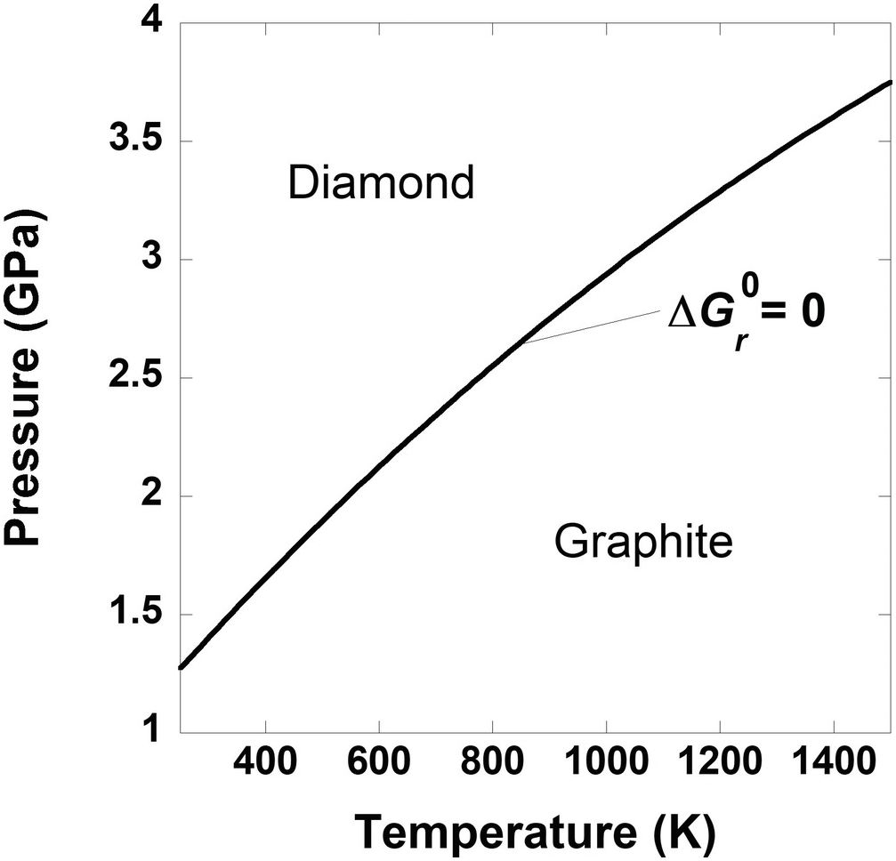
Box Figure 1 A phase diagram for carbon. The curve represents the set of temperatures and pressures where graphite and diamond are in equilibrium,  = 0.
= 0.
For the interested reader, the first three terms on the right-hand side of (19.e) result from taking into account that both enthalpy and entropy are integrals of  and thus represent how these thermodynamic functions vary with temperature at constant pressure:
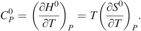 (19.h)
If one knows how  varies with temperature, then
  can be calculated for temperatures and pressures other than 25°C and 1 bar. This is rather straightforward for many liquids, gases, and solids; the widely used Maier–Kelley formulation for
  is used:
  . Regression of experimental calorimetry data and/or estimation schemes can be used to determine species-specific values of a, b, and c. However, in the aqueous state, expressions for
  and V0 as a function of temperature – and pressure – are more complex due to the interactions of aqueous species with the solvent. The revised Helgeson–Kirkham–Flowers (HKF) equations of state are commonly used to calculate the standard-state thermodynamics properties of aqueous species at temperatures and pressures other than 25°C and 1 bar (see Reference Tanger and Helgeson79–Reference Helgeson, Kirkham and Flowers85). The requisite thermodynamic data and equation-of-state parameters for using this model for thousands of aqueous species have been published in the literature (see 50 for a summary of organic compounds, Reference Helgeson, Delany, Nesbitt and Bird86 for a summary of minerals, and Reference Sverjensky, Shock and Helgeson87 for inorganic aqueous species, among many others). The SUPCRT92 software package (Reference Johnson, Oelkers and Helgeson80) is commonly used to calculate standard-state thermodynamics properties of species as a function of temperature and pressure using the revised HKF model. In the R language and computing environment, CHNOSZ has many of the capabilities of SUPCRT92, as well as a variety of plotting and other functions (Reference Dick88: chnosz.net).
In many biological applications, the so-called biochemical standard state is used, a term that is typically not rigorously defined (see 56, Reference Amend and Shock89, Reference Canovas and Shock90). The Interunion Commission on Biothermodynamics (Reference Wadsö, Gutfreund, Privalov, Edsall, Jencks and Armstrong91) recommends that the biochemical standard state should correspond to pH = 7, and the temperature should be 25°C or 37°C, the ionic strength should be set by a 0.1 M KCl solution, concentrations can be used in place of activities, and the concentrations of a group of similar species can be added together and treated as one species (i.e. [ATP] = [ATP4–] + [HATP3–] + [H2ATP2–] + [MgATP2–] …). Although it is relatively straightforward to convert thermodynamic data reported in the biochemical standard state to the traditional chemical standard state for pH and ionic strength, using it is complicated by the fact that the exact version of the biochemical standard state being used is often not specified (i.e. which of the recommendations noted above are being followed). For instance, one of the most widely cited papers on the thermodynamics of chemical reactions in the biochemical literature (Reference Thauer, Jungermann and Decker92) defines a biological standard state similar to one by the Interunion Commission on Biothermodynamics, but also reports so-called observed Gibbs energies that, in addition to fulfilling the biochemical standard state, also sets the ionic strength to 0.25 and a free Mg2+ concentration to 0.001 M. Another problem with the biochemical standard state is that some of the researchers who use it and want to expand it report values of standard Gibbs energies of formation from the elements,  , for some species to be zero simply because they do not have thermodynamic data for them (see Reference Canovas and Shock90). Clearly, this violates the basis of Gibbs energies and enthalpies being based on the Gibbs energy of formation from the elements, which are 0 in their respective reference states at 25°C and 1 bar. This introduces enormous errors that cannot be corrected like pH and ionic strength can be. In addition, many of those who use the biological standard state to compute Gibbs energies of processes rarely use the reaction quotient term, Q, which takes into account composition of the solution, the impact of which is seen in the example calculations presented below. Furthermore, it is worth pointing out that pH 7 only defines solution neutrality (aH+ = aOH−) at 25°C and 1 bar in pure water. Neutral pH at 37°C is 6.81, and at 150°C and 5 bars it is 5.82 (pH = − log aH+). Finally, if the preceding paragraphs have failed to demystify what standard states are, simply remember that they are about purity (composition) and the elements, and that they are only part of calculating the Gibbs energy of a reaction.
The Gibbs energy of a chemical reaction, ΔGr, is a function of temperature, pressure, and the composition of the system – not just the activities of the reactants and products of the reaction of interest, but also the concentrations of all of the other chemical species in the system:
 (19.3)
where R represents the gas constant and T denotes temperature in Kelvin (see Figure 19.1). The standard-state Gibbs energy of reaction,  , is simply equal to the difference in the standard-state Gibbs energies of the products and reactants in a reaction, both multiplied by their respective stoichiometric coefficients, νi:
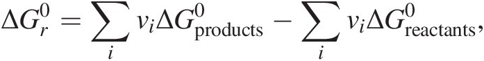 (19.4)
as shown in (19.2) above for reaction (19.1). The reaction quotient, Qr, a frequently neglected term, is essential to quantifying the Gibbs energy of any reaction that an organism is catalyzing to gain energy. It is responsible for bringing compositional reality into the accurate computation of ΔGr and is calculated as the product of the activities of the reactants and products, ai, in a chemical reaction raised to their stoichiometric coefficients, νi:
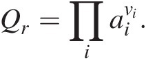 (19.5)
Evaluating (19.3)–(19.5) requires that a mass- and charge-balanced reaction has been written to represent a process, and therefore that the identities of all of the product species are known. In some cases, this becomes difficult to ascertain since many common biological elements, such as C, N, and S, have many oxidation states and therefore many different ways to balance the transformation of these elements.
As an example, Qr for the sulfate reduction shown in Box 19.1, reaction (19.b) is
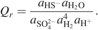 (19.6)
If only standard-state values of Gibbs energies were used to calculate ΔGr for (19.b), the resulting calculation would only be valid for activities of all of the species in this reaction being 1 (see Section 19.4 for examples). Since these activities are set by the standard state, it would be equivalent to having 1 molal concentrations of each species in an infinitely dilute solution – an impossible situation. Imagine an environment in which the concentration of all five of these species is 1 molal. At 25°C and 1 bar, this would be a pH of 0 and far beyond the solubility of H2. Ignoring the Q term when calculating the Gibbs energies of chemical reactions is effectively ignoring physical reality. Using only standard electrical potentials (E0) to calculate the energetics of reactions is similarly untethered from physical possibilities (see Reference Amend and Teske93).
The way that nonideal conditions (i.e. nonstandard states) are quantified is to use activities in place of concentrations and fugacities instead of partial pressures of gases when evaluating the Qr term. The concepts of fugacity and activity were developed to account for thermodynamic deviations between ideal and observed behavior (see Reference Lewis and Randall94). By close analogy, the ideal gas law only describes the relationship between the amount, temperature, pressure, and volume of a gas (nRT = PV) within certain limits of these parameters. When a gas is very concentrated, this simplistic law breaks down and requires additional terms to describe the relationships among the variables in it. Similarly, activity and fugacity account for the nonideal behavior of substances when they are under relatively high concentrations and/or exposed to temperatures and pressures that are far beyond their reference temperatures and pressures. They can be thought of as the effective thermodynamic concentrations of liquids, solids, gases, and aqueous species.
Values of activity are calculated from the concentration of a substance, C, and its activity coefficient, γ: a = Cγ (a more accurate representation of this relationship is a = γ(C/C0), where C0 stands for a substance’s concentration in the standard state – activity and activity coefficients do not have units). There is a vast and complex literature on how to measure and compute values of γ (e.g. see Reference Anderson and Crerar66, Reference Helgeson and Kirkham83, Reference Helgeson, Kirkham and Flowers85, Reference Pytkowicz95), but suffice to say that they are typically calculated rather than measured for a particular set of conditions. A commonly used model to calculate activities for aqueous species that incorporates elevated temperatures, pressures, and ionic strengths is the extended version of the Debye–Hückel equation (Reference Helgeson96). Software such as Geochemist’s Workbench (www.gwb.com) and PHREEQC (www.usgs.gov/software/phreeqc) is commonly used to compute activities, as well as to carry out speciation calculations.
Related to the concept of activity is that of speciation. In solution, a given chemical species, especially charged ones, is partitioned among a variety of forms. For instance, in seawater, total sulfate concentration is about 28 mM, and though sulfate exists primarily as  at 18.1 mM, the remainder of it is complexed with cations commonly found in seawater. Abundant complexes include
  (7.6 mM),
  (6.2 mM),
  (0.8 mM), and
  (0.2 mm). Any calculation of Qr should take such speciation into account, as well as the activity coefficient of
  , which in seawater at 25°C and 1 bar is 0.16. Thus, the activity of
  in seawater at 25°C and 1 bar is 0.0029, nearly an order of magnitude lower than its total concentration of 0.028 M.
Analogous to activity, fugacity (f) is the thermodynamic equivalent of pressure, taking into account the differences between the mechanical pressure exerted by a gas (P) and its effective pressure: f = Pχ, where f takes on units of pressure such as bars and the fugacity coefficient, χ, is unitless (see Reference Appelo, Parkhurst and Post97).
19.4 Temperature, Pressure, and Composition Affecting G
The amount by which variable temperature, pressure, and composition affect the Gibbs energies of chemical reactions can vary tremendously (see Reference Amend and Shock89). Although a number of studies have appeared in the literature demonstrating how different combinations of these variables impact reaction energetics (discussed below), the impact that each of these variables can have alone, and in various combinations, is demonstrated here by using the low-energy metabolism known as hydrogenotrophic acetogenesis:
The curves in Figure 19.3a show the values of  from 0°C to 150°C and the values of ΔGr for the same reaction under different compositional conditions that characterize high- and low-energy states (the activities of CO2, H2, and CH3COO– and pH are taken to be 10–3, 10–8, and 10–4 and 5 for the low-energy case and 10–1.3, 10–3, and 10–8.5 and 9 for the high-energy scenario, respectively). For reference, the diamond shape in Figure 19.3a shows the Gibbs energy of (19.7) under conditions corresponding to the biological standard state,
  , which is more exergonic than even the high-energy scenario, so perhaps it is not very relevant to natural systems. Although the values of
  , the traditional chemical standard-state Gibbs energy, fall between those of the high- and low-energy scenarios, they are much closer to the high-energy state. Notably, ΔGr for the low-energy case is endergonic throughout the temperature range considered here. Therefore, if one were to use standard-state values of Gibbs energies to quantify how much energy acetogens are gaining by catalyzing (19.7) – at any temperature – when the chemical composition of the system was that specified for the low-energy case, then the direction of the reaction would be wrong: fermentation of acetate (the reverse of (19.7)) would be predicted rather than acetogenesis. Most natural environments could be described by compositions between the high- and low-energy scenarios described here and therefore have values of ΔGr between the two lines representing them.
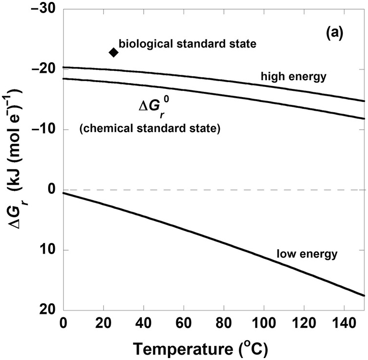
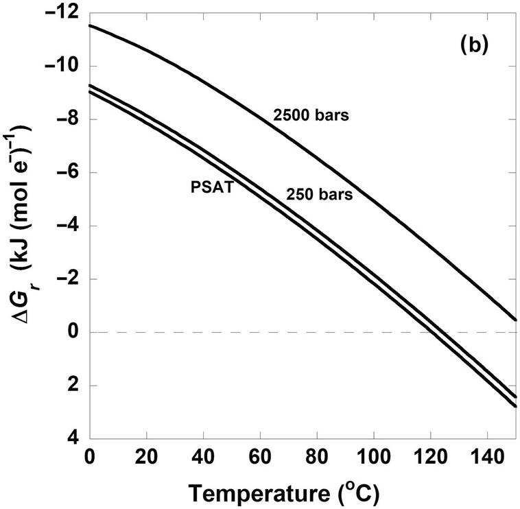
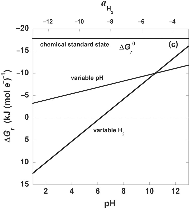
Figure 19.3 Gibbs energies of hydrogenotrophic acetogenesis, 2CO2(aq) + 4H2(aq) → CH3COO– + H+ + 2H2O, as a function of (a) temperature for the biological and traditional chemical standard states as well as low- and high-energy scenarios, (b) temperature and pressure, and (c) pH and activity of hydrogen, aH2.
The quantitative impact of different pressures on (19.7) is shown in Figure 19.3b. Here, each curve represents ΔGr of this reaction for activities of CO2, H2, and CH3COO– and pH equal to 10–1.7, 10–3, and 10–6 and 7, respectively, at saturation pressure (PSAT – just enough pressure to keep water liquid), 250 bars, and 2500 bars. It is clear that values of ΔGr do not differ much between PSAT and 250 bars, and that the difference between PSAT and 2500 bars is just over 2 kJ (mol e–)–1. This is a general feature of the quantitative impact of pressure on the Gibbs energies of catabolic reactions. It should be noted that this only takes into account pressure differences on  for (19.7) and that pressure can have large effects on the solubility of gases such as CO2 and H2, which can lead to higher activities of these compounds at the high pressures often found in the subsurface. These pressure effects on activities would be represented in the Qr term.
For many microbial processes, the most important variable effecting values of ΔGr is the Qr term, or, in other words, the composition of the system. This can clearly be seen in Figure 19.3c, where ΔGr for (19.7) is shown as a function of pH and H2 activity, while temperature, pressure, and the activities of the other constituents of (19.7) are held constant (25°C, 1 bar, activities of CO2 and CH3COO– are 10–1.7 and 10–6; for variable pH, aH2= 10–6 and for variable aH2, pH = 7). For reference,  for this reaction is shown at 25°C and 1 bar and is a flat line at –17 kJ (mol e–)–1. Note that both ranges of aH2 and pH result in much less exergonic values of ΔGr than would be calculated by using standard-state values. What is apparent from the stoichiometry of (19.7) and Figure 19.3c is that for every order of magnitude change in aH2, there is a much larger change in ΔGr than for each integer change in pH. In fact, the acetogenesis pathway represented by (19.7) is no longer thermodynamically favored at pH 7 once aH2 falls below about 10–8.5. As a sidenote, the steep dependence of ΔGr on pH shown in Figure 19.3c is typically even more exaggerated in reactions describing the oxidation and reduction of iron, with added variability depending on which iron minerals are involved in the reaction (see Reference Rowe, Yoshimura, LaRowe, Bird, Amend and Hashimoto98).
19.5 Surveying Gibbs Energies in Natural Systems
Because microorganisms have evolved the ability to catalyze a wide variety of redox reactions to gain energy under a broad set of physiochemical conditions, there are usually multiple catabolic strategies capable of sustaining a given ecosystem, particularly in subsurface environments that light does not reach. As a result, many of the studies that have quantified the Gibbs energies or chemical affinities (see Box 19.1) of plausible energy-sustaining reactions in subsurface settings have examined a large set of potential catabolic reactions: the thermodynamic potentials of hundreds of chemical reactions have been reported for submarine hydrothermal systems (Reference Amend, McCollom, Hentscher and Bach99–Reference Dahle, Økland, Thorseth, Pedersen and Steen109), shallow-sea hydrothermal systems (Reference Price, LaRowe, Italiano, Savov, Pichler and Amend110–Reference Lu, LaRowe, Gilhooly, Druschel, Fike and Amend117), terrestrial hydrothermal systems (Reference Inskeep, Ackerman, Taylor, Kozubal, Korf and Macur118–Reference Costa, Navarro, Shock, Zhang, Soukup and Hedlund124), marine sediments (Reference LaRowe, Dale and Regnier125–Reference Schrum, Spivack, Kastner and D’Hondt132), the terrestrial subsurface (Reference Osburn, LaRowe, Momper and Amend133–Reference Kirk, Jin and Haller135), serpentinizing systems (Reference Canovas, Hoehler and Shock136), specific-element systems such as arsenic (Reference Amend, Saltikov, Lu and Hernandez137), the ocean basement (Reference Edwards, Bach and McCollom138–Reference Boettger, Lin, Cowen, Hentscher and Amend141), and even extraterrestrial settings (Reference Shock142–Reference Marlow, LaRowe, Ehlman, Amend and Orphan145). The majority of these studies focus on chemolithotrophic catabolic strategies because concentrations of specific organic compounds are not commonly reported (for exceptions, see Reference Rogers and Amend112, Reference LaRowe and Amend146–Reference Lever, Heuer, Morono, Masui, Schmidt and Alperin148). In fact, the pairs of electron donors and acceptors that are considered are typically those whose concentrations have been measured, which tends not only to narrow the list of metabolisms considered, but also to establish a somewhat consistent set of metabolic redox pairs that are evaluated for their catabolic potential.
The Gibbs energies reported in the studies mentioned above range from endergonic (ΔGr > 0) to nearly –160 kJ (mol e–)–1. The amount of energy available from a given reaction varies considerably between study sites and even within them. For example, Shock et al. (Reference Shock, Holland, Meyer-Dombard, Amend, Osburn and Fischer120) calculated values of ΔGr for ~300 reactions using temperature, pressure, and compositional data from dozens of hot springs in Yellowstone National Park, USA. Their results showed that the Gibbs energies for nearly 15% of the reactions that they considered could be exergonic or endergonic, mostly depending on the composition of the individual hot spring fluids. In a similar study, Lu (Reference Lu149) examined the thermodynamic potential of 740 potential catabolic reactions along a two-dimensional transect in sediments next to a shallow-sea hydrothermal vent and found that 559 are exergonic in at least one location.
Although the large number of reactions considered in these and related studies can seem overwhelming, there are a handful of salient points that can be distilled from them beyond the obvious one that many different metabolisms are possible in any given ecosystem. One observation is that the thermodynamic favorability of reactions involving common powerful oxidants such as O2 and NO3– are not necessarily the most exergonic reactions in some environments: the oxidation of Mn2+ by O2, for instance, can easily be endergonic, while the oxidation of CO by NO2– (to CO2 and N2) can yield more energy than any reaction involving O2 (Reference Lu149). Composition tends to have a much bigger impact on the energetics of metabolic reactions than either temperature or pressure. The pH of a fluid is responsible for large differences in the values of ΔGr for the same reaction, especially for those involving iron (Reference Shock, Holland, Meyer-Dombard, Amend, Osburn and Fischer120, Reference LaRowe, Amend, Kallmeyer and Wagner127, Reference Kirk, Jin and Haller135). The wide range of Gibbs energies available from a given electron acceptor shows that the identity of it is not sufficient to predict the order of electron acceptors used by microorganisms (Reference Bethke, Sanford, Kirk, Jin and Flynn150), a well-known hypothesis in marine science that asserts that organisms in sediments use terminal electron acceptors in the order of their energetic potential (Reference Claypool, Kaplan and Kaplan151–Reference Stumm and Morgan153) – an idea that is ultimately based on standard-state Gibbs energies of reaction and restricted to the oxidation of fermentation products. Finally, it is worth pointing out that quantifying the potential energetic landscape in difficult-to-access subsurface environments can be used to predict where novel catabolic reactions could be happening. This is similar to how both the anaerobic oxidation of methane by sulfate and anaerobic ammonium oxidation were predicted based on the thermodynamic calculations demonstrating the Gibbs energies of these reactions (Reference Reeburgh154, Reference Broda155).
As noted above, Gibbs energy calculations aimed at revealing metabolic potential and involving organic carbon are relatively rare, or are restricted to a small number of compounds such as acetate and other volatile organic acids (e.g. Reference Rogers and Amend112, Reference Windman, Zolotova, Schwandner and Shock123, Reference LaRowe, Dale and Regnier125, Reference Glombitza, Jaussi and Røy130, Reference Kirk, Jin and Haller135, Reference Lever147, Reference Lever, Heuer, Morono, Masui, Schmidt and Alperin148). This is certainly an improvement over the common treatment of representing organic carbon as “CH2O” and thus having a fixed energetic potential that is typically tied to the Gibbs energy of glucose. This is a convenient way of not dealing with the complexity of naturally occurring organic matter – a vast mixture of compounds that vary in their size, charge, oxidation state, structure, and composition. As an extreme example, it is worth noting that Kevlar (polyparaphenylene terephthalamide) and ethanol are both forms of organic matter, yet their properties are wildly divergent.
Although identifying organic compounds in the subsurface is difficult, characterization techniques are improving (Reference LaRowe, Koch, Robador, Witt, Ksionzek and Amend156–Reference Shah Walter, Jaekel, Osterholz, Fisher, Huber and Pearson159), and the thermodynamic properties of thousands of organic compounds have been reported in the literature (see 50 for a review, and, for more recent studies, see Reference Canovas and Shock90, Reference LaRowe and Amend146, Reference LaRowe and Dick160). Even if organic compounds cannot be identified, if the average NOSC in them can be, then the standard-state Gibbs energy of oxidation can be estimated (Reference LaRowe and Van Cappellen50); the range of  for the half-oxidation reactions for organic compounds varies by at least 23 kJ (mol e–)–1 (Reference LaRowe and Van Cappellen50). The reactivity of organic carbon in the subsurface would certainly be better understood if the thermodynamic properties of more organic compounds were known.
19.6 Energy Density
Although a thermodynamic calculation can be useful for determining whether a certain reaction is favored to occur under particular environmental conditions, it does not reveal any information about whether the reaction occurs or at what rates, and therefore how many organisms could be supported by it. Ideally, concentration gradients, rate measurements, and/or modeling tools should be used in conjunction with Gibbs energy calculations (e.g. Reference LaRowe, Dale, Aguilera, L’Heureux, Amend and Regnier106, Reference Jin and Bethke134, Reference Dale, Regnier and Van Cappellen161–Reference André, Pauwels, Dictor, Parmentier and Azaroual167) to quantify which reactions are driving the biogeochemistry of a system. However, even in the absence of kinetic information, Gibbs energies of reaction can be scaled to units that reveal information about ecosystems that would be otherwise obscured.
Many of the studies noted in Section 19.5 report the Gibbs energies or affinities of potential catabolic reactions in units of kJ mol–1 or kJ (mol e–)–1. The latter provides a common basis on which to compare the potential of many redox reactions, though this tends to leave out disproportionation and comproportionation reactions. However, both energy-per-mole units can give a very misleading view of what are the most energy-yielding reactions in an environment. Reactions involving oxygen as the oxidant are especially relevant. For example, ΔGr for the oxidation of glucose to CO2 by O2 is –117 kJ (mol e–)–1 (for logaO2 = − 4, logaCO2 = − 1.7, logaglucose = − 4, and logaH2O = 0 at 25°C and 1 bar). Keeping the activities of everything else constant and lowering the activity of O2 by ten orders of magnitude (logaO2 = − 14) results in ΔGr = –103 kJ (mol e–)–1, only a 12% change (logaO2 would have to be lowered to –86.4 to make this reaction endergonic; for reference, this would be equivalent to about 1000 molecules of O2 in a volume of water equivalent to the volume of the Milky Way). Even if a concentration of O2 corresponding to logaO2 = − 14 could be measured, any environment characterized with this amount of oxygen would be considered anoxic. Yet, a straightforward thermodynamic calculation shows that it is very exergonic, implying that it should be a likely metabolic activity in the environment. If one presents the results of the same calculations in terms of energy densities (e.g. Reference McCollom103, Reference LaRowe, Amend, Kallmeyer and Wagner127), then about 0.01 kJ (kg H2O)–1 would be available in the high-O2 case and 10–12 J (kg H2O)–1 in the latter, if all of the O2 could be used instantaneously (typically, energy densities are calculated by multiplying the concentration of the limiting reactant in a reaction by its Gibbs energy, taking into account the stoichiometry of the reactants).
On the low end of the energy spectrum, ΔGr of glucose oxidation by sulfate, for example, is –21 kJ (mol e–)–1 (for logaHS− = − 5, pH = 8, logaCO2 = − 1.7, logaglucose = − 4, logaH2O = 0, and  at 25°C and 1 bar), which is about one-fifth of ΔGr for the analogous reaction with O2 as the oxidant – when the activity of O2 is 10–14. The energy density of the sulfate reaction is nearly 0.6 kJ (kg H2O)–1, more than even the high-O2 activity calculations. Interpreting these results is not straightforward: on a molar or per-electron basis, O2 yields far more energy than sulfate, no matter what the activity of O2 is, but the energy density of sulfate plus glucose is greater than that of the analogous high-O2 scenario. One would not expect sulfate reduction to be a prominent glucose oxidation pathway when oxygen is abundant, but it certainly makes sense that sulfate reduction is a more dominant glucose oxidation pathway when oxygen concentrations are below what is currently measurable. Clearly, some combination of common sense and other data will be useful for interpreting the meaning of thermodynamic calculations of catabolic potential, regardless of what units are used.
The units that have been reported for the Gibbs energy calculations summarized above tend to correlate with the environmental system being examined. For example, values of ΔGr in deep-sea hydrothermal systems tend to be reported in units of J (kg H2O)–1 because these calculations are based on the in silico mixing of different masses of fluids that drastically differ in temperature and composition. With different ratios of hydrothermal fluid to seawater and highly variable concentrations of electron donors and acceptors in hydrothermal fluid, the Gibbs energies available for a given reaction from mixing fluids can vary by many orders of magnitude in these units. Typically, the most exergonic reactions for a particular ratio of hydrothermal fluid to seawater are the ones that are reported in these studies: H2S, CH4, H2, and Fe2+ oxidation can provide more than 1000 J/kg H2O (Reference Amend, McCollom, Hentscher and Bach99), and H2 oxidation can provide up to 3700 J /kg H2O when hydrothermal fluids from ultramafic systems mix with seawater (Reference McCollom100). However, under unfavorable mixing ratios, the amount of energy available from some potential catabolic reactions, such as Fe2+ and H2S oxidation, can be four to eight orders of magnitude lower than the most optimal conditions (Reference Houghton and Seyfried104).
The practice of reporting both molal Gibbs energies of potential catabolic reactions and energy densities for some systems (e.g. shallow-sea hydrothermal, marine sediment, and terrestrial systems) is growing (e.g. Reference Price, LaRowe, Italiano, Savov, Pichler and Amend110, Reference Teske, Callaghan and LaRowe126, Reference LaRowe, Amend, Kallmeyer and Wagner127, Reference Osburn, LaRowe, Momper and Amend133, Reference Lu149). These studies all show very different results when Gibbs energies are reported in both molal and density units. For instance, LaRowe and Amend (Reference LaRowe, Amend, Kallmeyer and Wagner127) compared the Gibbs energies of 18 reactions in three marine sedimentary environments characterized by different physiochemical conditions, varying mostly in composition. They showed that when values of ΔGr were normalized by the concentration of the limiting reactant (i.e. Gibbs energies were presented as energy densities), the order of the most energy-rich reactions changed considerably and the energy available from different reactions varied by about six orders of magnitude per cm3 of sediment. Furthermore, they showed that trends in cell abundance as a function of depth do not follow the most exergonic reaction – per mole of substrate – but by those with the highest energy densities.
A global overview of Gibbs energy densities of chemolithotrophic metabolisms in terrestrial hot springs, shallow-sea hydrothermal systems (<200 m water depth), and deep-sea hydrothermal systems is shown in Figure 19.4. The Gibbs energies of potential catabolic reactions consisting of different combinations of 19 electron acceptors and 14 electron donors were evaluated for 326 data sets describing the geochemistry of 30 distinct systems. Of the 740 reactions considered, 571 are exergonic at one or more sites. The reactions are ordered from the most exergonic to the least based on the Gibbs energies per electron transferred. Because the compositions of deep-sea hydrothermal systems are often reported as those of calculated end-member hydrothermal fluids, which are typically too hot for life, the results shown in Figure 19.4c were generated by computing the energy densities of this end-member hydrothermal fluid mixed with enough seawater such that the resulting fluid was 72°C, equal to the mean temperature for the terrestrial hot springs and shallow-sea hydrothermal systems represented in the other two panels in Figure 19.4 (see Reference Lu149 for details). It can be seen that for many of these reactions, the amount of energy available from a particular combination of electron donors and acceptors varies by many orders of magnitude, reflecting the compositional diversity of global hydrothermal systems. Furthermore, these energy densities span nearly 12 orders of magnitude. The reactions in deep-sea systems tend to have higher energy densities and the reactions in shallow-sea systems tend to show broader ranges. Although there is a sigmoidal pattern for ordering the Gibbs energies of these reactions per electron transferred (see Reference Lu149), there is no such pattern here. This is because when Gibbs energies are presented in energy density units, directly accounting for the concentration of the limiting electron donor or acceptor, the order of which reaction is most energy yielding can change dramatically.

Figure 19.4 Global overview of Gibbs energy densities of chemolithotrophic metabolisms in (a) terrestrial hot springs, (b) shallow-sea hydrothermal systems (<200 m water depth), and (c) deep-sea hydrothermal systems. The Gibbs energies of potential catabolic reactions consisting of different combination of 19 electron acceptors and 14 electron donors were evaluated for 326 data sets describing the geochemistry of 30 distinct systems. The horizontal bars represent the ranges of energy densities for a given reaction and the dots refer to the average energy density of that reaction. Of the 740 reactions considered, 571 are exergonic at one or more sites. The reactions are ordered from the most exergonic to the least based on the Gibbs energies per electron transferred (not shown). Because the compositions of deep-sea hydrothermal systems are often reported as those of calculated end-member hydrothermal fluids, which are typically too hot for life, the results shown in (c) were generated by computing the energy densities of this end-member hydrothermal fluid mixed with enough seawater such that the resulting fluid was 72°C. See (Reference Lu149) for details.
19.7 Time
Time plays a number of roles in determining the energy limits for life. On a fundamental level, active organisms must be able to catalyze redox reactions faster than they are catalyzed abiotically if they are to gain energy from them. This observation has been more colorfully expressed as “things that burst into flame are not good to eat” (Reference Shock and Boyd168). Iron oxidation is one such potential metabolism. Although the oxidation of FeReference Mackenzie, Lerman and Andersson2+ with O2 is a very exergonic reaction under most environmental conditions, the abiotic rate of this process is so fast under certain combinations of pH and temperature that organisms cannot take advantage of the disequilibria. This has been shown to be the case in samples taken from lakes and springs in Switzerland (no biological catalysis for pH >7.4) and hot springs in Yellowstone National Park (no biological catalysis for pH > 4.0, at elevated temperatures) (Reference St. Clair169). Similarly, sulfide oxidation can proceed so quickly in hyperthermophilic settings that isolates capable of catalyzing this reaction, such as Thermocrinis ruber, cannot gain energy from it (Reference Härtig, Lohmayer, Kolb, Horn, Inskeep and Planer-Friedrich170).
Microorganisms that are not competing with the abiotic catalysis of potential catabolic reactions still must use energy to combat the slow, abiotic decay of biomolecules such as the depurination of nucleic acids and the racemization of amino acids (Reference Lever, Rogers, Lloyd, Overmann, Schink and Thauer18, Reference Jørgensen and Marshall20), reactions that accelerate as temperature increases (Reference Price and Sowers64, Reference Steen, Jørgensen and Lomstein171). These most basic functions are part of what is known as basal maintenance functions, the absolute minimum flux of energy required to keep a cell viable. Because the rates of biomolecular repair likely approach that at which they are needed, it is difficult to determine the lowest amount of power on which a microorganism can survive. However, marine sediments, with their potential to record environmental data over geologic timescales, can serve as natural laboratories to constrain the basal power limits for life. Geochemical data, cell counts, and modeling efforts have been combined to estimate that microorganisms living in sediments under the South Pacific Gyre are metabolizing organic carbon with oxygen mostly at 50–3350 zW (Reference LaRowe and Amend41). In the same study, the authors hypothesize that an organism could survive on as little at 1 zW.
It is worth clarifying that the lower power limits for life should not be confused with mechanistic arguments that have been made regarding microbial activity and energy minima (see Reference Harder172). Essentially, it has been proposed that microorganisms require a minimum amount of Gibbs energy from a catabolic reaction (Reference Jin and Bethke75, Reference Schink173–Reference Hoehler175) that is significantly less than ΔGr < 0. Models that make use of this essentially stipulate that once the Gibbs energy of a particular catabolic reaction dips beneath a given minimum, microorganisms can no longer catalyze the reaction to gain energy (see Reference LaRowe, Dale, Amend and Van Cappellen78 for an overview). A lower microbial power limit, on the other hand, is simply a flux of energy large enough to keep the cell viable.
19.8 The Cost of Anabolism
As noted above, it is difficult to decipher how microorganisms partition the energy that they get from the environment. However, no matter what state microorganisms are in – growing, maintaining, or some low-level form of dormancy – they must make and/or repair biomolecules to exist for extended periods of time. The identities and quantities of these biomolecules are not well known, nor is the rate at which they must be replaced. What we can determine is the amount of energy associated with the reactions that describe biomolecule synthesis under the temperature, pressure, and compositional conditions prevailing in the deep biosphere. Efforts to do this fall into two groups: (1) those that have sought to determine whether particular organic compounds and biomolecules are thermodynamically favored to be abiotically synthesized under, typically, hydrothermal conditions; and (2) those that quantify the amount of energy required to build the biomolecules that constitute a cell under a variety of environmental conditions (for a review, see Reference Amend, LaRowe, McCollom and Shock176). Falling into the first group, calculations have shown that the abiotic formation of alkanes, alkenes, alcohols, ketones, aldehydes, carboxylic acids, amino acids, nucleic acid bases, and monosaccharides can be favored to form when particular hydrothermal fluids mix with seawater and kinetic barriers are assumed to prevent carbon transformations to CO2 or CH4 (Reference Amend and Shock177–Reference LaRowe and Regnier181).
The second group of studies focused on the energetics of organic synthesis and quantified the amount of energy that is required to build most of the biomolecules that constitute a cell in the proportions that exist in a model microorganism, Escherichia coli (Reference Battley182). McCollom and Amend (Reference McCollom and Amend48) calculated the Gibbs energy required to make all of the biomonomers that make a cell, starting from inorganic precursor molecules (HCO3– (NH4+ and NO3–), HPO4Reference Mackenzie, Lerman and Andersson2– (H2S and SO4Reference Mackenzie, Lerman and Andersson2–)) under microoxic and anoxic oxidation states. The cost of making biomonomers was 13–15 times higher in the microoxic environment than the anoxic one, depending on the sources of N and S. In an extension of this study, LaRowe and Amend (Reference LaRowe and Amend49) assessed the amount of energy associated with making the same set of biomolecules, but also quantified the role of pressure and used a wider range of redox conditions, temperatures, sources of C, N, and S, and cell sizes. Taken together, environmental variables – and the range of cell sizes – lead to an approximately four orders of magnitude difference between the number of microbial cells that can be made from a Joule of Gibbs energy under the most (5 × 10¹¹ cells J–1) and least (5 × 10Reference Edwards, Wheat and Sylvan7 cells J–1) ideal conditions.
Finally, a few authors have published calculations in which they have quantified the amount of energy that it takes to synthesize microbial biomass due to the disequilibria resulting from mixing seawater with hydrothermal fluids of variable composition. Amend and McCollom (Reference Amend, McCollom, Zaikowski, Friedrich and Seidel183) focused on the early Earth, while Amend et al. (Reference Amend, McCollom, Hentscher and Bach99) analyzed how hydrothermal fluids whose compositions were influenced by different water–rock interactions impacted the energetics of biomass synthesis. They showed that the most energetically favorable temperatures were between 22°C and 32°C in general, and that hydrothermal fluids that interacted with peridotite and troctolite–basalt hybrid rock systems created the most favorable energetic conditions for producing biomass, yielding up to 900 J per g dry cell mass.
19.9 Concluding Remarks
What combination of natural variables defines the limits to life? The discovery of abundant life in the subsurface has expanded this search to: How deep life can exist? How long can it maintain itself under nearly isolated conditions? And what is the minimum power that it can get by on? One way to address these questions is to determine where and when microorganisms no longer get energy as fast as they need it. In the deep subsurface, this threshold will likely be defined by the power required to repair biomolecules. Essential biomolecules such as nucleotides, amino acids, saccharides, and lipids all undergo abiotic decay through a variety of reactions, including racemization, methylation, deamination, isomerization, radiation exposure, and hydrolysis, while biomacromolecules like DNA, RNA, and proteins can become cross-linked and/or unfolded. The rates of all of these processes depend on the environmental context, particularly temperature. Repairing biomolecules requires energy, and the acquisition of energy requires the maintenance of membrane potentials and the ability to transport nutrients and energy substrates across membranes. Although the energetics and rates of amino acid racemization and DNA depurination have received a fair amount of attention (Reference Lever, Rogers, Lloyd, Overmann, Schink and Thauer18), it is not known how all of these degradative processes are influenced by the various combinations of physiochemical and temporal extremes that often define subsurface settings. Identifying the biotic fringe in the subsurface will require quantification of how temperature, pressure, and chemical composition impact the rates of biomolecular decay and how much power is available to rectify this decomposition.
Although we do not always have the information needed to evaluate the amount of catabolic power that is used deep below the surface, we often have the requisite information to quantify the Gibbs energy that is available for microbial energy demands as well as the cost of making biomolecules in situ. In this chapter, we have reviewed how temperature, pressure, and composition affect the Gibbs energies of chemical reactions associated with staying alive in the deep biosphere and how to accurately quantify it. We have belabored the point that the traditional chemical standard state refers to the composition of a system and not temperature and pressure (except for gases), and that the chemical composition of an environment is typically much more significant for calculating the Gibbs energy of a catabolic or anabolic reaction than temperature and pressure. The examples provided illustrate that there is no cheap shortcut to quantifying how much energy is associated with a given chemical reaction under specified physiochemical conditions and that care must be taken to interpret the results of these calculations: Gibbs energies are potentials that can be used to quantify the direction of natural processes and are therefore useful for constraining what life is possible of doing in the subsurface or in any environment.
Acknowledgments
We appreciate the comments provided by anonymous reviewers. This work was supported by the NSF-sponsored Center for Dark Energy Biosphere Investigations (C-DEBI) under grant OCE0939564; the NASA Astrobiology Institute – Life Underground (NAI-LU) grant NNA13AA92A; the USC Zumberge Fund Individual Grant; the NASA-NSF Origins of Life Ideas Lab program under grant NNN13D466T; and the Alfred P. Sloan Foundation through the Deep Carbon Observatory. This is C-DEBI contribution 453 and NAI-LU contribution 134.
Questions for the Classroom
1 Why does the usage of Gibbs energies and other thermodynamic properties require standard states?
2 What are the limitations of the biochemical standard state?
3 What are the factors influencing the amount of energy an organism gains by catalyzing redox reactions?
4 What is the advantage of using chemical affinities rather than overall Gibbs energies of reactions to quantify the tendency of a chemical reaction to proceed?
5 What is the utility of reporting the results of Gibbs energy calculations in density rather than molar units? What are the shortcomings?
6 How does the redox state of an environment influence the amount of energy that is required to make biomass?
7 Why does one need to know the identities and concentrations of products in a catabolic reaction to quantify the amount of energy an organism gains from it?
8 Use the CHNOSZ software package (chnosz.net) to calculate how different fugacities (partial pressures) of CO2 impact the Gibbs energies of acetoclastic and hydrogenotrophic methanogenesis. Hint – see the vignette on chemical affinity on the CHNOSZ website.
9 Calculate how different fugacities of H2 impact the Gibbs energies of hydrogenotrophic methanogenesis.


 Open access