


1. Introduction
The interaction between surface water waves and underlying currents affects the wave properties significantly (Longuet-Higgins & Stewart Reference Longuet-Higgins and Stewart1961), as also confirmed by experiments, e.g. Swan, Cummins & James (Reference Swan, Cummins and James2001). The interaction is hence of practical interest for design of offshore structures; see recent comparisons of structural responses with and without this interaction considered (Chen & Basu Reference Chen and Basu2018a,Reference Chen and Basub) where linear wave–current interaction models were used, however; for coastal engineering applications (Kirby & Dalrymple Reference Kirby and Dalrymple1983; Dong & Kirby Reference Dong and Kirby2012) and in geophysical fluid dynamics (Kirby Reference Kirby1984; Kirby & Chen Reference Kirby and Chen1989). Of most interest is the problem of two-dimensional (2-D) periodic water waves propagating on a steady current. A large number of theoretical studies and numerical investigations have been dedicated to this problem. However, it is still far from being fully understood. A comprehensive introduction to nonlinear wave–current interactions can be found in Constantin (Reference Constantin2011).
In fact, it is only recently that the existence of the large-amplitude wave solutions for rotational flows with general vorticity (thus allowing arbitrary current profiles) in finite water depth has been proved by Constantin & Strauss (Reference Constantin and Strauss2004). Prior to this, only waves of small amplitude were known to exist in the presence of vorticity (Dubreil-Jacotin Reference Dubreil-Jacotin1934). Hur (Reference Hur2006) further extended the proof of Constantin & Strauss (Reference Constantin and Strauss2004) to the case of infinite depth with the additional restriction that the vorticity distribution is positive and monotone. Hur (Reference Hur2011) later completed the proof of existence of large-amplitude waves with infinite depth removing the mentioned restrictions on vorticity. Moreover, Constantin & Strauss (Reference Constantin and Strauss2011) and Strauss (Reference Strauss2012) addressed the existence of periodic travelling waves of small and large amplitude in a flow with an arbitrary bounded but discontinuous vorticity.
Following the work by Constantin & Strauss (Reference Constantin and Strauss2004), rotational flows with constant and non-constant vorticity have received considerable attention. Notably, many numerical investigations, on both irrotational and rotational flows, appeared much earlier. For example, for irrotational flow in finite water depth, Chappelear (Reference Chappelear1961) expanded the velocity field and the wave profile in Fourier series and the Fourier coefficients were numerically determined from the Bernoulli equation by using the least squares method. The direct numerical simulation results were compared with the fifth-order Stokes theory. Dalrymple (Reference Dalrymple1974a) presented a numerical model for steady water waves propagating over a linear-shear current (constant vorticity) where the streamfunction was expressed as the superposition of a linearly varying current profile and an irrotational wave field. The results thereof showed that the vorticity has a significant impact on the wave height. Simmen & Saffman (Reference Simmen and Saffman1985) and Teles da Silva & Peregrine (Reference Teles da Silva and Peregrine1988) studied periodic steady water waves with constant vorticity for infinite and finite water depth, respectively. The numerical methods for irrotational flows and rotational flows with constant vorticity are generally based on the boundary integral method or the Fourier expansion. Recently, Clamond & Dutykh (Reference Clamond and Dutykh2018) developed a novel conformal mapping method for irrotational flows, where the governing equation is rendered of Babenko kind which is then solved using the Petviashvili method. The model is very efficient and is able to solve for large-amplitude waves with quite large steepnesses over arbitrary depth. Dyachenko & Hur (Reference Dyachenko and Hur2019b) further modified the Babenko equation to permit constant vorticity and applied Newton–GMRES (generalized minimal residual) method following the use of the Fourier expansion. There are also other methods that have been developed. For instance, Ablowitz, Fokas & Musslimani (Reference Ablowitz, Fokas and Musslimani2006) proposed a non-local formulation which was further applied to consider non-flat bottom and moving non-flat bottom boundaries (Fokas & Nachbin Reference Fokas and Nachbin2012; Francius & Kharif Reference Francius and Kharif2017). Wahlén (Reference Wahlén2009) and Ehrnström, Escher & Wahlén (Reference Ehrnström, Escher and Wahlén2011) devised a novel transform for small-amplitude waves with constant and linear vorticity, i.e. a vertical scaling transformation.
For waves on rotational flows with non-constant vorticity, early numerical investigations date back to Dalrymple (Reference Dalrymple1973, Reference Dalrymple1977), where the author considered the effects of various current profiles on the finite-amplitude steady waves over finite water depth. The method was based on the Dubreil-Jacotin (DJ) transformation and finite difference discretization of the transformed rectangular domain. For a given boundary condition, the solution to internal points is improved by a number of sweeps; the error on the free-surface boundary condition is then evaluated; subsequently, the solution on the free boundary is updated and the procedure is repeated until convergence. Using this method, Dalrymple & Cox (Reference Dalrymple and Cox1976) showed the influence of the vorticity on wavelength and crest elevation of the wave, considering that the currents vary as trigonometric and hyperbolic sine and cosine functions of the depth. Thomas (Reference Thomas1990) performed experimental studies for a finite-amplitude wave train interacting with a steady current containing an arbitrary distribution of vorticity, and moderate agreement was found between the measurements and the results obtained using the model of Dalrymple (Reference Dalrymple1977). Ko & Strauss (Reference Ko and Strauss2008b) presented a numerical continuation method to find large-amplitude 2-D periodic steady water waves with arbitrary vorticity, which was used for discussing the relationship between amplitude, hydraulic head, depth and mass flux for variable vorticity cases (Ko & Strauss Reference Ko and Strauss2008a). This method neither uses truncated Fourier expansion nor makes any assumption on the water depth or wave amplitude. Further numerical analyses of water waves on rotational flows with discontinuous vorticity can be found in Strauss (Reference Strauss2010), Constantin & Strauss (Reference Constantin and Strauss2011) and Constantin (Reference Constantin2012a). The ethos of the approaches towards wave computation is that the local bifurcation from a laminar flow to a small-amplitude wave solution is predicted by a dispersion relation, the algorithm beginning with the linearized solution. The wave solution is then continued with increasing wave height until the solution becomes close to a wave in a flow with stagnation point (global bifurcation). The dispersion relation has been derived for small-amplitude periodic water waves travelling on rotational flows for various vorticity cases, e.g. see Constantin & Strauss (Reference Constantin and Strauss2011) and Constantin (Reference Constantin2012a) and Martin (Reference Martin2015) for flows with two layers. Karageorgis (Reference Karageorgis2012) discussed dispersion relations for several types of non-constant vorticities. High-order approximations for the constant vorticity case were discussed in Constantin, Kalimeris & Scherzer (Reference Constantin, Kalimeris and Scherzer2015a). Amann & Kalimeris (Reference Amann and Kalimeris2018) expanded upon the method of Ko & Strauss (Reference Ko and Strauss2008b), by allowing non-uniform grid points and enabling the continuation with vorticity as a bifurcation parameter. Using the latter scheme they successfully discovered a new part of the bifurcation curve for some critical constant vorticity values (see also Kalimeris Reference Kalimeris2018). Furthermore, Constantin, Kalimeris & Scherzer (Reference Constantin, Kalimeris and Scherzer2015b) proposed a penalization method to solve for large-amplitude waves. Note that using the method of Ko & Strauss (Reference Ko and Strauss2008b), the mean water depth is recovered from the solution, which leads to a small variation in the value of mean water depth along the bifurcation curve (Ko & Strauss Reference Ko and Strauss2008a). The mean depth can be held constant by following the reformulation proposed by Henry (Reference Henry2013a,Reference Henryb).
Considerable understanding of water waves on irrotational flows and flows with constant vorticity has been established recently. For irrotational flows, Constantin (Reference Constantin2006) proved analytically that the particle trajectories are not closed on Stokes waves and Henry (Reference Henry2006) extended the proof to deep water. Constantin & Villari (Reference Constantin and Villari2008) and Matioc (Reference Matioc2010) showed that there are no closed particle orbits in linear periodic water waves. Borluk & Kalisch (Reference Borluk and Kalisch2012) reconstructed the velocity fields and the particle paths of long-crested waves on irrotational flows using the Korteweg–de Vries (KdV) approximation. These particle paths were found to be consistent with the Stokes drift but with increasing amplitude. Carter, Curtis & Kalisch (Reference Carter, Curtis and Kalisch2020) studied the particle paths in the nonlinear Schrödinger models. Grue, Kolaas & Jensen (Reference Grue, Kolaas and Jensen2014) experimentally studied the velocity field below large-amplitude periodic water waves and the results are generally consistent with nonlinear theories. Grue & Kolaas (Reference Grue and Kolaas2017) further investigated the particle paths in steep waves at finite water depth (without background current) experimentally, focusing on the Stokes drift. It was shown that for steep waves on irrotational flow, two closed particle paths occur at two vertical positions, in contrast to the theoretical results (Constantin Reference Constantin2006). The lower closed particle paths occur at a position quite close to the bed due to the boundary layer effect, whereas the theoretical study by Constantin (Reference Constantin2006) assumes inviscid water. It is also clear from Grue & Kolaas (Reference Grue and Kolaas2017) that the thickness of the boundary layer is approximately 5 per cent of the water depth, which is significantly affected by viscosity effect. Paprota & Sulisz (Reference Paprota and Sulisz2018) developed a theoretical model for studying the particle paths of nonlinear waves generated in a closed flume and the Stokes drift velocity obtained from experimental data (Paprota, Sulisz & Reda Reference Paprota, Sulisz and Reda2016) were found to be quite consistent with theories. For a summary of the present analytical knowledge on the properties of irrotational flows, including the velocity field, pressure and particle trajectories, see Constantin (Reference Constantin2015). For waves on a linear-shear flow, Ehrnström (Reference Ehrnström2008) studied the pattern of streamlines and particle trajectories and pointed out that for non-positive vorticity the particles display a forward drift. Using an asymptotic expansion for the streamfunction, Ali & Kalisch (Reference Ali and Kalisch2013) constructed the pressure beneath steady long gravity water waves travelling on flows with constant background vorticity. Curtis, Carter & Kalisch (Reference Curtis, Carter and Kalisch2018) investigated the effect of linear background shear on the properties of wave trains, particularly on particle paths, in deep water using nonlinear Schrödinger models. Numerically, for understanding the particle paths or trajectories, Nachbin & Ribeiro-Junior (Reference Nachbin and Ribeiro-Junior2014) proposed a method for particle trajectories in Stokes waves in the boundary integral formulation for irrotational and constant vorticity cases. A summary of the flow structure beneath rotational flows with constant vorticity and the corresponding numerical method can be found in Nachbin & Ribeiro-Junior (Reference Nachbin and Ribeiro-Junior2017). Lately, Dyachenko & Hur (Reference Dyachenko and Hur2019a) recovered various characteristics of wave profiles in flows with constant vorticity.
For rotational flow with general vorticity but subject to certain constraints, Constantin & Strauss (Reference Constantin and Strauss2007) studied the points of maximal horizontal velocity of waves near stagnation. Further understanding on the velocity field has been established by Varvaruca (Reference Varvaruca2008) and Basu (Reference Basu2019). Vasan & Oliveras (Reference Vasan and Oliveras2014) discussed the pressure beneath rotational flows with constant vorticity pointing out interesting applications in wave profile recovery (Oliveras et al. Reference Oliveras, Vasan, Deconinck and Henderson2012; Basu Reference Basu2017, Reference Basu2018).
For surface waves on rotational flows, there are still a number of open problems yet to be solved (Strauss Reference Strauss2012). However, it becomes extremely difficult to capture the properties of the surface wave and the flow structure analytically for complex cases. As manifested in the literature, numerical investigations can provide us with important insights for such cases. To deal with the otherwise intractable problem of rotational flows with arbitrary vorticity distribution, contrary to the widely assumed linear-shear flows, we focus on the shear flow with piece-wise constant vorticity which is the simplest case deviating from constant vorticity. This is a valid approximation for waves travelling on depth-varying currents (Dalrymple Reference Dalrymple1974b; Swan et al. Reference Swan, Cummins and James2001). In particular, we are concerned with shear flows with two layers. It is known that wind typically induces vorticity in the layer near the surface, while near the ocean shore, vorticity can be generated at the bottom, e.g. by tidal action (Ko & Strauss Reference Ko and Strauss2008a). In this study, we report on a new branch of the bifurcation curve for waves on rotational flows with discontinuous vorticity and investigate the pressure beneath the waves for flows with nearly approaching stagnation points. Further, we develop a method for computing particle paths based on the exact velocity field solved numerically. The particle paths are of increasing interest since they are related to the Lagrangian transport and the Stokes drift in ocean (Van den Bremer & Taylor Reference Van den Bremer and Taylor2016; Van den Bremer & Breivik Reference Van den Bremer and Breivik2017).
The rest of this paper is structured as follows. In §§ 2 and 3, we briefly introduce the problem and the numerical methods respectively. The numerical results are then presented in § 4. We close the study by a brief summary in § 5.
2. Statement of the problem
We consider 2-D steady periodic rotational gravity travelling surface waves, of period  $2L$ ( $L>0$ being a constant) propagating over water flows bounded below by the flat bed $y=-d$, where $d>0$ is a constant and $y$ is the vertical coordinate with $y=0$ placed at the mean water level. The water is assumed to be inviscid. In the numerical investigation, we shall place our focus on the case with discontinuous vorticity of piece-wise constant type.
2.1. Governing equations
The time-dependent water wave problem is presented in the Cartesian  $(X,Y)$-coordinate system with the origin on the mean water level, having the $X$-axis pointing in the horizontal direction and the $Y$-axis pointing upwards. The steady character of the problem we consider allows us to repeal the time dependence by using the change of coordinates $(X-ct,Y)\mapsto (x,y)$, where $c$ is the constant speed of the travelling waves and $t$ denotes time. Hereafter, we will be working in the moving frame $(x,y)$ with the origin placed under the crest, except for the computation of particle paths. In this setting, the motion of the water flow is governed by the Euler (or momentum) equations, the equation of mass conservation supplemented by the kinematic boundary conditions on the two boundaries of the flow and the dynamic boundary condition on the free surface. The latter condition at the free surface decouples the motion of the water from the motion of the air above, while the former kinematic conditions convey the fact that the bed and the free surface are impermeable boundaries, cf. Constantin (Reference Constantin2011).
Aiming at a simplification of the analysis we introduce the streamfunction, denoted by  $\psi$, and defined (up to a constant) by
 \begin{equation} \psi_y=u-c\quad \mbox{and}\quad \psi_x=-v. \end{equation}
Here, ( $u,v$) is the velocity field in the $(x,y)$-coordinates. The mass flux relative to the uniform flow at speed $c$ (normalized with respect to density) is
 \begin{equation} p_0=\int_{-d}^{\eta(x)}[u(x,y)-c]\,\mathrm{d} y, \end{equation}
further referred to as the relative mass flux. It turns out from the mass conservation equation and from the kinematic boundary condition on the surface (denoted by  $y=\eta(x)$) that $p_0$ is a constant.
From (2.1a,b) and the kinematic condition on the free surface we infer that  $\psi$ is constant on the free surface. Therefore, we choose $\psi =0$ on the surface and thus, by (2.2), we have $\psi =-p_0$ at the bottom $y=-d$. From the first relation in (2.1a,b), we have
 \begin{equation} \psi(x,y)=-p_0+\int_{-d}^{y}\left[u(x,s)-c\right]\mathrm{d} s, \end{equation}
where s is the variable of integration. Since we assume that  $u < c$ throughout the fluid (Constantin & Strauss Reference Constantin and Strauss2004), $p_0$ is always negative. Following Constantin & Strauss (Reference Constantin and Strauss2004), the fluid vorticity is defined as
 \begin{equation} \omega:=u_y-v_x. \end{equation}
Moreover, the assumption of no-stagnation (since  $u < c$) implies, cf. Constantin (Reference Constantin2011), that there is a function of one variable, which we denote by $\gamma$, such that $\omega (x,y)=\gamma (\psi (x,y))$ for all $(x,y)$ in the water domain. Also from formula (2.1a,b), we have that $\omega ={\rm \Delta} \psi$. Hence, the fluid vorticity satisfies
 \begin{equation} \Delta\psi=u_y-v_x=\gamma(\psi). \end{equation}
Here,  $\gamma$ is the function already found by the previous argument involving the no-stagnation condition, as presented in the book by Constantin (Reference Constantin2011).
The density normalized hydraulic head  $E$ is expressed as
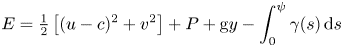 \begin{equation} E=\tfrac{1}{2}\left[(u-c)^{2}+v^{2}\right]+P+\mathrm{g} y-\int_0^{\psi}\gamma(s)\,\mathrm{d} s \end{equation}
which is a constant owing to conservation of energy. In the expression, g is gravitational acceleration,  $P$ is the pressure (normalized with respect to density) in the fluid and at the surface $P=P_{atm}$, the atmospheric pressure which also normalized with respect to density. Therefore, for a given water depth, we can introduce another constant $Q=2(E-P_{atm}+\mathrm {g} d)$, and the boundary condition on the surface is given by
 \begin{equation} \psi_x^{2}+\psi_y^{2}+2\mathrm{g}(y+d)=Q\quad\mbox{on}\ \psi=0. \end{equation}
Eventually, we obtain the fixed domain boundary-value problem from the free-surface wave problem by applying the following DJ transformation, i.e.
 \begin{equation} q=x\quad\mbox{and}\quad p=-\psi(x,y) \end{equation}
to the relations (2.5) and (2.7), and including the boundary condition at  $p=p_0$. The equations are
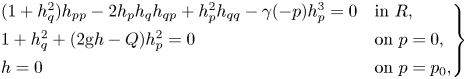 \begin{align} \left.\begin{array}{ll@{}} (1+h_q^{2})h_{pp}-2h_ph_qh_{qp}+h_{p}^{2}h_{qq}-\gamma(-p)h_p^{3}=0 & \mbox{in}\ R,\\ 1+h_q^{2}+(2\mathrm{g} h-Q)h_p^{2}=0 & \mbox{on}\ p=0,\\ h=0 & \mbox{on}\ p=p_0, \end{array}\right\} \end{align}
where  $h(q,p)=y+d$ is the height function and $R$ is the rectangle defined by $R=\{(q,p):-L < q < L,p_0 < p < 0\}$.
2.2. Recovery of wave properties
We will solve the problem (2.9) for the height function using a numerical method that will be introduced in the next section. For characterizing the waves, we shall recall the recovery of wave properties from the height function. Since in this formulation, the mean water depth  $d$ is not fixed, it needs to be recovered first from $h$ by
 \begin{equation} d=\frac{1}{2L}\int_{-L}^{L}h(q,0)\,\mathrm{d} q. \end{equation}
Afterwards, the water profile is determined by
 \begin{equation} y=h-d. \end{equation}
The wave height  $a$ is obtained as
 \begin{equation} a=h(0,0)-h(L,0) \end{equation}
as we are concerned with waves of one crest and one trough per period. Further, the velocity field is recovered by
 \begin{equation} (c-u,v)=\left(\frac{1}{h_p},-\frac{h_q}{h_p}\right), \end{equation}
recalling the DJ transformation (see Constantin (Reference Constantin2011) for details). The pressure in the fluid domain can be obtained from the relation (2.6) and here we define a relative pressure,  $\tilde P=P-P_{atm}$, for the following discussions as
 \begin{align} \tilde P &= -\frac{1+h_q^{2}}{2h^{2}_p}-\mathrm{g} h+\frac{Q}{2}-\int_{0}^{p} \gamma(-s)\,\mathrm{d} s = -\frac{\left[(u-c)^{2}+v^{2}\right]}{2}-\mathrm{g} (y+d) \nonumber\\ &\quad +\frac{Q}{2}-\int_0^{p}\gamma(-s)\,\mathrm{d} s. \end{align}
For computing water particle paths or trajectories, the travelling speed of the wave is recovered (Constantin Reference Constantin2011) by using
 \begin{equation} c= \kappa-\frac{1}{L}\int_0^{L} \left[u(x,-d)-c\right]\mathrm{d} \kern0.7pt x, \end{equation}
where  $\kappa$ is the average horizontal current strength on the bed. We then need to solve a set of differential equations (Constantin & Strauss Reference Constantin and Strauss2010; Nachbin & Ribeiro-Junior Reference Nachbin and Ribeiro-Junior2014)
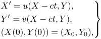 \begin{equation} \left.\begin{aligned} & X^{\prime}=u(X-ct,Y),\\ & Y^{\prime}=v(X-ct,Y),\\ & (X(0),Y(0))=(X_0,Y_0), \end{aligned}\right\} \end{equation}
where the prime denotes the derivative with respect to time. Here, we use a numerical integration method to compute the particle paths once the velocity field is solved, as will be detailed in the next section.
3. Numerical methods
In this section, we briefly introduce the numerical methods to solve (2.9), for performing numerical continuation to arrive at the solution of waves in flows with closely approaching stagnation points, and for computing the particle trajectories from the velocity field in the Eulerian setting. The dispersion relations and the linearized solutions for local bifurcation from the laminar flow solutions to small-amplitude wave solutions are also recalled for the sake of completeness.
3.1. Discretization and implementation
Following the methods in Ko & Strauss (Reference Ko and Strauss2008b) and Amann & Kalimeris (Reference Amann and Kalimeris2018), we use a finite difference scheme to discretize the computational domain. Taking advantage of the symmetry of  $h$ function with respect to $q=0$ (Constantin, Ehrnström & Wahlén Reference Constantin, Ehrnström and Wahlén2007), we set the computational domain as a fixed rectangle $[0,L]\times [p_0,0]$ to improve the computation efficiency. We first discretize the domain using uniformly distributed grid points and then refine the grid size near the surface and the bottom under the crest ( $q=0$). In the case of discontinuous vorticity, we additionally refine the grid size near the location where the vorticity changes abruptly. We apply the central difference scheme at interior grid points, and at left and right boundary points by mirroring $h$ along $q=0$ and $q=L$, considering the periodicity and symmetry properties of the waves in absence of stagnation points. At the boundaries $p=0$ and $p=p_0$, we apply the backward and forward difference schemes, respectively. Note that the refinement is achieved by reducing the grid size smoothly so that the central difference still has a second-order accuracy, approximately.
For implementation, we use the open-source library Eigen (Guennebaud & Jacob Reference Guennebaud and Jacob2010) for solving the nonlinear algebraic equations subsequent to the finite difference discretization. We use the predictor–corrector method detailed in Amann & Kalimeris (Reference Amann and Kalimeris2018) for numerical continuation and write our own code on the basis of Eigen. In the following numerical analysis, we discretize the domain first by an equidistant  $250\times 750$ grid with additional refinement at locations where the stagnation point may occur. Following the refinement, the smallest grid size achieved is ${1/8}$th of the initial size prior to the mentioned refinement.
3.2. Dispersion relations and linearization solutions for local bifurcation
As previously mentioned, we focus on the discontinuous vorticity. The vorticity function is expressed as
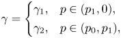 \begin{align} \gamma=\left\{\begin{array}{@{}ll} \gamma_1, & p\in(p_1,0),\\ \gamma_2, & p\in(p_0,p_1), \end{array}\right. \end{align}
where  $p_1$ corresponds to the value of the streamline at the interface $y=y_1$, and $\gamma _1$ and
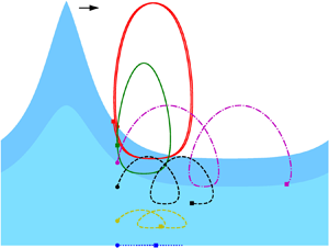
  $\gamma _2$ are the constant vorticity values of the surface layer and the layer adjacent to the bed. The setting of the problem is illustrated in figure 1. For the case of $\gamma _1=\gamma _2=0$, the problem reduces to irrotational flow, and the dispersion relation and the linearized solutions are available in Constantin (Reference Constantin2011). For the situation of a rotational flow over an irrotational and vice versa, the dispersion relations are explicitly derived in Constantin & Strauss (Reference Constantin and Strauss2011) and Constantin (Reference Constantin2012a), respectively. For steady water waves on two rotational layers, see Martin (Reference Martin2015).
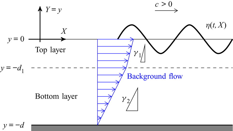
Figure 1. The setting of nonlinear periodic waves travelling on rotational flow with discontinuous vorticity. In the figure,  $\gamma _1$ and $\gamma _2$ are positive and $d_1$ denotes the thickness of the top layer.
The dispersion relations are nonlinear equations. Here, we solve them using the Newton method. For large vorticity, we apply a simple continuation scheme by using the solution for smaller vorticity for initialization (Seydel Reference Seydel2009).
3.3. Computation of the particle trajectories
We numerically compute the particle paths in the physical domain, i.e. in the fixed  $(X,Y)$-coordinate. For a particle located at $(X(t),Y(t))$ at time $t$, its velocity is interpolated from the velocities at the neighbouring four grid points (following appropriate translation) using a similar interpolation method as in Umeyama (Reference Umeyama2012). The interpolation scheme is illustrated in figure 2. Note that in our case, the cell is of trapezoidal shape in the physical domain. Subsequently, we use numerical integration to solve the first-order differential equations (2.16). This simple interpolation scheme is found to be sufficiently accurate.
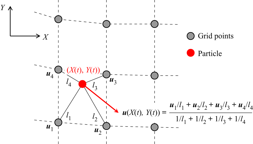
Figure 2. Interpolation strategy for instantaneous particle velocity. In the figure,  $\boldsymbol {u}=[u\enspace v]^{\top }$ is the velocity vector; $l_1, l_2, l_3$ and $l_4$ are respective distances of the particle to the four neighbouring grid points.
4. Results
Following Ko & Strauss (Reference Ko and Strauss2008a,Reference Ko and Straussb) and Amann & Kalimeris (Reference Amann and Kalimeris2018), we assign  $\mathrm {g}=9.8$, $2L=2{\rm \pi}$ and $p_0=-2$. We focus on the new part of the bifurcation curves, pressure distribution and particle paths under flows with nearly approaching stagnation points. Note that in the present system all the variables are expressed in SI units and a physical system of a different wavelength can be scaled to the $2{\rm \pi}$-periodic system analysed in this paper by scaling $\mathrm {g}$ and $\gamma$ using the wave number (Constantin Reference Constantin2011). However, the scaling has no influence on the laminar flow solution. In the following, as will be seen, the current velocity at the crest (under zero-amplitude waves) in most of the cases is less than 2.5 m s $^{-1}$, which is physically realistic in oceans.
4.1. Critical vorticity and the new part of the branch of bifurcation diagram
For the case of constant vorticity, it is known that when the vorticity is below a critical value  $\gamma _{crit}$, the stagnation point first appears at the bottom and at that stage numerical continuation breaks down (Ko & Strauss Reference Ko and Strauss2008b). However, Amann & Kalimeris (Reference Amann and Kalimeris2018) and Kalimeris (Reference Kalimeris2018) found that when $\gamma <\gamma _{crit}$ but is very close to $\gamma _{crit}$, the branch of the bifurcation diagram ( $a-Q$ plot) has another part which is bounded below and above by two values of the bifurcation parameter $Q$. These bounds correspond to two different waves in flows with stagnation point at the bottom and at the surface. On the new part of the branch, the wave height is further increased, and it is thus referred to as the upper part. To reach this upper part of the solutions, we need to overcome the gap of the bifurcation curve corresponding to waves in flows with stagnation points. For this purpose, Amann & Kalimeris (Reference Amann and Kalimeris2018) resorted to the $\gamma -$continuation scheme where a solution on the bifurcation diagram corresponding to $\gamma _0$ ( $\gamma _0>\gamma _{crit}>\gamma$) is used to initialize local bifurcation to arrive at one solution on the upper part corresponding to $\gamma$. Once one solution is obtained, the continuation in the solution set corresponding to $\gamma$ can be performed again with $Q$ or the wave height as the bifurcation parameter. In the following, we apply this scheme when needed.
Proceeding from the observations of Amann & Kalimeris (Reference Amann and Kalimeris2018), we investigated the case of discontinuous vorticity and found that the upper part also exists. Furthermore, for the case of discontinuous vorticity, the upper bound on this part always corresponds to waves in flows with the stagnation point at the surface, while its lower bound corresponds to waves in flows with stagnation point either at the bottom or at an internal point where vorticity jump occurs. We first show an example of the former situation. An irrotational flow ( $\gamma _1=0, p_1=-0.5$) was considered on a rotational flow with vorticity $\gamma _2$. We varied $\gamma _2$ to find out the critical value $\gamma _{2,crit}$ below which the stagnation point first occurs at the bottom. It was found that $\gamma _{2,crit}$ is slightly less than $-3.22$. Note that with the vorticity values $\gamma _1=0$ and $\gamma _2=-3.23$ and hence a shearing laminar flow with profile shown in figure 4(a) over a total water depth of 0.787 m, we have the surface velocity, $u=-2.07$ m s $^{-1}$ (the current flow direction is opposite to the wave propagation direction). Equation (2.5) with a bifurcation value of $Q = 26.85$ (see figure 3a) leads to the relative surface velocity with respect to the wave speed as $c-u=3.38$ m s $^{-1}$, since $u < c$. The wave speed $c$ is $1.31$ m s $^{-1}$ as also verified by the dispersion relation for this case. In the case of positive vorticity in the bottom layer, e.g. $\gamma _1=0$ and $\gamma _2=3$, the water depth is 0.74 m, the current velocity at the surface is approximately 1.53 m s $^{-1}$ and at the local bifurcation the wave speed is $c=3.69$ m s $^{-1}$. These values of the physical parameters indicate that the settings considered in this paper are realistic.
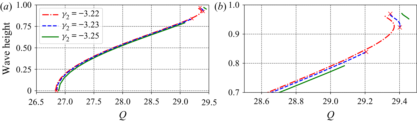
Figure 3. Bifurcation diagrams for cases with  $p_1=-0.5, \gamma _1=0$ (at the top layer) and various different values of $\gamma _2$ (at the bottom layer): (a) full diagrams; and (b) a close-up view of the upper parts.
We then further decreased  $\gamma _2$ and found the upper part, as shown in figure 3. For the case of $\gamma _2=-3.23$, the streamlines of wave solutions at the four endpoints (marked with crosses in figure 3) of the two parts of the bifurcation curve are shown in figure 4. Figure 4 clearly shows that the stagnation point first occurs at the bottom and then at the crest. Figure 5 shows the horizontal velocities $c-u$ at the bottom and at the surface under the crest along the bifurcation curves. Note that both waves in figures 4(b) and 4(c) correspond to flows close to having a stagnation point at the bottom, and the horizontal velocities $c-u$ at the bottom in these two cases are comparable, as in figure 5(a), while the wave in figure 4(c) has a larger height, a sharper crest and smaller horizontal velocity $c-u$ at the surface (see figure 5b). It is seen from figure 5 that the velocity $c-u$ at the bottom is first decreasing and then increasing along the bifurcation curve, with the presence of a gap for $\gamma _2<\gamma _{2,crit}$, while the velocity $c-u$ at the crest is decreasing monotonically. Indeed, at the uppermost end of the bifurcation diagram in all those three cases, the velocities $c-u$ at the surface are still larger than those at the bottom, the stagnation point is expected to occur at the crest because the velocity at the surface is decreasing while at the bottom is increasing with respect to the increasing wave height.
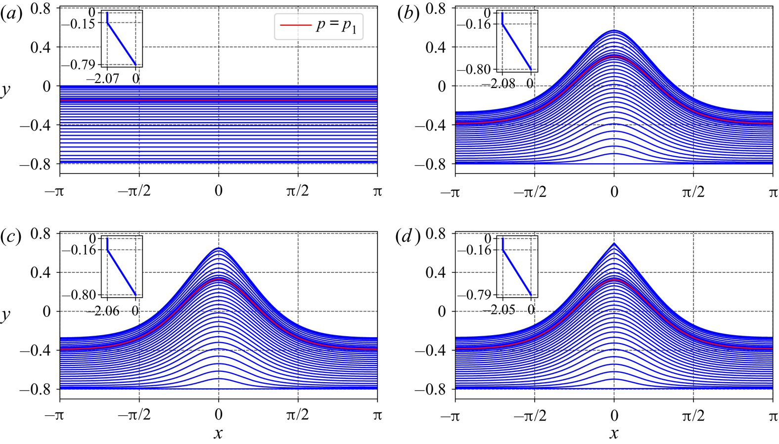
Figure 4. Streamlines of flows at the endpoints of each of the two parts of the bifurcation curve corresponding to  $p_1=-0.5, \gamma _1=0$ (at the top layer), and $\gamma _2=-3.23$ (at the bottom layer): (a) laminar flow; (b) wave at the upper bound of the lower part; (c) wave at the lower bound of the upper part; and (d) wave at the upper bound of the upper part. In the figures, the insets show the background current profile when there is no wave motion.

Figure 5. Horizontal velocity,  $c-u$, under the crest along the bifurcation curve for $\gamma _1=0$ (at the top layer), $p_1=-0.5$, and various different values of $\gamma _2$ (at the bottom layer): (a) at the bottom and (b) at the surface. In the figures, the insets are close-up views of the curves when approaching the largest wave height.
We further consider a layer ( $p_1=-0.7$) of rotational flow with vorticity $\gamma _1$ on an irrotational flow ( $\gamma _2=0$), following the setting in Ko & Strauss (Reference Ko and Strauss2008a) and Constantin & Strauss (Reference Constantin and Strauss2011). We found that the critical vorticity $\gamma _{1,crit}$ is slightly below $-10.41$ (a value refined from $-10$ in Ko & Strauss Reference Ko and Strauss2008a). By using $\gamma _1$ as the bifurcation parameter, we also found the upper part of the branch of the bifurcation diagram when $\gamma _1$ is less but very close to $\gamma _{1,crit}$. Figure 6 shows the bifurcation diagrams for $\gamma _1=-10.41, -10.42$ and $-10.45$. For $\gamma _1=-10.42$, the streamlines of the waves corresponding to the four endpoints of the bifurcation curve are shown in figure 7, which clearly illustrates that the stagnation point first occurs internally and later occurs at the crest with further increased wave height. Figure 8 shows the variation of the velocities $c-u$ at $p=p_1$ and at the surface along the bifurcation curves. The velocity $c-u$ at the position where vorticity jumps, is first decreasing and then increasing with respect to the wave height. Notably, the velocity decreases slightly again when close to the wave in flows with stagnation point at the surface. Again, the velocity $c-u$ on the crest is decreasing monotonically along with the increasing wave height.
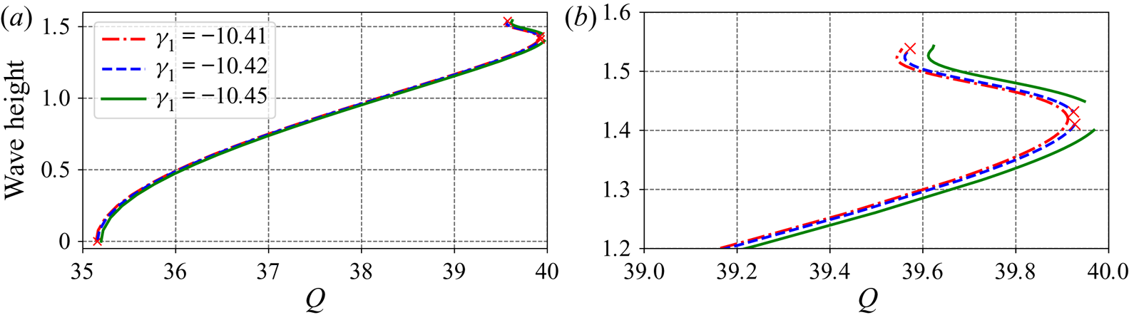
Figure 6. Bifurcation diagrams for cases with  $p_1=-0.7, \gamma _2=0$ (at the bottom layer) and various different values of $\gamma _1$ (at the top layer): (a) full diagrams; and (b) a close-up view of the upper parts.
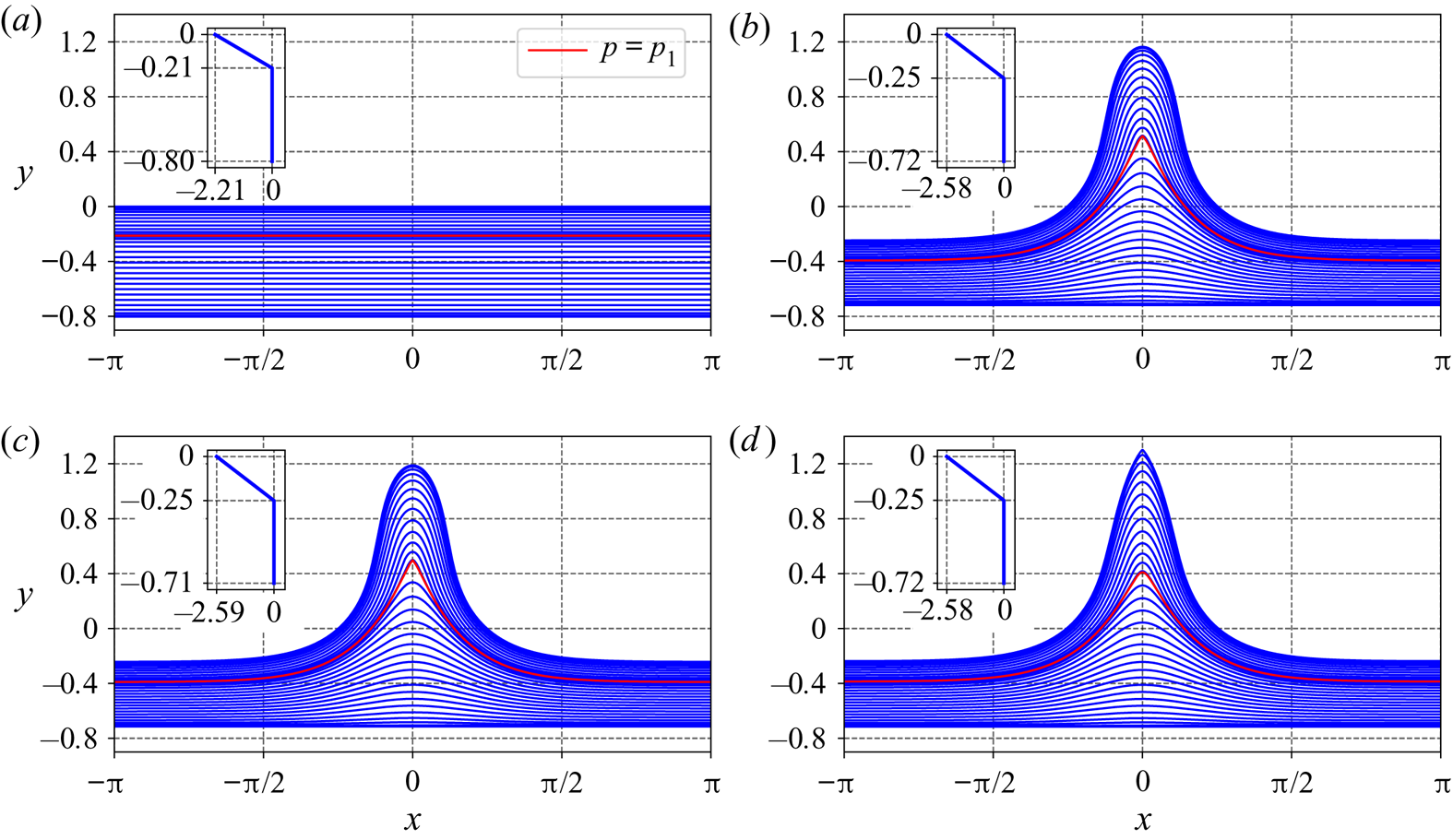
Figure 7. Streamlines of flows at the endpoints of each of the two parts of the bifurcation curve corresponding to  $p_1=-0.7$, $\gamma _1=-10.42$ (at the top layer), and $\gamma _2=0$ (at the bottom layer): (a) laminar flow; (b) wave at the upper bound of the lower part; (c) wave at the lower bound of the upper part; and (d) wave at the upper bound of the upper part. In the figures, the insets show the background current profile when there is no wave motion.

Figure 8. Horizontal velocity,  $c-u$, under the crest along the bifurcation curve for $\gamma _2=0$ (at the bottom layer), $p_1=-0.7$, and varying $\gamma _1$ (at the top layer): (a) at the position where vorticity jumps ( $y=y_1$ corresponds to $p=p_1$) and (b) at the surface. In the figures, the insets are close-up views of the curves when approaching the largest wave height.
To summarize, in this subsection, we have observed new features of the bifurcation curves with fixed mass flux, for large-amplitude waves on flows with discontinuous vorticity. Specifically, we show that along the bifurcation curve the stagnation point can first occur at the bottom or internally and then occur again at the surface for some particular vorticity distributions.
4.2. Pressure distribution
We now present the pressure distribution for waves with stagnation points at the bottom, at an internal position and at the surface, for the case with discontinuous vorticity.
For an irrotational flow on a rotational flow with  $p_1=-0.5$ and $\gamma _1=0$, we consider the cases corresponding to $\gamma _2=3, -2, -3.23$ and $-5$. For waves close to the case of flows having a stagnation point at the crest, the pressure distributions are shown in figure 9, and figure 10 compares the pressure along the bottom and along the crest line. For waves in flows close to having a stagnation point at the bottom, the pressure distribution demonstrated in figure 11, and figure 12 shows the pressure along the bottom and the crest line. Two features of the pressure distributions are consistent with the pressure beneath a Stokes wave as proved by Constantin & Strauss (Reference Constantin and Strauss2010) and those can be stated as ‘the pressure in the fluid strictly decreases horizontally away from a crest line toward its neighbouring trough lines, and the pressure strictly increases with depth’. Even though, when $\gamma _2$ is close to the critical value, the pressure along the bottom displays a ‘plateau’ behaviour, as previously pointed out by Amann & Kalimeris (Reference Amann and Kalimeris2018) for the case of constant vorticity, the pressure is still decreasing away from the crest line, slowly.
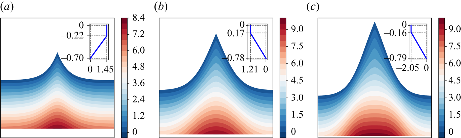
Figure 9. Pressure distribution for waves approaching waves with stagnation point at the crest for  $p_1=-0.5$, $\gamma _1=0$ (at the top layer), and: (a) $\gamma _2=3$; (b) $\gamma _2=-2$; and (c) $\gamma _2=-3.23$. In the figure, the insets show the corresponding background shear flow when there is no wave motion.
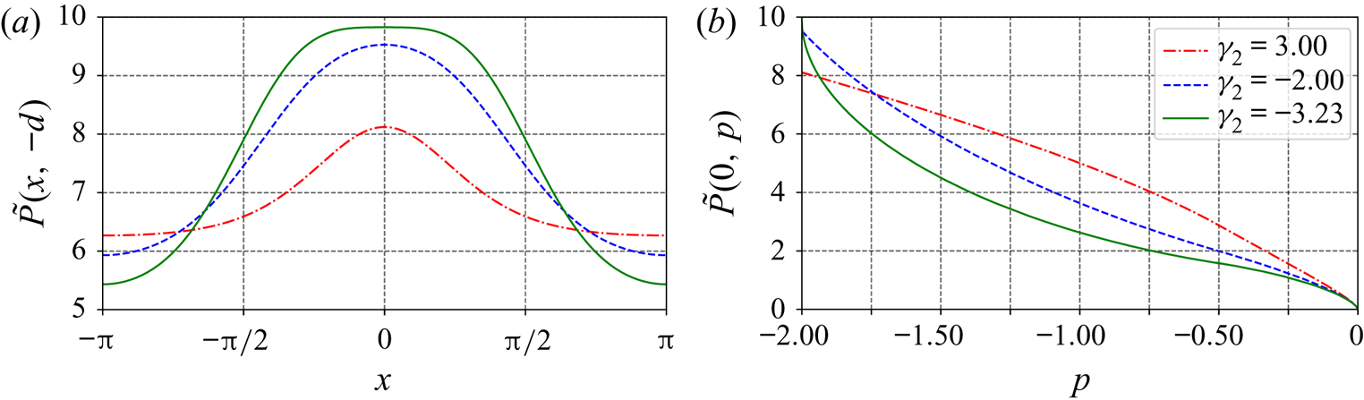
Figure 10. Pressure distribution in flows with an approaching stagnation point at the crest for  $p_1=-0.5$, $\gamma _1=0$ (at the top layer) and various different values of $\gamma _2$ along (a) the bottom, and (b) the crest line.
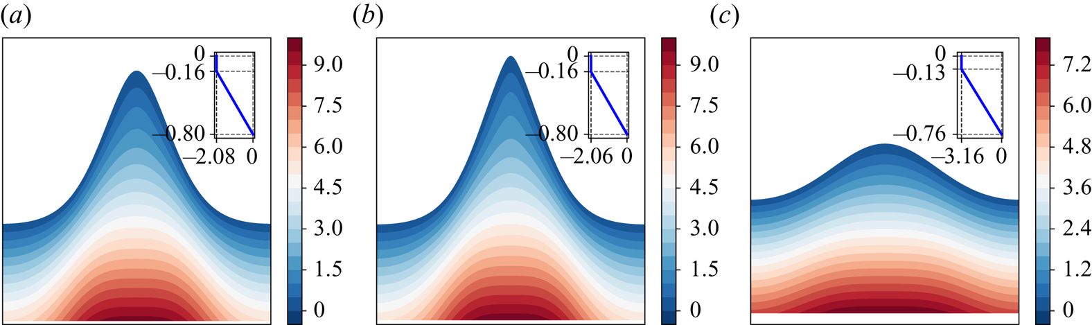
Figure 11. Pressure distribution in flows with an approaching stagnation point at the bottom for  $p_1=-0.5$, $\gamma _1=0$ (at the top layer), and: (a) $\gamma _2=-3.23$ (below gap); (b) $\gamma _2=-3.23$ (above gap); and (c) $\gamma _2=-5$. In the figure, the insets show the corresponding background shear flow when there is no wave motion.

Figure 12. Pressure distribution in flows with an approaching stagnation point at the bottom for  $p_1=-0.5$, $\gamma _1=0$ (at the top layer) and various different values of $\gamma _2$ along (a) the bottom, and (b) the crest line.
For a rotational flow on an irrotational flow, we analyse the cases for  $\gamma _1=5, -5, -10.42$ and $-12$. Figure 13 shows the pressure distribution in flows close to having a stagnation point at the crest, and variations of the pressure along the bottom and along the crest line are illustrated in figure 14. The pressure distribution in flows when internal stagnation points are almost developed is illustrated in figure 15. Correspondingly, figure 16 shows the pressure along the streamline $\psi =-p_1$ and along the crest line. From these figures, it is seen that none of the facts regarding the pressure distribution for an irrotational Stokes wave (Constantin & Strauss Reference Constantin and Strauss2010) hold, as also observed by Ribeiro, Milewski & Nachbin (Reference Ribeiro, Milewski and Nachbin2017) for rotational flows with constant vorticity. When the vorticity $\gamma _1$ is below a critical value, the pressure along the streamline $\psi =-p_1$ achieves a local minimum under the crest, as opposed to the maximum there when $\gamma _1$ is large. For smaller $\gamma _1$, the relative pressure $\tilde P$ at this position becomes negative (i.e. sub-atmospheric), which is the minimum along the streamline. The pressure attaining a value less than the atmospheric pressure has also been observed by Ali & Kalisch (Reference Ali and Kalisch2013) for the case of constant vorticity using a model based on an asymptotic expansion for the stream functions. When $\gamma _1$ is below a critical value, the pressure below but close to the layer where the vorticity jump occurs also exhibits the ‘plateau’ behaviour, internally, see figure 15. Figures 14–16 show that when $\gamma _1$ is much larger than the critical value, the pressure is increasing with depth along the crest line. Interestingly, when $\gamma _1$ is quite close to $\gamma _{1,crit}$, the pressure $\tilde P$ along the crest line first increases slightly, and then decreases, and increases again when close to the position where the vorticity jump occurs; the overall pressure in the surface layer is close to the atmospheric pressure, see figure 14(b) for $\gamma _1=-10.42$. With a further decrease in the value of $\gamma _1$ below the critical value, the relative pressure in the surface layer becomes negative, first decreasing from the crest and then increasing near the position where the vorticity jump takes place. To understand the reason for the development of a negative relative pressure $\tilde P$ in the surface layer near the crest line, we recall the expression (2.14). For the cases illustrated in figure 14, the term $\int _0^{p}\gamma (-s)\,\mathrm {d} s$ in (2.14) is positive in the surface layer and increases rapidly with depth since $|\gamma _1|$ is large, the term $\mathrm {g}(y+d)$ is also large considering the large wave height, and the velocity $c-u$ is also not small, as shown in figure 17; hence, $\tilde P$ in the surface layer becomes negative. Further decreasing $\gamma _1$ (with increasing $|\gamma _1|$), it seems that the minimal pressure along the crest line will keep decreasing.
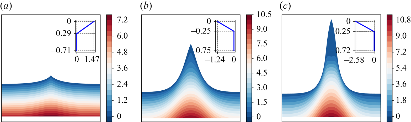
Figure 13. Pressure distribution in flows with an approaching stagnation point at the crest for  $p_1=-0.7$, $\gamma _2=0$ (at the bottom layer), and: (a) $\gamma _1=5$; (b) $\gamma _1=-5$; and (c) $\gamma _1=-10.42$. In the figure, the insets show the corresponding background shear flow when there is no wave motion.
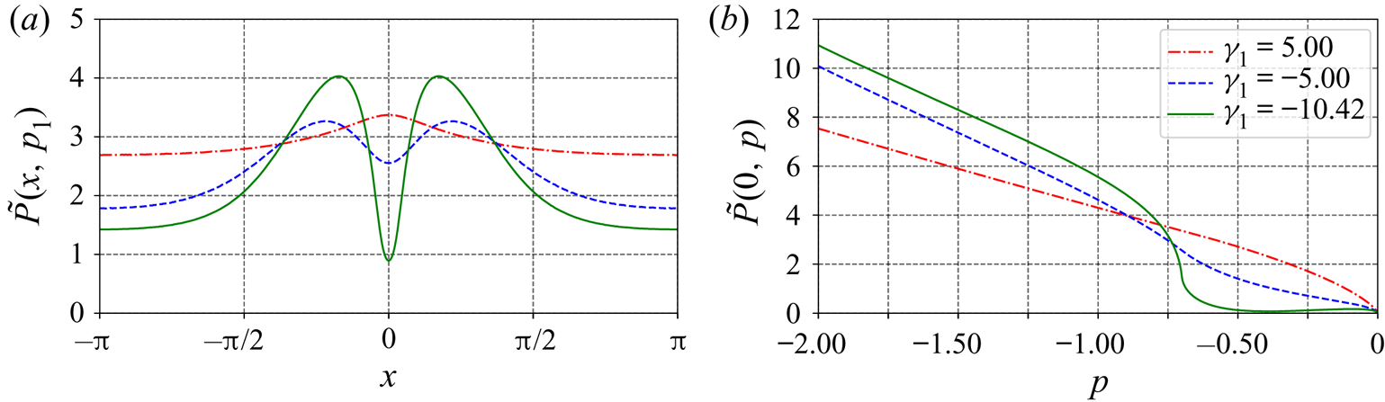
Figure 14. Pressure distribution in flows with an approaching stagnation point at the crest for  $p_1=-0.7$, $\gamma _2=0$ (at the bottom layer) and various different values of $\gamma _1$ along (a) the streamline $\psi =-p_1$, and (b) the crest line.

Figure 15. Pressure distribution in flows with an approaching stagnation point at a position where vorticity jump occurs, for  $p_1=-0.7$, $\gamma _2=0$ (at the bottom layer), and: (a) $\gamma _1=-10.42$ (below gap); (b) $\gamma _1=-10.42$ (above gap); and (c) $\gamma _1=-12$. In the figures, the insets show the background current profile when there is no wave motion.
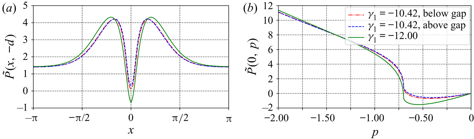
Figure 16. Pressure distribution in flows with an approaching stagnation point at a position where vorticity jump occurs for  $p_1=-0.7$, $\gamma _2=0$ and various different values of $\gamma _1$ along (a) the streamline $\psi =-p_1$, and (b) the crest line.
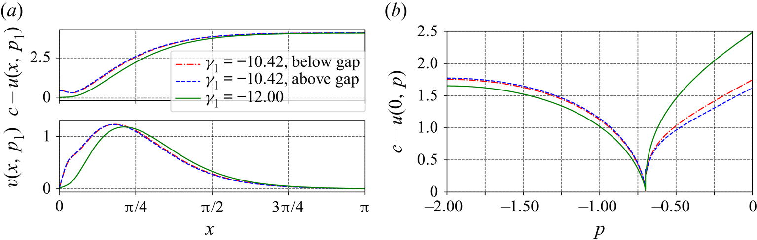
Figure 17. Variation of velocities,  $c-u$ and $v$, with $p_1=-0.7$, $\gamma _2=0$ (at the bottom layer), and various different values of $\gamma _1$: (a) $c-u$ and $v$ along the streamline $\psi =-p_1$, and (b) $c-u$ along the crest line ( $v$ is zero along this line and hence not shown).
4.3. Particle trajectories
We proceed by computing the particle trajectories under the waves corresponding to flows with nearly developed stagnation points, for the previously mentioned cases. To recover the wave speed using expression (2.15), we assume that the current strength at the bed is zero, i.e.  $\kappa =0$. Note that the choice of a different setting (adding an arbitrary uniform current) may lead to variations of the resulting particle paths. For example, when studying particle paths under waves on linear-shear flow, Ribeiro et al. (Reference Ribeiro, Milewski and Nachbin2017) set the current strength at the mid-depth to be zero (to ensure a flow with no net mass flux in the case of zero-amplitude waves). However, we here focus on the relative horizontal displacements of the particles along the depth, which are not affected by the presence of a uniform background current.
In the following computation and illustration of the particle trajectories, we set that: (i) the initial positions of the particles are under a zero-crossing point of the wave profile (Paprota & Sulisz Reference Paprota and Sulisz2018); (ii) the particles trajectories are plotted for the waves travelling rightwards for two wave periods, i.e. for a time of  $4L/c=4{\rm \pi} /c$, and the final position of the particles under zero-amplitude waves are also indicated in the graphs for comparison. In the graphs, six particle trajectories are plotted. Three of those particles are located at the surface, at the interface and at a position very close to the bottom but not exactly at the bottom. The other three particles include one located in the top layer and two located in the bottom layer. The initial positions are denoted by dots and the final positions are indicated by square markers.
First of all, we plot the computed particle trajectories in the moving frame, as illustrated in figure 18, which theoretically are the corresponding streamlines. The streamlines passing through the initial particle locations are plotted for comparison, and a good agreement is seen, suggesting the accuracy of the method for computing particle trajectories.
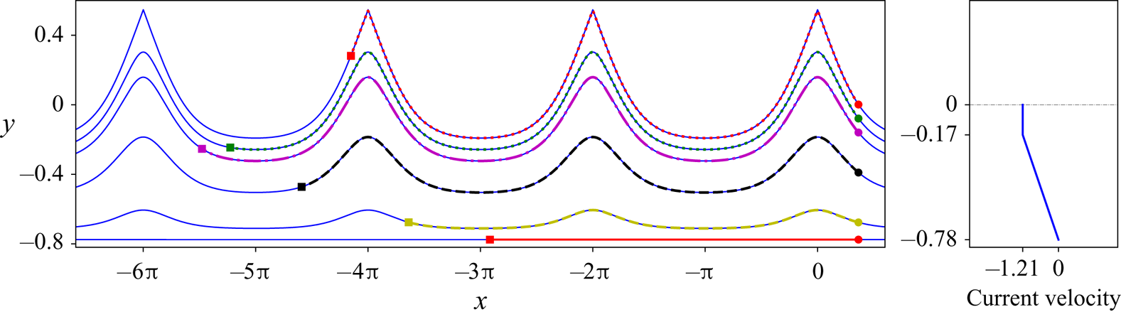
Figure 18. (a) Particle trajectories under the waves in flows close to having a stagnation point at the crest with  $p_1=-0.5$, $\gamma _1=0$, and $\gamma _2=-2$ in the moving frame; (b) the background current profile when there is no wave motion.
For an irrotational layer on a rotational layer, the particle trajectories in flows close to having a stagnation point at the crest are plotted in figure 19 and those in flows close to having a stagnation point at the bottom are plotted in figure 20. We show that as theoretically predicted by Constantin (Reference Constantin2006) when a particle reaches the crest of the wave in flows having a stagnation point at the crest, it does not pause there but moves further (figure 19a). However, for waves in flows close to having an internal stagnation point or a stagnation point at the bottom, a particle reaching the stagnation point tends to pause at that point in the moving frame, similar to the case shown in Ribeiro et al. (Reference Ribeiro, Milewski and Nachbin2017) for flows with a bottom stagnation point. Some observations on the features of the particle trajectories are listed below:
(i) In both figures 19 and 20, the horizontal positions of the particles are on the right of the grey lines (which are the positions of the particles with no waves), indicating that the waves induce a positive drift of the particles in the direction of the propagating waves. This is consistent with what was proved by Constantin (Reference Constantin2012b) and the experimental results (Paprota & Sulisz Reference Paprota and Sulisz2018) for irrotational flows.
(ii) In the top irrotational layer, the horizontal displacement (with respect to the background current induced displacement) or drift is larger when the particle is closer to the surface than when it is near the interface of the two layers, which is consistent with experimental and approximate theoretical results (Curtis et al. Reference Curtis, Carter and Kalisch2018; Paprota & Sulisz Reference Paprota and Sulisz2018). In the bottom rotational layer, when the vorticity is positive, the wave induced drift is larger when the particle is close to the interface as compared to the drift induced when the particle is close to the bottom surface. For negative (adverse) vorticity in the bottom layer, the largest drift tends to occur at the bottom surface (i.e. the bottom flat bed) when the flow is close to having a stagnation point at the bottom, as also observed in Ribeiro et al. (Reference Ribeiro, Milewski and Nachbin2017) for linear shear flow.
(iii) For flows close to having a stagnation point at the crest, as shown in figure 19, the negative vorticity in the bottom layer clearly increases the drift of the particles in the top irrotational layer relative to the background current, especially for particles at the surface.
(iv) For flows close to having a stagnation point at the bottom, as in figure 20, a stronger negative vorticity in the bottom layer tends to decrease the relative drifts of the particles at different vertical positions in the top layer, as observed by comparing figures 19(c) and 20(c).
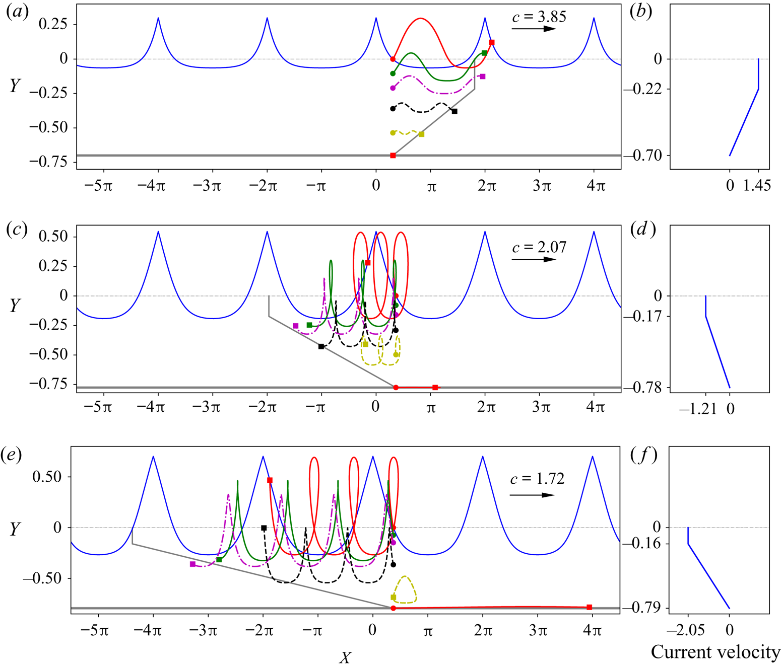
Figure 19. Particle trajectories under the waves in flows close to having a stagnation point near the crest, for  $p_1=-0.5$ and $\gamma _1=0$: (a) $\gamma _2=3$; (c) $\gamma _2=-2$; (e) $\gamma _2=-3.23$. The background current profiles corresponding to zero-amplitude waves are shown in (b,d,f), respectively. In the plot of the particle paths, the grey lines indicate the final position of the particles if under zero-amplitude waves after the time $4L/c$.
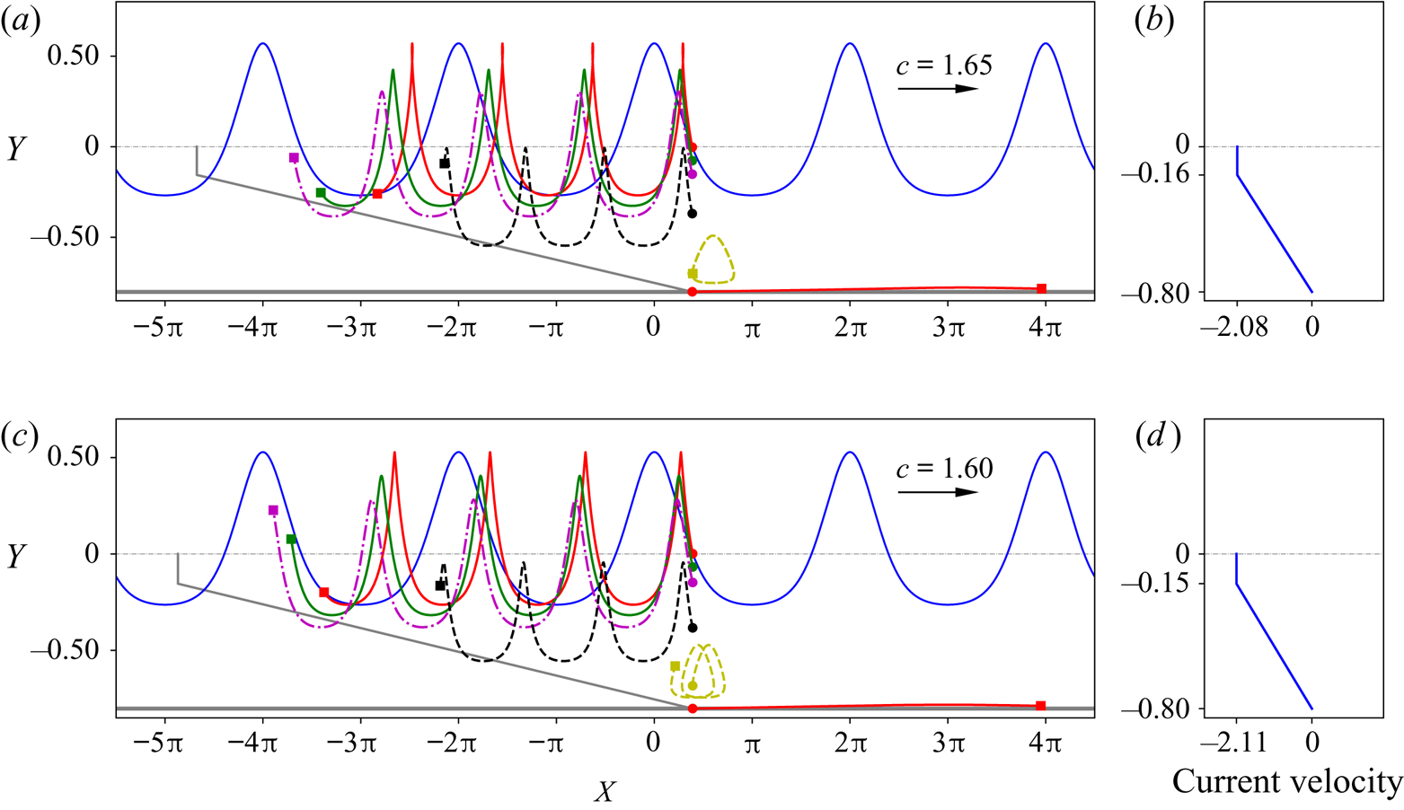
Figure 20. Particle trajectories under the waves in flows close to having a stagnation point at the bottom, for  $p_1=-0.5$ and $\gamma _1=0$: (a) $\gamma _2=-3.23$ (below the gap); (c) $\gamma _2=-3.25$ (below the gap). The background current profiles corresponding to zero-amplitude waves are shown in (b,d), respectively. In the plot of the particle paths, the grey lines indicate the final position of the particles if under zero-amplitude waves after the time $4L/c$.
With a shear layer on an irrotational layer, figure 21 shows the particle trajectories for flows close to having a stagnation point at the crest and figure 22 reveals the particle trajectories for flows close to having a stagnation point at the location when the vorticity jump occurs. Again, we can see from both figures that the wave-induced drifts are positive in the direction of the propagating waves. Some conspicuous features are observed as described below:
(i) In the bottom irrotational layer, the drift is always larger when the particle is close to the interface, consistent with particle paths in irrotational flow (Paprota & Sulisz Reference Paprota and Sulisz2018).
(ii) In the top rotational layer, when the vorticity is positive, the wave-induced drift is larger when the particle is near the surface as compared to the drift when the particle is close to the interface of the two layers; while with negative vorticity, for flows close to having a stagnation point at the interface, the particle with the largest drift is at the interface.
(iii) A negative vorticity in the top layer tends to increase the wave-induced drifts of particles in both layers.
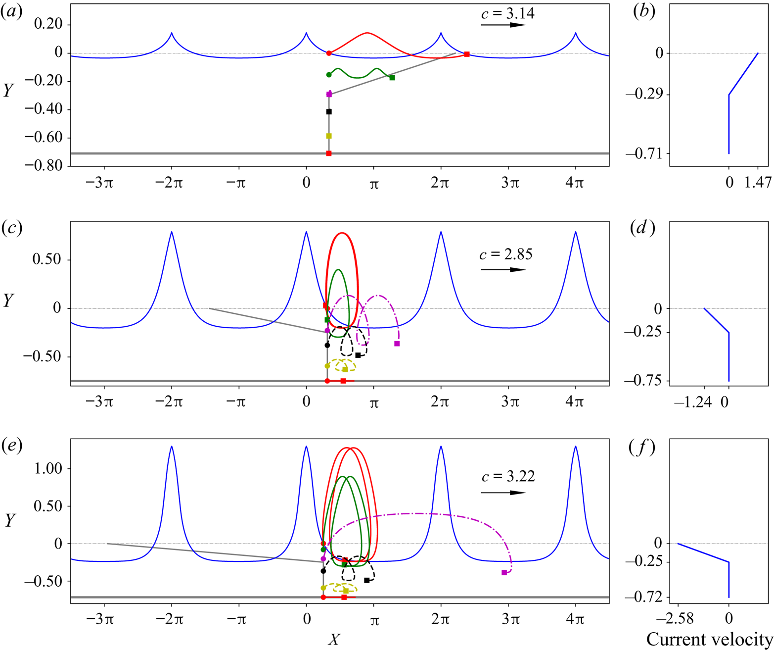
Figure 21. Particle trajectories under the waves in flows close to having a stagnation point near the crest, for  $p_1=-0.7$ and $\gamma _2=0$: (a) $\gamma _1=5$; (c) $\gamma _1=-5$; (e) $\gamma _1=-10.42$. The background current profiles corresponding to zero-amplitude waves are shown in (b,d,f), respectively. In the plot of the particle paths, the grey lines indicate the final position of the particles if under zero-amplitude waves after the time $4L/c$.
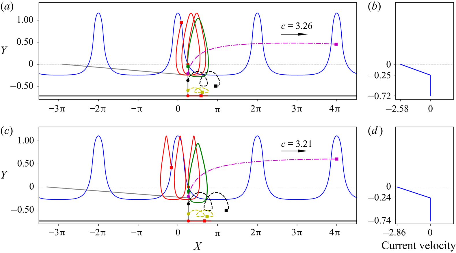
Figure 22. Particle trajectories under the waves in flows close to having a stagnation point at the bottom, for  $p_1=-0.7$ and $\gamma _2=0$: (a) $\gamma _2=-10.42$ (below the gap); (c) $\gamma _2=-12$. The background current profiles corresponding to zero-amplitude waves are shown in (b,d), respectively. In the plot of the particle paths, the grey lines indicate the final position of the particles if under zero-amplitude waves after the time $4L/c$.
5. Conclusions
In this paper, we investigate the behaviour of flow along a new bifurcation curve, and the pressure and particle trajectories under waves travelling on a rotational flow with discontinuous vorticity (close to having a stagnation point). For this purpose, we have developed a method for computing the particle paths using the velocity field obtained from a numerical continuation method based on DJ transform of the Euler equations for periodic waves on rotational flow. The continuation method generates a group of waves of fixed relative mass flux until a point where a flow with a stagnation point is reached.
By using the previously mentioned methods, we have recovered new branches of the bifurcation curves not connected to the trivial (laminar) solution, for waves on rotational flow with discontinuous vorticity. Particularly, we show that along the bifurcation curves, the stagnation point can first occur at the position where the vorticity jumps and then again occur at the surface. On the pressure distribution, we show that for the case of shear layer on an irrotational layer, the pressure in the top layer under the crest could be less than the atmosphere pressure and the pressure in the top layer near the interface displays a ‘plateau’ behaviour when the vorticity is large with a negative sign (i.e. adverse). This ‘plateau’ behaviour of the pressure has only been observed along the bottom for linear-shear flow. We further show the particle trajectories in flows close to having a stagnation point for various cases and qualitatively discuss the influence of vorticity of the rotational layer on the drifts of the particles in both layers.
Acknowledgements
The authors are grateful to the anonymous reviewers for their comments and suggestions which helped us improve the paper. L.C. acknowledges the partial support of the National Natural Science Foundation of China (grant number: 51978506). C.-I.M. acknowledges the support of the Austrian Science Fund (FWF) through research grant P 30878-N32.
Declaration of interests
The authors report no conflict of interest.


 Open access