


1 Introduction
Recent technological applications related with the needle-free injection of drugs (Mitragotri Reference Mitragotri2006) or printing (Brown et al. Reference Brown, Brasz, Ventikos and Arnold2012; Basaran, Gao & Bhat Reference Basaran, Gao and Bhat2013; Delrot et al. Reference Delrot, Modestino, Gallaire, Psaltis and Moser2016; Jalaal et al. Reference Jalaal, Schaarsberg, Visser and Lohse2019) resort to the impulsively generated and highly focused jets produced either after the sudden acceleration of a liquid column limited by a curved meniscus (Antkowiak et al. Reference Antkowiak, Bremond, Le Dizes and Villermaux2007; Kiyama et al. Reference Kiyama, Tagawa, Ando and Kameda2016) or by the velocities induced by the rapidly expanding vapour bubble created after the almost instantaneous vaporization of the liquid or solid volume absorbing a concentrated laser pulse (Tagawa et al. (Reference Tagawa, Oudalov, Visser, Peters, van der Meer, Sun, Prosperetti and Lohse2012), Peters et al. (Reference Peters, Tagawa, Oudalov, Sun, Prosperetti, Lohse and van der Meer2013), Brasz et al. (Reference Brasz, Arnold, Stone and Lister2015), Delrot et al. (Reference Delrot, Modestino, Gallaire, Psaltis and Moser2016), Kyriazis, Koukouvinis & Gavaises (Reference Kyriazis, Koukouvinis and Gavaises2019), Turkoz et al. (Reference Turkoz, Kang, Du, Deike and Arnold2019), Oyarte Galvez et al. (Reference Oyarte Galvez, Fraters, Offerhaus, Versluis, Hunter and Fernandez Rivas2020), see figure 1a left). This type of unsteady liquid ligament, which can even reach supersonic velocities (Tagawa et al. Reference Tagawa, Oudalov, Visser, Peters, van der Meer, Sun, Prosperetti and Lohse2012), experience a strong stretching in the downstream direction until a drop, with a noticeably smaller diameter than the width of the cavity from which the jet emanates, is ejected from its tip (see figure 1b). These unique features of highly focused transient jets make them suitable to spread high viscosity liquids over a substrate (Onuki, Oi & Tagawa (Reference Onuki, Oi and Tagawa2018), see figure 1a right) or to deliver, in a controlled manner, tiny amounts of drugs after the fast and thin jet penetrates the patient’s skin (Tagawa et al. Reference Tagawa, Oudalov, Ghalbzouri, Sun and Lohse2013).
Motivated by the number of emerging applications described above, here we provide a theoretical model describing the inception and subsequent dynamics of the impulsive jets emerging from the base of a curved interface. Our theoretical results reveal that, for given material properties of the liquid, the ejection and subsequent spatio-temporal evolution of the jet can be described in terms of just the local values around the axis of symmetry of the initial distribution of normal liquid velocities at the locally spherical surface. Indeed, if the distribution of normal velocities were uniform, the interface would be deformed preserving the spherical symmetry, not giving rise to the emergence of a jet, as will become clear in the following section.
The paper is structured as follows: in § 2 we present the theoretical results and compare the predictions with both our own experimental results and with those found in the literature and § 3 is devoted to summarize our main findings in this contribution.
2 Theory and comparison with experiments
The fast and thin vertical jets observed in many different natural flows, like those appearing when a solid impacts a liquid pool (Gekle & Gordillo Reference Gekle and Gordillo2010) or after a bubble floating on a free surface bursts (Duchemin et al. Reference Duchemin, Popinet, Josserand and Zaleski2002; Gordillo & Rodríguez-Rodríguez Reference Gordillo and Rodríguez-Rodríguez2019; Blanco-Rodríguez & Gordillo Reference Blanco-Rodríguez and Gordillo2020), have their origin in the mass conservation of the radial inflow generated by the implosion of the cavity walls, this being the reason why these types highly unsteady flows can be modelled theoretically as the ones induced by a distribution of sinks located at the axis of symmetry. Similarly, the type of high-speed jets emerging from the base of a curved interface like the one depicted in figure 1(b), arise as a result of the constancy of the liquid flow rate of mean velocity  $V$ created by either the sudden acceleration of a liquid column or by the expansion of the gas vapour bubble produced by the almost instantaneous evaporation of a certain volume of liquid (see figure 1a).

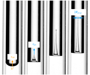
Figure 1. (a) Sketch of the two methods used here to generate the impulsive liquid jet: the left image illustrates the case in which the jet formation process is triggered by focusing a laser pulse on a liquid filled tube, whereas the right one corresponds to the case in which the jet is generated using the more complex geometry reported by Onuki et al. (Reference Onuki, Oi and Tagawa2018), when a metal rod is shot up by a coil gun upwards, impacting the tube. (b) Sequence showing the temporal evolution of the impulsively generated jet using the type of device described in Onuki et al. (Reference Onuki, Oi and Tagawa2018). The blue scale bar indicates 1 mm. (c) Illustration of the different variables used to describe the jet ejection process. (d) Sketch of the device proposed in Onuki et al. (Reference Onuki, Oi and Tagawa2018) to generate the impulsive liquid jet.
Given the local nature of the flow focusing effect to be described in what follows, from now on, and without loss of generality, we will refer to the physical situation depicted in figure 1(c), which sketches a spherical meniscus with a radius of curvature  $R_{c}=R_{t}/\cos \unicode[STIX]{x1D703}$ of a liquid of density $\unicode[STIX]{x1D70C}$, viscosity $\unicode[STIX]{x1D707}$ and interfacial tension coefficient $\unicode[STIX]{x1D70E}$ forming a contact angle $\unicode[STIX]{x1D703}$ with a cylindrical tube of radius $R_{t}$. The origin for time is set at the instant the mean liquid velocity with respect to the tube walls, $V$, is imposed upstream of the meniscus and, in the following, we will consider that the hydrodynamic time characterizing the jet formation process, $T_{h}$, is much smaller than the typical time of variation of $V$. Moreover, we will restrict our study to the case of liquids with viscosities such that the boundary layer thickness verifies the condition $\sqrt{(\unicode[STIX]{x1D707}/\unicode[STIX]{x1D70C})T_{h}}\ll R_{t}$, a fact implying that the liquid velocity profile upstream of the curved interface can be considered as uniform, as it is sketched in figure 1(c). Dimensionless variables, represented here using lower case letters to differentiate them from their dimensional counterparts (in capitals), are defined using $R_{t}$, $V$ and $\unicode[STIX]{x1D70C}V^{2}$ as the characteristic dimensions of length, velocity and pressure, respectively. The variables $z$ and $r$ depicted in figure 1(c) indicate the axial and radial coordinates, $\unicode[STIX]{x1D712}(\unicode[STIX]{x1D713},t)$ is the distance measured from the centre of the initial cavity to the free interface, $\unicode[STIX]{x1D713}$ is azimuthal angle in spherical coordinates and $h(\unicode[STIX]{x1D713},t)$ is the vertical distance measured from the base of the initially spherical cavity (see figure 1c). Notice that $\unicode[STIX]{x1D712}(\unicode[STIX]{x1D713},t=0)=1/\cos \unicode[STIX]{x1D703}=r_{c}$. Here we will only focus on the description of those experimental conditions in which the flow field in the neighbourhood of the free surface can be described using the incompressible approach and exclude the possibility that cavitation bubbles appear, as it was reported in Kiyama et al. (Reference Kiyama, Tagawa, Ando and Kameda2016).
Then, since viscous effects can be neglected under the conditions indicated above, the initial normal velocity distribution at the interface can be found by solving the Laplace equation  $\unicode[STIX]{x1D6FB}^{2}\unicode[STIX]{x1D719}=0$ for the velocity potential $\unicode[STIX]{x1D719}$, subjected to the impenetrability condition at the walls $\unicode[STIX]{x2202}\unicode[STIX]{x1D719}/\unicode[STIX]{x2202}n=0$ ( $n$ is the normal distance to the wall), to the condition $\unicode[STIX]{x2202}\unicode[STIX]{x1D719}/\unicode[STIX]{x2202}z=1$ at the boundary where the flow rate is imposed and to the Euler–Bernoulli equation at the free interface, which reduces to $\unicode[STIX]{x1D719}=0$. The straightforward numerical solution of the Laplace equation in the simple geometrical domain sketched in figure 1(c) or in other more complex geometries such as those reported in Onuki et al. (Reference Onuki, Oi and Tagawa2018) (see figure 1d) provides us with the initial normal velocity distribution at the interface $v_{r}(r=r_{c},\unicode[STIX]{x1D713},t=0)=-\unicode[STIX]{x2202}\unicode[STIX]{x1D719}/\unicode[STIX]{x2202}r(r=r_{c},\unicode[STIX]{x1D713},t=0)$ which, due to the fact that $\unicode[STIX]{x2202}v_{r}/\unicode[STIX]{x2202}\unicode[STIX]{x1D713}(\unicode[STIX]{x1D713}=0)=0$, can be expressed, in the neighbourhood of the axis of symmetry as
 $$\begin{eqnarray}v_{r}(r=r_{c},\unicode[STIX]{x1D713},t=0)=v_{n0}(\unicode[STIX]{x1D703})\cos (k(\unicode[STIX]{x1D703})\unicode[STIX]{x1D713})\quad \text{for}~\unicode[STIX]{x1D713}\ll 1,\end{eqnarray}$$
 where  $v_{n0}(\unicode[STIX]{x1D703})=v_{r}(r=r_{c},\unicode[STIX]{x1D713}=0,t=0)$ and $k(\unicode[STIX]{x1D703})$ are functions of the contact angle $\unicode[STIX]{x1D703}$. Notice that $k>0$, which quantifies the variation of the initial radial velocity along the azimuthal direction $\unicode[STIX]{x1D713}$, is calculated from the numerical solution of the Laplace equation, which provides us with the function $v_{r}(\unicode[STIX]{x1D713},t=0,r=r_{c})$. Indeed, the differentiation of (2.1) twice by $\unicode[STIX]{x1D713}$ yields
 $$\begin{eqnarray}k^{2}=-\frac{1}{v_{n0}}\frac{\unicode[STIX]{x2202}^{2}v_{r}}{\unicode[STIX]{x2202}\unicode[STIX]{x1D713}^{2}}(\unicode[STIX]{x1D713}=0,t=0,r=r_{c}).\end{eqnarray}$$
 The initial jet velocity with respect to the tube walls,  $v_{jet}$ is, however, larger than $v_{n0}$ in (2.1) due to the flow focusing effect described in Milgram (Reference Milgram1969), Antkowiak et al. (Reference Antkowiak, Bremond, Le Dizes and Villermaux2007), Tagawa et al. (Reference Tagawa, Oudalov, Visser, Peters, van der Meer, Sun, Prosperetti and Lohse2012) and Peters et al. (Reference Peters, Tagawa, Oudalov, Sun, Prosperetti, Lohse and van der Meer2013). In order to quantitatively predict the velocity at which the jet is initially ejected, we take into account that, since the flow field is initially perpendicular to the interface and, moreover, the liquid inertia in the tube guarantees the constancy of the flow rate during the jet ejection process, the integration of the continuity equation in spherical coordinates provides us with the following equation for the radial velocity field:
 $$\begin{eqnarray}v_{r}(r,\unicode[STIX]{x1D713},t)=\frac{v_{n0}\cos (k\unicode[STIX]{x1D713})r_{c}^{2}}{r^{2}}.\end{eqnarray}$$
Equation (2.3) and the kinematic condition at the interface
 $$\begin{eqnarray}\frac{\text{d}\unicode[STIX]{x1D712}(\unicode[STIX]{x1D713},t)}{\text{d}t}=-v_{r}(r=\unicode[STIX]{x1D712},\unicode[STIX]{x1D713},t)\end{eqnarray}$$
provide us with the following equation for the time-evolving position of the free interface:
 $$\begin{eqnarray}\frac{\unicode[STIX]{x1D712}(\unicode[STIX]{x1D713},t)}{r_{c}}=\left(1-3\frac{v_{n0}}{r_{c}}\cos (k\unicode[STIX]{x1D713})t\right)^{1/3}.\end{eqnarray}$$
 The accuracy of expressions in (2.3) and (2.5) could be improved by adding first-order correction terms, linear in  $t$, accounting for the fact that the value of potential $\unicode[STIX]{x1D719}$ at the moving free interface needs to be updated using the Euler–Bernoulli equation. However, the simplified description provided by (2.3)–(2.5) will prove to be sufficiently accurate to not only predict the initial jet velocity, but also the subsequent stretching of the jet and the diameter of the ejected droplet, as it will be shown in what follows.
Our analysis continuous by finding the expression of the time-varying vertical position of the free surface  $h$ (see figure 1c),
 $$\begin{eqnarray}\frac{h(\unicode[STIX]{x1D713},t)}{r_{c}}=1-\cos (\unicode[STIX]{x1D713})\frac{\unicode[STIX]{x1D712}(\unicode[STIX]{x1D713},t)}{r_{c}}=1-\cos (\unicode[STIX]{x1D713})\left(1-3\frac{v_{n0}}{r_{c}}\cos (k\unicode[STIX]{x1D713})t\right)^{1/3}.\end{eqnarray}$$
 As a next step, we notice that the instant at which the jet emerges is determined from the condition that there must exist a maximum elevation of the interface at the axis of symmetry. Since equation  $\unicode[STIX]{x2202}h/\unicode[STIX]{x2202}\unicode[STIX]{x1D713}(\unicode[STIX]{x1D713}\ll 1)=0$ reads
 $$\begin{eqnarray}\left(1-3\cos (k\unicode[STIX]{x1D713})\frac{v_{n0}}{r_{c}}t\right)-k\frac{\sin (k\unicode[STIX]{x1D713})}{\tan (\unicode[STIX]{x1D713})}\frac{v_{n0}}{r_{c}}t=0,\end{eqnarray}$$
 the instant  $t^{\ast }$ when the jet is ejected from the base of the curved cavity, where $\cos (k\unicode[STIX]{x1D713})=1$ and $\sin (k\unicode[STIX]{x1D713})/\tan (\unicode[STIX]{x1D713})=k$, is given by
 $$\begin{eqnarray}\unicode[STIX]{x1D70F}^{\ast }=\frac{1}{3+k^{2}}\quad \text{with}~\unicode[STIX]{x1D70F}^{\ast }=\frac{v_{n0}}{r_{c}}t^{\ast }.\end{eqnarray}$$
 The substitution of the value of  $\unicode[STIX]{x1D70F}^{\ast }$ in (2.8) into (2.3) and (2.5) particularized at $\unicode[STIX]{x1D713}=0$, yields
 $$\begin{eqnarray}v_{jet}=v_{r}(r=\unicode[STIX]{x1D712},\unicode[STIX]{x1D713}=0,t=t^{\ast })=v_{n0}\left(\frac{k^{2}}{3+k^{2}}\right)^{-2/3},\end{eqnarray}$$
 with the values of  $v_{n0}$ and $k^{2}$ calculated from the solution of the Laplace equation subjected to the boundary conditions detailed above.
To predict the spatio-temporal evolution of the tip of the jet for  $t>t^{\ast }$, we make use of the fact that, since the jet is slender and the characteristic Weber number verifies the condition $We=\unicode[STIX]{x1D70C}V^{2}v_{jet}^{2}R_{t}/\unicode[STIX]{x1D70E}\gg 1$, capillary effects are subdominant and the equations governing the flow can be approximated by those given in Gekle & Gordillo (Reference Gekle and Gordillo2010),
 $$\begin{eqnarray}\left.\begin{array}{@{}c@{}}\displaystyle \frac{\unicode[STIX]{x2202}r_{j}^{2}}{\unicode[STIX]{x2202}t}+\frac{\unicode[STIX]{x2202}}{\unicode[STIX]{x2202}z}(r_{j}^{2}u)=0\Rightarrow \frac{\text{D}}{\text{D}t}(\ln r_{j}^{2})=-s\quad \text{with}~s=\frac{\unicode[STIX]{x2202}u}{\unicode[STIX]{x2202}z}\\ \displaystyle \frac{\unicode[STIX]{x2202}u}{\unicode[STIX]{x2202}t}+u\frac{\unicode[STIX]{x2202}u}{\unicode[STIX]{x2202}z}=0\Rightarrow \frac{\text{D}u}{\text{D}t}=0,\end{array}\right\}\end{eqnarray}$$
 with  $r_{j}$ and $u$ indicating, respectively, the jet radius and the axial liquid velocity, $\text{D}/\text{D}t\equiv \unicode[STIX]{x2202}/\unicode[STIX]{x2202}t+u\unicode[STIX]{x2202}/\unicode[STIX]{x2202}z$ denoting the material derivative and where the small corrections associated with the capillary pressure gradient term have been neglected at this step of the derivation. In Blanco-Rodríguez & Gordillo (Reference Blanco-Rodríguez and Gordillo2020), the continuity equation in (2.10) is solved once the momentum equation in (2.10) is differentiated with respect to $z$ in order to obtain the following expression for the strain rate:
 $$\begin{eqnarray}\frac{\unicode[STIX]{x2202}}{\unicode[STIX]{x2202}z}\left(\frac{\unicode[STIX]{x2202}u}{\unicode[STIX]{x2202}t}+u\frac{\unicode[STIX]{x2202}u}{\unicode[STIX]{x2202}z}\right)=0\Rightarrow \frac{\text{D}s}{\text{D}t}+s^{2}=0\Rightarrow -\frac{\text{D}s}{s^{2}}=\text{D}t\Rightarrow s=\frac{s_{0}(\unicode[STIX]{x1D70F})}{1+(t-\unicode[STIX]{x1D70F})s_{0}(\unicode[STIX]{x1D70F})},\end{eqnarray}$$
 with  $t\geqslant t^{\ast }$, $\unicode[STIX]{x1D70F}\leqslant t$ a parameter and $s_{0}(\unicode[STIX]{x1D70F})$ the time-evolving dimensionless strain rate at the spatial position where the jet meets the base of the cavity. The particularization of (2.11) at $\unicode[STIX]{x1D70F}=t^{\ast }$ ( $t=t^{\ast }$) provides us with the time evolution of the strain rate at the tip of the jet for $t>t^{\ast }$. The value of the strain rate at the instant of jet ejection, $s_{0}(\unicode[STIX]{x1D70F}=t^{\ast })$, can be calculated making use of (2.3)–(2.5) and (2.8), from where it is deduced that
 $$\begin{eqnarray}\displaystyle s_{0}(\unicode[STIX]{x1D70F}=t^{\ast }) & = & \displaystyle -\frac{\unicode[STIX]{x2202}v_{r}}{\unicode[STIX]{x2202}r}(r=\unicode[STIX]{x1D712},\unicode[STIX]{x1D713}=0,t=t^{\ast })\nonumber\\ \displaystyle & = & \displaystyle 2\frac{v_{r}}{r}(r=\unicode[STIX]{x1D712},\unicode[STIX]{x1D713}=0,t=t^{\ast })=\frac{2v_{jet}}{\unicode[STIX]{x1D712}(\unicode[STIX]{x1D713}=0,t=t^{\ast })}\nonumber\\ \displaystyle & = & \displaystyle \frac{2v_{n0}}{r_{c}}\frac{3+k^{2}}{k^{2}}.\end{eqnarray}$$
 Therefore, the substitution of (2.11) and (2.12) particularized at  $\unicode[STIX]{x1D70F}=t^{\ast }$ into the continuity equation in (2.10), yields the following expression for the time evolution of the radius of the tip of the jet:
 $$\begin{eqnarray}\frac{\text{D}}{\text{D}t}(\ln r_{j}^{2})=-\frac{s_{0}(\unicode[STIX]{x1D70F}=t^{\ast })}{1+(t-t^{\ast })s_{0}(\unicode[STIX]{x1D70F}=t^{\ast })}\Rightarrow r_{jet}=\frac{r_{j0}}{\sqrt{1+(t-t^{\ast })s_{0}(\unicode[STIX]{x1D70F}=t^{\ast })}},\end{eqnarray}$$
 with  $r_{j0}$ the jet radius at the instant of jet ejection, determined here using the characteristic local values of the liquid velocity and of the strain rate at the apex of the spherical cavity at $t=t^{\ast }$, namely,
 $$\begin{eqnarray}r_{j0}=\unicode[STIX]{x1D6FD}\frac{v_{n0}}{s_{0}(\unicode[STIX]{x1D70F}=t^{\ast })},\end{eqnarray}$$
 with  $\unicode[STIX]{x1D6FD}$ a constant of order unity, to be calculated in what follows from just one single experiment. Equations (2.2), (2.9), (2.12), (2.13) and (2.14) will describe the spatio-temporal evolution of the jet tip radius, but only during a finite interval of time. Indeed, equation (2.13) expresses that the tip radius continuously decreases in time and tends to $r_{j0}/\sqrt{ts_{0}}$ for $t\gg 1$ as a consequence of the fact that the local strain rate at the jet tip is always positive (see (2.11)). Hence, if the result expressed by (2.13) were valid for arbitrarily large values of $t$, the jet tip radius would tend to zero. However, this unphysical result is prevented thanks to capillarity, which decreases down to zero the value of the strain rate at the top part of the jet. Indeed, following the ideas in Gordillo & Gekle (Reference Gordillo and Gekle2010), the tip of the jet is decelerated by the action of capillary stresses as it is dictated by the momentum balance
 $$\begin{eqnarray}\unicode[STIX]{x1D70C}R_{t}^{2}V^{2}\frac{\text{d}v_{jet}}{\text{d}t}r_{jet}^{3}\propto -\unicode[STIX]{x1D70E}R_{t}r_{jet},\end{eqnarray}$$
from which it is possible to estimate the variation in time of the jet tip velocity as
 $$\begin{eqnarray}\unicode[STIX]{x0394}v_{jet}\propto -\frac{\unicode[STIX]{x1D70E}}{\unicode[STIX]{x1D70C}V^{2}R_{t}}\frac{t-t^{\ast }}{r_{jet}^{2}}.\end{eqnarray}$$
 The instant  $t_{bulb}$ at which a drop will start being formed is the one for which the liquid begins accumulating at the top part of the jet, this happening when the local strain rate at the tip of the jet changes sign from positive to negative. This condition, which would never be fulfilled in the absence of interfacial tension stresses, reads (Gordillo & Gekle Reference Gordillo and Gekle2010),
 $$\begin{eqnarray}sr_{jet}+\unicode[STIX]{x0394}v_{jet}\approx 0\Rightarrow \frac{\unicode[STIX]{x1D70E}}{\unicode[STIX]{x1D70C}V^{2}R_{t}}\frac{t_{bulb}-t^{\ast }}{r_{jet}^{2}}\approx \frac{s_{0}(t^{\ast })}{1+(t_{bulb}-t^{\ast })s_{0}(t^{\ast })}r_{jet},\end{eqnarray}$$
 with  $s$ and $\unicode[STIX]{x0394}v_{jet}$ in (2.17) given, respectively, by (2.11) and (2.16). In the limit $(t_{bulb}-t^{\ast })s_{0}\gg 1$, the instant $t_{bulb}$ at which drop formation begins can be deduced from (2.17) as
 $$\begin{eqnarray}(t_{bulb}-t^{\ast })^{2}s_{0}^{2}[1+(t_{bulb}-t^{\ast })s_{0}]^{3/2}\propto \frac{\unicode[STIX]{x1D70C}V^{2}R_{t}}{\unicode[STIX]{x1D70E}}s_{0}^{2}r_{j0}^{3}\Rightarrow (t_{bulb}-t^{\ast })s_{0}\propto (We\,s_{0}^{2}r_{j0}^{3})^{2/7},\end{eqnarray}$$
with
 $$\begin{eqnarray}We=\frac{\unicode[STIX]{x1D70C}V^{2}R_{t}}{\unicode[STIX]{x1D70E}}\end{eqnarray}$$
 and where use of (2.13) for  $r_{jet}$ has been made. Inserting (2.18) into (2.13) provides us with $r_{bulb}$, namely, the radius of the jet at the instant $t_{bulb}-t^{\ast }$,
 $$\begin{eqnarray}r_{bulb}\propto r_{j0}(We\,s_{0}^{2}r_{j0}^{3})^{-1/7}.\end{eqnarray}$$
 Then, since the characteristic breakup time of the jet is the capillary time, the dimensionless instant  $t_{drop}$ at which a drop will be issued from the tip of the jet is given by
 $$\begin{eqnarray}\displaystyle (t_{drop}-t^{\ast })s_{0} & {\approx} & \displaystyle (t_{bulb}-t^{\ast })s_{0}+\frac{V}{R_{t}}\left(\frac{\unicode[STIX]{x1D70C}R_{t}^{3}r_{bulb}^{3}}{\unicode[STIX]{x1D70E}}\right)^{1/2}s_{0}\approx (We\,s_{0}^{2}r_{j0}^{3})^{2/7}+We^{1/2}r_{bulb}^{3/2}s_{0}\nonumber\\ \displaystyle & \Rightarrow & \displaystyle (t_{drop}-t^{\ast })s_{0}\propto (We\,s_{0}^{2}r_{j0}^{3})^{2/7},\end{eqnarray}$$
where use of (2.20) has been made. Therefore, the radius of the drop can be calculated inserting (2.21) into (2.13),
 $$\begin{eqnarray}r_{drop}\propto r_{j0}(We\,s_{0}^{2}r_{j0}^{3})^{-1/7},\end{eqnarray}$$
a result that recovers the one deduced in Gordillo & Gekle (Reference Gordillo and Gekle2010),
 $$\begin{eqnarray}R_{drop}\simeq KR_{t}r_{j0}\,We_{S}^{-1/7}\quad \text{with}~We_{S}=\frac{\unicode[STIX]{x1D70C}V^{2}R_{t}}{\unicode[STIX]{x1D70E}}s_{0}^{2}r_{j0}^{3}=We\,s_{0}^{2}r_{j0}^{3},\end{eqnarray}$$
 with  $K$ a constant of order unity whose value was fixed by means of potential flow numerical experiments in Gordillo & Gekle (Reference Gordillo and Gekle2010) to $K=0.95$, and $s_{0}$ and $r_{j0}$ are given, respectively, in (2.12) and (2.14). The velocity $v_{drop}$ at which the drop is emitted from the tip of the jet can be calculated from (2.16) particularized at the instant $t_{drop}$ given in (2.21),
 $$\begin{eqnarray}v_{drop}=v_{jet}-Cv_{n0}We_{s}^{-3/7},\end{eqnarray}$$
 where we have made use of (2.12)–(2.14) and of the definition of  $We_{S}$ in (2.23), $C$ is a constant of order unity and $v_{jet}$ is given in (2.9), with $v_{n0}$ calculated from the numerical solution of the Laplace equation. Notice that the final drop velocity given in (2.24) is only slightly smaller than $v_{jet}$ because, in applications, $We_{S}\gg 1$.
With the purpose of validating our theoretical approach, we have made use of the experimental data in Peters et al. (Reference Peters, Tagawa, Oudalov, Sun, Prosperetti, Lohse and van der Meer2013) and Onuki et al. (Reference Onuki, Oi and Tagawa2018) (see the sketches in figure 1a). The way the relative liquid velocity with respect to the solid walls,  $V$, is calculated, differs depending on the type of experimental set-up. Indeed, when the liquid is suddenly accelerated by a rapidly expanding vapour bubble, $V$ is determined using the expression deduced in Peters et al. (Reference Peters, Tagawa, Oudalov, Sun, Prosperetti, Lohse and van der Meer2013). However, when the jet is created using the device described in Onuki et al. (Reference Onuki, Oi and Tagawa2018), the liquid velocity with respect with the tube walls, $V$, is calculated as the one induced upstream of the curved interface once the first compression waves created after the impact, reach the free interface. This is so because we checked that, for all the experimental data employed here, $2(L_{2}+L_{3})/(cT^{\ast })\gtrsim O(1)$, with $c$ the speed of sound in water, $L_{2}$ and $L_{3}$ illustrated in figure 1 and $T^{\ast }=R_{t}r_{c}/(V(1+L_{1}/L_{2})v_{n0})\unicode[STIX]{x1D70F}^{\ast }$ the jet ejection time, with $\unicode[STIX]{x1D70F}^{\ast }$ given in (2.8). The use of the one-dimensional acoustic equations straightforwardly yields that, for the case illustrated at the right of figure 1(a), the liquid velocity in a frame of reference moving upwards with the tube, $V$, coincides with the vertical velocity acquired by the tube after the impact, being this value measured experimentally using a high-speed camera following the procedure detailed, for instance, in Onuki et al. (Reference Onuki, Oi and Tagawa2018). Let us point out here that $V_{jet}$ is jet tip velocity measured either in the laboratory frame of reference for the type of experiments reported in Peters et al. (Reference Peters, Tagawa, Oudalov, Sun, Prosperetti, Lohse and van der Meer2013) or in the frame of reference moving vertically upwards with the tube velocity for the type of experiments sketched at the right of figure 1(a).

Figure 2. This figure provides us with the values of the functions  $v_{n0}$ and $k^{2}$ corresponding to the different geometries sketched in figure 1 and also compares the predicted and measured jet velocities under different experimental conditions. For the case of the simple tube illustrated at the left of figure 1(a), $V_{jet}=Vv_{n0}(k^{2}/(3+k^{2}))^{-2/3}$ with $V$ calculated using the result in Peters et al. (Reference Peters, Tagawa, Oudalov, Sun, Prosperetti, Lohse and van der Meer2013), while for the geometrical arrangement sketched at the right of figure 1(a), $V_{jet}=(L_{1}/L_{2}+1)Vv_{n0}(k^{2}/(3+k^{2}))^{-2/3}$ (Onuki et al. Reference Onuki, Oi and Tagawa2018), with $V$ the vertical tube velocity measured experimentally. In panel (a) it is shown that the values of $v_{n0}\simeq 0.31\cos \unicode[STIX]{x1D703}+0.90$ and $k^{2}\simeq 1.6/\cos \unicode[STIX]{x1D703}+1.33$ do not depend on the two different types of geometries sketched in figure 1(a), further validating the results in Onuki et al. (Reference Onuki, Oi and Tagawa2018). Panel (b) compares the experimental data in Peters et al. (Reference Peters, Tagawa, Oudalov, Sun, Prosperetti, Lohse and van der Meer2013) and Onuki et al. (Reference Onuki, Oi and Tagawa2018) with our predictions for the case $\unicode[STIX]{x1D703}=30^{\circ }$. The inset represents the data for $V\leqslant 8~\text{m}~\text{s}^{-1}$. The predicted jet velocities are in agreement with experiments. Notice that the experimental values for the case reported in Peters et al. (Reference Peters, Tagawa, Oudalov, Sun, Prosperetti, Lohse and van der Meer2013) are slightly smaller than the predicted ones as a consequence of the jet tip capillary deceleration quantified in (2.16).

Figure 3. (a) Comparison between experiments and the temporal evolution of the jet tip radius predicted in (2.12)–(2.14) for the type of set-up described in Onuki et al. (Reference Onuki, Oi and Tagawa2018) once the value of the constant  $\unicode[STIX]{x1D6FD}$ is fixed to $\unicode[STIX]{x1D6FD}=1.1$. (b) The radii of the ejected droplets measured experimentally compare favourably with the values predicted by (2.23) with $K=1.2$. Notice that this value is very close to the one found numerically in Gordillo & Gekle (Reference Gordillo and Gekle2010), $K=0.95$. In this figure, $R_{t}=1.0\times 10^{-3}~\text{m}$ and the working fluid is silicone oil purchased from the Japanese company Shin-Etsu Chemical Co., Ltd., with $\unicode[STIX]{x1D70C}=818~\text{kg}~\text{m}^{-3}$, $\unicode[STIX]{x1D708}=\unicode[STIX]{x1D707}/\unicode[STIX]{x1D70C}=10^{-6}~\text{m}^{2}~\text{s}^{-1}$, $\unicode[STIX]{x1D70E}=16.9~\text{mN}~\text{m}^{-1}$ and $\unicode[STIX]{x1D703}=30^{\circ }$. The blue scale bar indicates 1 mm.

Figure 4. In this figure, we have made use of the experimental data in Onuki et al. (Reference Onuki, Oi and Tagawa2018), where  $R_{t}=1.0\times 10^{-3}~\text{m}$ and the working fluid is silicone oil purchased from the Japanese company Shin-Etsu Chemical Co., Ltd., with $\unicode[STIX]{x1D70C}=818~\text{kg}~\text{m}^{-3}$, $\unicode[STIX]{x1D708}=\unicode[STIX]{x1D707}/\unicode[STIX]{x1D70C}=10^{-6}~\text{m}^{2}~\text{s}^{-1}$, $\unicode[STIX]{x1D70E}=16.9~\text{mN}~\text{m}^{-1}$ and $\unicode[STIX]{x1D703}=30^{\circ }$. The continuous line represents the theoretical prediction given in (2.24) with $C=2.69$.
The values of the functions  $v_{n0}$ and $k^{2}$, obtained by solving the Laplace equation using COMSOL in either a simple tube for the experiments reported in Peters et al. (Reference Peters, Tagawa, Oudalov, Sun, Prosperetti, Lohse and van der Meer2013) or in the geometry of the devices reported in Onuki et al. (Reference Onuki, Oi and Tagawa2018) (see figure 1a right), are represented in figure 2(a) as a function of $\cos \unicode[STIX]{x1D703}$. Indeed, dimensional analysis indicates that the local functions $v_{n0}(\unicode[STIX]{x1D703})$ and $k^{2}(\unicode[STIX]{x1D703})$ should only depend on the local radius of curvature, which in dimensionless terms reads $r_{c}=1/\cos \unicode[STIX]{x1D703}$. Figure 2(a) also provides us with useful fits to the numerical values of $v_{n0}$ and $k^{2}$ as a function of $\cos \unicode[STIX]{x1D703}$. Interestingly, the result in Onuki et al. (Reference Onuki, Oi and Tagawa2018), where it is reported that the liquid velocity upstream of the concave interface is $(1+L_{1}/L_{2})V$, is confirmed in figure 2(a), where it is shown that the jet velocity can be calculated, for the type of geometry sketched at the right of figure 1(a), as $V_{jet}=Vv_{n0}(1+L_{1}/L_{2})(k^{2}/(3+k^{2}))^{-2/3}$. The comparison depicted in figure 2(b) between the predicted and measured values of the jet tip velocity for the geometrical arrangements considered in Peters et al. (Reference Peters, Tagawa, Oudalov, Sun, Prosperetti, Lohse and van der Meer2013) and in the more complex geometry illustrated in figure 1(a) (Onuki et al. Reference Onuki, Oi and Tagawa2018), validates the expression for $v_{jet}$ given in (2.9). Figure 3(a) reveals that the theoretical values calculated by means of (2.12)–(2.14) with $\unicode[STIX]{x1D6FD}=1.1$, agree with the time evolution of the jet tip radius measured experimentally. Figure 3(b) shows that the predicted radii of the droplets ejected, given by (2.23) with $K=1.2$, a value which is very close to $K=0.95$ found in the numerical experiments in Gordillo & Gekle (Reference Gordillo and Gekle2010), also agree with observations. Finally, figure 4 confirms the prediction given in (2.24) for the velocities of the droplets ejected using the experimental data in Onuki et al. (Reference Onuki, Oi and Tagawa2018).
3 Conclusions
In this paper we have provided a theoretical description of the type of impulsive jets issued from the base of curved cavities as a consequence of the so-called flow focusing effect, which has been fully quantified and characterized by providing a set of algebraic equations expressing the jet tip velocities and the radii of the droplets ejected in terms of the material properties of the liquid, of the geometry of the device, of the radius of curvature of the interface and of the liquid velocity which is suddenly imposed upstream of the cavity. Since the predicted values agree with experimental measurements, we believe that our results could find applicability in the design of new printing or needle-free drug delivery devices using different geometries to those investigated here.
Acknowledgements
This work has been financed through projects JSPS KAKENHI grants, nos 17H01246, 17J06711 and 20H00223, and the Institute of Global Innovation Research in TUAT for J.M.G.’s summer stay at TUAT.
Declaration of interests
The authors report no conflict of interest.


 Open access