


Introduction
Climate in the polar regions depends to a large extent on the transfer of heat between the oceans and the atmosphere. This heat transfer is in turn dominated by the thickness, compactness, and motion of the spatially variable sea-ice cover. It is the motion of the ice pack which gives rise to some of the more interesting heat-exchange processes: the transport of heat from one region to another (via latent heat) and the coupling between dynamics and thermodynamics due to ridging and lead opening.
The influence of sea-ice dynamics is often ignored in large-scale climate studies by considering only the thermo-dynamic growth and decay of the ice cover. One of the main reasons for this is to avoid the computational effort required by a complete sea-ice dynamics model. This shortcoming has been addressed by some investigators, notably Bryan and others (Reference Bryan, Manabe and Pacanowski1975) and Parkinson and Washington (1979), who included very simple sea-ice motion parameterizations in their large-scale climate models with some attempt to couple ice velocity to strength. While attractive because of their simplicity, neither of these models provide a realistic ice-velocity field. In the following, we present an alternative sea-ice velocity correction scheme which retains the simplicity of these ad hoc schemes, yet produces ice circulation and thickness patterns comparable to the more complete “viscous-plastic” formulation of Hibler (1979). This correction scheme very closely approximates the solution of the full equations of motion in the limit of no shear strength and compressive strength under convergence only — the so-called cavitating-fluid approximation.
Model Development
Concept and governing equations
Observations indicate that sea ice is resistant to convergence yet diverges relatively freely, the former due to the material strength of pack ice and the latter often ascribed to the ubiquity of cracks and leads. When the forces become large enough, so that the internal strength of the ice cover is exceeded, convergence can occur as the ice collapses and thickens by the formation of ridges. Divergence, on the other hand, does not decrease the ice thickness but rather increases the area of open water in leads (i.e. reduces the compactness). While large-scale deformation is further complicated by resistance to shearing motion, the simple scheme here is meant to reproduce only the behaviour described above and thus ignores shear strength. The consequences of this assumption will be discussed later.
In the absence of shear stress, the large-scale motion of sea ice is described by the momentum equations which can be written as (e.g. Rothrock, Reference Rothrock1975):


where u and v are the x and y velocity components; A = Cwcos θ; Β = mf + Cw sin θ; X and Y are the x and y components of those terms in the momentum balance which do not depend on u and v (namely: air drag, sea-surface tilt, and water drag due to geostrophic ocean currents); p is the internal ice pressure; θ is the water-drag turning angle (taken to be 25°); m is the ice mass per unit area; and f is the Coriolis parameter. For simplicity, linear-wind and water-drag formulations will be used wherein the water-drag coefficient is specified as Cw = 0.6524 and the equivalently defined air-drag coefficient is specified as Ca = 0.01256. (These linear-drag coefficients were obtained by running the Hibler (1979) viscous-plastic sea-ice model using the wind forcing described in the next section and averaging the resulting quadratic drag values over the entire computational domain for an entire year.)
In perhaps the simplest ice-dynamics model, one neglects the internal ice pressure, in which case Equations (1) and (2) have a simple algebraic solution (assuming linear drag) — the so-called free-drift velocity. This model is often used for short-term marginal ice-zone studies; however, when integrated for a long time, the free-drift model produces unrealistic thickness build-up and so is not particularly useful for large-scale climate studies.
The cavitating-fluid approximation differs from free drift in that it allows for ice pressure under converging conditions but, like free drift, offers no resistance to divergence or shear. The resistance to convergence precludes unbounded thickness build-up, while the lack of shear strength allows a reasonable ice circulation to be maintained for smoothed (e.g. monthly-averaged) wind fields. One way to realize this behaviour is by taking a special case of the Hibler (1979) viscous-plastic model; however, the numerical scheme proves to be much slower than for the full model including shear strength. (A version of this procedure was used by Semtner (Reference Semtner1987).) A more efficient procedure, under certain approximations, is to start with the free-drift velocity field and apply an iterative correction which alters the velocities to account for the presence of an internal compressive strength and the resulting resistance to convergence. We will hereafter refer to this as the cavitating-fluid correction scheme. This idea was first presented by Nikiforov and others (1967) and a similar procedure was later used by Parkinson and Washington (1979); however, in both of these cases the velocities causing convergence were simply removed without regard to conservation of momentum (specifically, convergence was reduced by removing some of the incoming velocity). As will be shown later, this has important consequences for modeling of the Arctic ice cover and the momentum conserving nature of the present scheme makes it particularly attractive.
Numerical scheme
As stated above, the cavitating-fluid correction begins by calculating the free-drift velocity field and then sweeps through the computational grid several times applying corrections to this velocity field in an iterative manner. Since the ice is assumed to have no tensile strength, no correction is required if the grid cell under consideration is diverging. If the grid cell is converging, the velocities must be corrected to reflect the presence of an internal ice pressure, p, or more correctly, the gradient of p. The simplest such correction (which is really an approximation to the desired cavitating-fluid behaviour) is to add an equal outward velocity to all of the grid-cell velocity components. In other words, the inward velocities are reduced while the outward velocities are increased thereby reducing convergence and yet maintaining the overall momentum. One can think of this velocity correction as being due to a positive perturbation in the pressure field, Δp, with its effect on the Coriolis and off-diagonal water-drag terms neglected. Therefore, if one considers a staggered grid in which the velocities are defined at the corners of each grid cell and the pressure is defined at the center (see e.g. Hibler, Reference Hibler1979), the momentum equations for the lower left corner of a particular grid cell before a correction are:


where the subscripts refer to the x-y position in the grid. Note that Β has subscripts because of the spatially-varying thickness. After the correction is applied, these equations become:


where Δp i + 1. j + 1 is the pressure perturbation in this grid cell; Δx and Δy are the x and y grid spacings (hereafter assumed to be equal) and the * superscripts represent corrected values, e.g. u* = u + δ. The form of the perturbations to the pressure gradients in Equations (5) and (6) are obtained for 4 point differencing of the pressure field. It is noteworthy that this correction scheme will increase the convergence of the surrounding grid cells but can never cause divergence.
Subtracting Equations (3) and (4) from Equations (5) and (6) respectively we obtain:
where δ is the magnitude of the velocity correction applied to each of the grid-cell velocities (the sign of the individual corrections depends on which of the velocity components is being corrected, in such a way that all the corrections are outward). The above derivation gives a relationship between the size of the velocity correction and the pressure perturbation and could of course be carried out for any of the four corners of a grid cell. Just how large a correction that can be tolerated depends on the initial velocity field and the maximum allowable pressure (the ice strength).
Clearly, the correction cannot be so large as to cause the grid cell to diverge since p is assumed to be zero under diverging conditions. Therefore, the maximum correction is that which just reduces the convergence to zero and it can be easily shown that this is given by:

where the minus sign appears because the correction is only applied when D is less than zero; D is the divergence rate given by

The basic scheme is then to apply the velocity corrections given by Equation (8) to each converging grid cell in turn, sweeping over the entire grid a number of times until the change in velocity from one sweep to the next is negligibly small. It is shown in Appendix A that this scheme must converge to a solution since the mean-square velocity is reduced each time the correction is applied.
If this maximum correction is applied at every sweep, the result will be a completely incompressible flow. To allow for failure in compression, a running total of the pressure in each grid cell, p, is maintained (starting with zero everywhere in free drift and adding Δp from Equation (7) whenever a correction is applied). The pressure required to remove the remaining convergence at any point in the iteration, p + Δp, is compared to the specified maximum pressure pmax and, if it is larger, the velocity correction is reduced to that obtained by substituting pmax - p into Equation (7) for Δp and thus allowing some convergence to remain. The strength, pmax, is taken to be a function of the thickness and compactness at the previous time step using the same strength parameterization as used by Hibler (1979).
The fundamental point here is that, except at a boundary cell, the vector sum of the velocities remains unchanged by the correction and so momentum is not lost except due to boundary forces. This can be contrasted to the Nikiforov and others (1967) and Parkinson and Washington (1979) schemes where only incoming velocities are modified, a process which modifies the vector sum with (as shown below) less realistic results. It should be emphasized at this point that the above correction scheme does not yield an exact solution to the momentum equations but rather to a similar set of equations in which the Coriolis force and off-diagonal water-drag terms are taken to be constants, determined by the initial free-drift velocity field. It does, however, yield an exact solution for the average velocity of all four corners of the grid cell. Basically, the average momentum of the whole grid cell is conserved, in the limit of uniform thickness, but the rotation is unchanged. A more correct scheme would include the vorticity induced by the change in divergence; however, such a scheme is more complex and subject to fluctuations in the ice-pressure field since the velocity corrections may then increase or decrease the divergence in adjacent grid cells.
In addition to the above dynamics part, the present model contains a thermodynamic part very similar to that of Parkinson and Washington (1979) with a constant oceanic heat flux and no explicit inclusion of snow. Details of the thermodynamic model may be found in Hibler and Walsh (Reference Hibler and Walsh1982).
Numerical Results
Forcing fields
The numerical results below were obtained by applying the models to a 160 km resolution Cartesian grid representing the Arctic Ocean (a sub-set of the grid used by Hibler and Bryan, Reference Hibler and Bryan1987). Lateral boundary conditions are “no-slip” at land boundaries and free outflow into the Greenland/Norwegian Seas. Wind fields are from the NMC analysis of the “FGGE” year, December 1978-November 1979, modified so that the mean wind is twice that of climatology (to give a more representative ice velocity and thickness build-up). Thermodynamic forcing fields (temperature, dewpoint, and radiation) are essentially the same as those used by Parkinson and Washington (1979) except for the mean annual heat flux from the deep ocean which is taken from the diagnostic ice-ocean calculation of Hibler and Bryan (Reference Hibler and Bryan1987).

Fig. 1. Ice-velocity fields for 4 January of the simulations using uniform 2.2 m thick ice, 100% compactness, and linear wind and water drag: (a) Incompressible cavitating-fluid correction; (b) Nikiforov-Parkinson and Washington type model. A velocity vector one grid cell is approximately 0.12 m s×1.
Illustrative examples
In this section, model results are shown for the fourth day (4 January) of the forcing with uniform 2.2 m thick ice, 100% compactness, to allow an illustrative comparison between the present cavitating-fluid correction scheme and previous velocity-correction schemes. Figure la shows the velocity field calculated by the incompressible cavitating-fluid correction (i.e. infinite compressive strength). In Figure lb is the velocity field calculated using the method of Nikiforov and others (Reference Nikiforov, Gudkovich, Yefimov and Romanov1967) and Parkinson and Washington (Reference Parkinson and Washington1979) which also removes all convergence in this particular case. The effect of not conserving momentum is readily apparent, reducing this to essentially a thermodynamics only model.
Long-term simulations
In this section the cavitating-fluid model is compared
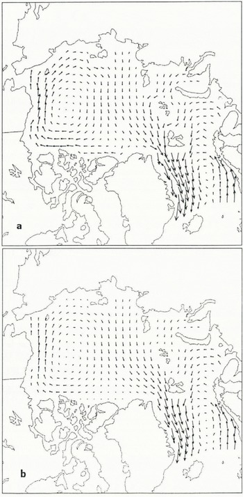
Fig. 2. Annual average ice-velocity field for the third year of the simulations with daily varying wind forcing and 1 d time steps: (a) Cavitating-fluid correction with linear wind and water drag; (b) Viscous-plastic model with quadratic wind and water drag. A velocity vector one grid cell long is approximately 0.08 m s−1.
to the standard viscous-plastic model (Hibler, Reference Hibler1979) which uses non-linear drag for both wind and water and has a shear strength which is one-half the compressive strength. The models were run for three years repeating the one-year forcing described above, both with daily varying and monthly average wind forcing for the dynamic part of the models. In all cases daily forcing and 1 d time steps were used in the thermodynamic part of the models. 1 d time steps were used in the dynamic part of both models except for the monthly average wind cavitating-fluid case which used 5 d time steps for added computational speed. It might be noted here that the cavitating-fluid scheme requires about half the computational effort of the viscous-plastic model for both the daily varying and monthly average wind cases. The cavitating-fluid scheme would be less efficient in the monthly average wind case if 1 d time steps were used; however it has other advantages which will be described shortly.
The third-year average annual velocity fields in Figure 2 illustrate the similarity in mean circulation patterns and magnitude between the two models. It would thus appear that, although the cavitating-fluid correction exhibits a slightly more robust circulation, over a yearly cycle both models will produce similar lateral heat and salt fluxes. The monthly average velocities over the Arctic basin, shown in Figure 3, allow a more detailed comparison between the two models. During the summer months the ice is relatively thin and disperse and so both models produce very similar results (essentially free drift in both cases). During the winter, however, the cavitating-fluid model produces consistently larger velocities due to the lack of shear strength. The absence of shear resistance in the cavitating-fluid correction proves advantageous in the case of monthly average forcing as a relatively robust circulation is maintained; the viscous-plastic model exhibits almost no motion during the winter in this case.
The March thickness contours for the third year of the daily forcing case are shown in Figure 4. Both models produce thickness patterns which are grossly similar, particularly when compared to the thermodynamics-only model (not shown) for which the thickness is a maximum near the pole and decreases radially outward. The slightly more robust circulation in the cavitating-fluid model (Fig. 4a) produces a clockwise shift in the thickness pattern compared to the viscous-plastic model (Fig. 4b). The thickness build-up north of Greenland exhibited by the viscous-plastic model is due to “arching” across Fram Strait inhibiting outflow from the basin. The lack of shear strength in the cavitating-fluid model removes this restriction and, in fact, if linear drag is used for both models, this effect leads to slightly larger outflow for the cavitating-fluid model. In the present case however, the increased force due to non-linear wind drag offsets the outflow restriction and leads to a somewhat larger net outflow for the viscous-plastic model.

Fig. 3. Monthly average velocity magnitude in Arctic basin for the third year of the simulations using daily varying and monthly average wind forcing. VP indicates viscous-plastic model. CF indicates cavitating-fluid correction.
The monthly average basin outflows for the various models are compared in Figure 5. The total annual basin outflows are: viscous-plastic daily wind, 2880 km3; cavitating-fluid daily wind, 2080 km3; viscous-plastic monthly average wind, 1660 km3; cavitating-fluid monthly average wind, 2100 km3. As in the comparison of the basin average velocities, the cavitating-fluid model is much less affected by smoothing of the wind field.
The thickness fields in Figure 4 allow a comparison of the spatial distribution of ice calculated by the two models; on the other hand, seasonal variation is illustrated by the time series of ice volume in the Arctic basin shown in Figure 6. These time series and the basin outflows discussed above further reveal the differences between the models, and more important, demonstrate the important feed-back between dynamics and thermodynamics. The first point to note is that, for daily forcing, the viscous-plastic model retains somewhat more ice in the basin than the cavitating-fluid model in spite of its greater outflow. This is due primarily to the increased thickness build-up by ridging and the concomitant ice growth as leads are opened up: a result of the greater forces generated by quadratic wind drag.

Fig. 4. Thickness fields at the end of March of the third year of the simulations using daily varying wind forcing and 1 d time steps: (a) Cavitating-fluid correction; (b) Viscous-plastic model. Contour interval is 0.25 m.

Fig. 5. Monthly average outflow of ice from the Arctic basin for the third year of the simulations using daily varying and monthly average wind forcing. VP indicates viscous-plastic model. CF indicates cavitating-fluid correction.
For the smoother monthly average forcing, both models have almost identical ice volumes. In this case the forces are insufficient to produce large thickness build-up in either model and the difference in outflow is made up by the increased open-water production associated with more robust circulation in the cavitating-fluid model. The upper curve in Figure 6 shows the excessive ice volume calculated by a thermodynamics-only model in which there is no ice motion and hence no outflow or creation of open water by divergence (this model was run for six years as it is slower to reach equilibrium). It is interesting to note that, although the magnitude of the circulation is less in the monthly average forcing case, the basin ice volume is lower than the daily forcing case. The main reason for this apparent contradiction is the rather subtle reduction in open-water production and hence overall ice production accompanying the less robust monthly average forcing combined with the maintenance of a reasonable ice outflow from the basin. This further emphasizes the importance of dynamic processes in that the result of changing wind forcing may be

Fig. 6. Time series of ice volume (in km3) in the Arctic basin for the third year of the simulations (except for the thermodynamics-only model which was run for six years, since it is slower to reach a seasonal equilibrium): (1) Thermodynamics-only; (2) Viscous-plastic, daily wind forcing; (3) Cavitating fluid, daily wind forcing; (4) Viscous-plastic, monthly average wind forcing; (5) Cavitating-fluid, monthly average wind forcing and 5 d time steps.
counter-intuitive. In the above example, slower ice motion due to smoother wind forcing led to ice-growth (and hence atmospheric heat flux) conditions much less like the no-motion case of thermodynamics-only than one might have expected.
Conclusions
Sea-ice dynamics and its coupling to thermodynamics should not be ignored even in crude-resolution climate studies. We have shown that a very simple approximation to a cavitating fluid provides ice velocity and thickness build-up results which compare favourably in their large-scale features with the more complete Hibler (Reference Hibler1979) viscous-plastic model and represents a significant improvement over thermodynamics only. With daily varying wind, this cavitating-fluid correction scheme runs about twice as fast as the standard viscous-plastic model and is very easy to implement. For smoothed (monthly averaged) wind fields, the cavitating-fluid correction is no more efficient than the viscous-plastic model; however, it has the advantage that it maintains a robust and realistic circulation pattern. It should be emphasized that the lack of shear strength in the cavitating-fluid model does affect the details of the thickness and circulation patterns and so is more appropriate for long-term, crude-resolution climate studies than for the predictions of ice drift and local build-up. Overall, we feel the simple velocity correction scheme presented here is preferable to other ad hoc schemes as an iterative correction to a given ice-velocity field, and is particularly useful when a model is to be forced by smoothed wind fields.
Acknowledgements
This work was funded by the U.S. Office of Naval Research, contract number N00014-86-K-069. The vector and contour plots were produced using NCAR graphics with the help of J. Waugh.
Appendix A
Averaging the velocities on each face of the grid cell for notational simplicity (and denoting each face as I, r, t, b for left, right, top, and bottom, respectively), the velocity corrections of Equation (8) are applied to these velocities such that, after correction, the sum of the velocities squared (a measure of the energy) is:
whereas before correction:
Substituting Equation (A2) into Equation (Al) and noting that the divergence, D, is:

we get, after some algebra, that:

Since all of the terms in Equation (A3) are positive definite, the sum of the velocities squared has decreased while the momentum averaged over the grid cells remains approximately the same. In other words, the energy of the system is decreased by recursive application of the correction scheme but the momentum remains the same; the scheme must therefore converge to a solution. That the solution is unique is guaranteed by the fact that it satisfies both the governing differential equation and the boundary conditions.


