


1. Introduction
Emulsions are multiphase flows of two immiscible (totally or partially) liquid phases with similar densities. Such flows are extremely common in industrial applications such as pharmaceuticals (Nielloud Reference Nielloud2000; Spernath & Aserin Reference Spernath and Aserin2006), food processing (McClements Reference McClements2015), oil production (Kokal Reference Kokal2005; Mandal et al. Reference Mandal, Samanta, Bera and Ojha2010; Kilpatrick Reference Kilpatrick2012) and waste treatment. Emulsions are also relevant for environmental flows such as oil spilling in oceans, when the oil droplets distribution becomes fundamental for quantifying environmental damage (Li & Garrett Reference Li and Garrett1998; French-McCay Reference French-McCay2004; Gopalan & Katz Reference Gopalan and Katz2010). Many studies have been performed on the rheological behaviour of emulsions in the past (Einstein Reference Einstein1906, Reference Einstein1911; Jansen, Agterof & Mellema Reference Jansen, Agterof and Mellema2001; Pal Reference Pal2000, Reference Pal2001; De Vita et al. Reference De Vita, Rosti, Caserta and Brandt2019), while the current knowledge on their behaviour in turbulent flows is limited (Yi, Toschi & Sun Reference Yi, Toschi and Sun2021).
The two fluids are usually referred to as continuous phase (or carrier phase in case of strong advection) and dispersed phase (or droplet phase) depending on whether the volume fraction  $\alpha$ is respectively greater or lower than $0.5$; the system is denoted as binary flow when $\alpha = 0.5$. As the density ratio is usually considered to be close to 1, gravity effects are negligible with respect to the stirring and advection needed to sustain turbulence in the flow. For this reason, four dimensionless numbers can be used to describe these flows, namely the Reynolds number $Re$, the Weber number $We$, the volume fraction of the dispersed phase, and the viscosity contrast. Depending on the specific configuration under investigation, the definitions of these numbers can change, yet they completely define the case studied provided that the two fluid have the same density.
Several aspects of fundamental importance in emulsions, such as turbulence modulation, droplet size distributions and interphase energy fluxes, are not fully understood. We therefore aim to partially fill this gap by means of numerical simulations. In the following, we provide an overview of the main results available in the literature. Results for bubble/droplet-laden flows are also discussed when relevant to the present work.
1.1. Observations on droplet size distribution
The droplet size distribution (DSD) is a key aspect of emulsions, as its prediction becomes fundamental in most applications. In his early seminal work, Kolmogorov (Reference Kolmogorov1949) discussed the criteria under which a droplet undergoes breakup when subject to surrounding turbulence. Kolmogorov first proposed a dimensional argument according to which surface tension forces need to be balanced locally by turbulent energy fluctuations. This idea was later addressed in Hinze (Reference Hinze1955) and translated into a critical Weber number  $We_c$ of order 1 at which breakup occurs, leading to the definition of the Hinze scale $d_H$ as the minimum droplet diameter at which breakup may occur due to pressure fluctuations. A general definition for this scale is
 \begin{equation} d_H = \left(\frac{We_c}{2}\right)^{3/5} \left(\frac{\sigma}{\rho_c}\right)^{3/5}\varepsilon^{{-}2/5}, \end{equation}
where  $\sigma$ is the surface tension coefficient, $\rho _c$ is the carrier phase density and $\varepsilon$ is the energy dissipation rate. This estimate proved valid for bubbles (Chan et al. Reference Chan, Johnson, Moin and Urzay2021; Masuk, Salibindla & Ni Reference Masuk, Salibindla and Ni2021) and emulsions (Perlekar et al. Reference Perlekar, Biferale, Sbragaglia, Srivastava and Toschi2012; Mukherjee et al. Reference Mukherjee, Safdari, Shardt, Kenjereš and Van Den Akker2019; Rosti et al. Reference Rosti, Ge, Jain, Dodd and Brandt2020; Yi et al. Reference Yi, Toschi and Sun2021). Different ${O}(1)$ values have been reported for $We_c$ in numerical (Rivière et al. Reference Rivière, Mostert, Perrard and Deike2021) and experimental works (Deane & Stokes Reference Deane and Stokes2002; Lemenand et al. Reference Lemenand, Valle, Dupont and Peerhossaini2017), from $0.5$ up to $5$; for dilute emulsions in turbulence $We_c\approx 1.17$, according to the values from both numerical (Perlekar et al. Reference Perlekar, Biferale, Sbragaglia, Srivastava and Toschi2012) and experimental (Yi et al. Reference Yi, Toschi and Sun2021) data.
For bubbles larger than the Hinze scale, Garrett, Li & Farmer (Reference Garrett, Li and Farmer2000) found that in isotropic turbulent conditions, droplets break with a cascade process, and the diameter distribution follows a  $d^{-10/3}$ power law. This deterministic process can describe accurately bubble size distributions in breaking waves obtained in experiments (Garrett et al. Reference Garrett, Li and Farmer2000; Deane & Stokes Reference Deane and Stokes2002; Qi, Mohammad Masuk & Ni Reference Qi, Mohammad Masuk and Ni2020) and numerical simulations (Deike, Melville & Popinet Reference Deike, Melville and Popinet2016; Chan et al. Reference Chan, Johnson, Moin and Urzay2021). The same power law has also been proposed for emulsions, based on diffuse-interface numerical simulations (Skartlien, Sollum & Schumann Reference Skartlien, Sollum and Schumann2013; Mukherjee et al. Reference Mukherjee, Safdari, Shardt, Kenjereš and Van Den Akker2019; Soligo, Roccon & Soldati Reference Soligo, Roccon and Soldati2019). For bubbles smaller than the Hinze scale, Deane & Stokes (Reference Deane and Stokes2002) suggested the existence of a fragmentation process; in this case, a $d^{-3/2}$ power law is used to fit experimental data accurately. Agreement with this empirical power law has been observed in homogeneous and isotropic turbulence (HIT) for both bubbles (Rivière et al. Reference Rivière, Mostert, Perrard and Deike2021) and emulsions (Mukherjee et al. Reference Mukherjee, Safdari, Shardt, Kenjereš and Van Den Akker2019). The transition between the two power laws is defined by the Hinze scale. A consequence of this transition is that droplets with $d\gg d_H$ generate both local and non-local bubble/droplet production, as they can fragment in droplets both larger and smaller than the Hinze scale (Rivière et al. Reference Rivière, Mostert, Perrard and Deike2021). Although both power laws have been derived under the hypothesis of dilute conditions ( $\alpha \lesssim 0.05$), they have been observed recently in HIT studies of dense emulsions (Mukherjee et al. Reference Mukherjee, Safdari, Shardt, Kenjereš and Van Den Akker2019), raising the question on the effective role of coalescence in the process.
The connection between bubbles and emulsions is non-trivial and deserves special attention. Hinze (Reference Hinze1955) discussed how  $We_c$ depends on the fluid properties of the dispersed phase. He assumed that $We_c=C[1-f(N_{Vi})]$, with $f$ a generic function of the viscosity group $N_{Vi}=\mu _d/\sqrt {\rho _d\sigma d}$, where $\mu _d$ is the dispersed phase viscosity. On the other hand, $d_H$ was derived under the assumption of a dilute emulsion, hence the density in (1.1) refers to the carrier phase, as the phase where the energy dissipation rate $\varepsilon$ could be measured in experiments. This allows the direct application of the Hinze criteria in flows where density/viscosity ratios are significant as in air–water flows. However, significant uncertainties are discussed in the literature about the properties of the function $f$, and the role of the dispersed phase properties remains mostly unknown (Masuk et al. Reference Masuk, Salibindla and Ni2021). Also unknown is the role of turbulence inhomogeneity and anisotropy, which, according to Hinze (Reference Hinze1955), may be a further source of nonlinear effects in the determination of $We_c$. In fact, in flows where the energy dissipation rate shows strong spatial variations, $We_c$ varies for each bubble/droplet, and it assumes meaning only in an average sense, making it difficult to disentangle the effects of turbulence anisotropy and property contrast. Despite all these uncertainties, correlations from Hinze (Reference Hinze1955), Garrett et al. (Reference Garrett, Li and Farmer2000) and Deane & Stokes (Reference Deane and Stokes2002), derived for isotropic turbulent conditions, apply in most studies with strong property contrasts and large-scale anisotropy. This is likely due to the underlying assumption that the breakup process is purely inertial, as it depends only on $\varepsilon$ (Garrett et al. Reference Garrett, Li and Farmer2000). Thus bubble breakup studies become relevant also for the present study.
Finally, it is worth noticing that the flow configuration appears to have a significant impact on DSD, and experimental observations in shear flows can depart quite substantially from the discussed power-law behaviours. The recent work of Yi et al. (Reference Yi, Toschi and Sun2021) presents strong experimental evidences of gamma/log-normal DSD in Taylor–Couette flow, confirming the previous findings of Pacek, Man & Nienow (Reference Pacek, Man and Nienow1998). These configurations are characterized by strong anisotropy, making the comparison with data obtained for emulsions and bubbles in HIT difficult. On the other hand, Soligo et al. (Reference Soligo, Roccon and Soldati2019) studied breakup and coalescence of emulsions dynamic in a turbulent channel flow. These authors observed the appearance of the  $-10/3$ power law for the DSD in the presence of surfactants. It is interesting to observe that in this numerical study, the scaling from Garrett et al. (Reference Garrett, Li and Farmer2000) seems to apply in anisotropic configurations. Fortunately, there has been a significant effort in recreating local HIT conditions in experiments in recent years (Debue et al. Reference Debue, Shukla, Kuzzay, Faranda, Saw, Daviaud and Dubrulle2018; Dubrulle Reference Dubrulle2019; Knutsen et al. Reference Knutsen, Baj, Lawson, Bodenschatz, Dawson and Worth2020), and new studies are expected to provide new insights on these aspects.
1.2. Studies of two-fluid turbulence
With the advent of more powerful computational resources, a significant number of studies have considered droplets in turbulent flows, yet almost all only through diffuse-interface methods that may display significant mass loss. In their study of emulsions in HIT turbulence, Perlekar et al. (Reference Perlekar, Biferale, Sbragaglia, Srivastava and Toschi2012) show that a statistical stationary state can be reached for the DSD. In the study, the authors used the pseudo-potential lattice Boltzmann method (Biferale et al. Reference Biferale, Perlekar, Sbragaglia, Srivastava and Toschi2011), which compensates mass losses (due to droplets dissolution) by artificially re-inflating existing ones. Simulations of the Cahn–Hilliard–Navier–Stokes formulation are presented in Perlekar et al. (Reference Perlekar, Benzi, Clercx, Nelson and Toschi2014) for binary fluids. These authors found that enforcing large-scale HIT arrests coarsening. This result is particularly significant for emulsions (of which binary fluids represent a special case) as it shows that turbulence is the main factor to determine the droplet size. Furthermore, these authors report modified energy spectra for the mixtures, with a crossover in correspondence to the Hinze scale.
Komrakova, Eskin & Derksen (Reference Komrakova, Eskin and Derksen2015) used a free-energy lattice Boltzmann method to simulate numerically emulsion breakup in HIT, induced by an external large-scale linear forcing. Their findings show that energy spectra present deviations with respect to the single-phase configuration and that the numerical method employed may alter the small-scale dynamics of the flow. Finally, increased coalescence is found for volume fractions  $\alpha >0.05$ also owing to the nature of the diffuse-interface method.
Droplet interactions with turbulence have been studied by Dodd & Ferrante (Reference Dodd and Ferrante2016) in decaying isotropic turbulence. Amongst several observations, these authors discuss the effects of droplet breakup and coalescence on the turbulent kinetic energy budget. Droplet coalescence lowers the total amount of area, hence decreases the surface energy and consequently increases the kinetic energy locally, while the opposite occurs in the case of breakup. More recently, Mukherjee et al. (Reference Mukherjee, Safdari, Shardt, Kenjereš and Van Den Akker2019) have studied emulsions in HIT conditions using a pseudo-potential lattice Boltzmann method, discussing droplet statistics and their correlation with the surrounding turbulence. They confirm the findings of Perlekar et al. (Reference Perlekar, Benzi, Clercx, Nelson and Toschi2014) for energy spectra pivoting at the Hinze scale, demonstrating that energy is subtracted from large scales and injected at small scales, while no direct observation of the underlying mechanism is presented. These authors also show that the droplet generation can be described through the Weber number spectra. In the same work, Mukherjee and co-workers discuss and demonstrate the need for using a forcing scale smaller than the turbulent-box size in order to achieve a polydisperse droplet distribution. It is important to note that Mukherjee et al. (Reference Mukherjee, Safdari, Shardt, Kenjereš and Van Den Akker2019) used a pseudo-potential lattice Boltzmann method, which leads to a significant loss of the dispersed mass during the simulation, as discussed fairly by the authors.
As concerns binary fluids, Perlekar (Reference Perlekar2019) shows how the presence of interfaces leads to a different energy transfer mechanism, confirming the conclusions in Dodd & Ferrante (Reference Dodd and Ferrante2016). Perlekar (Reference Perlekar2019) uses the scale-by-scale (SBS) energy balance to show that the energy absorption at larger scales is given mainly by the interface source term in the Cahn–Hilliard equation used by the author to describe the multiphase nature of the flow. Furthermore, Perlekar (Reference Perlekar2019) shows that small-scale statistics are almost unchanged when changing  $We$, while they are affected by the Reynolds number. This study complements the previous findings in binary fluids (Perlekar et al. Reference Perlekar, Benzi, Clercx, Nelson and Toschi2014; Perlekar, Pal & Pandit Reference Perlekar, Pal and Pandit2017), where coarsening was analysed in three- and two-dimensional turbulence by means of a spinoidal decomposition. Rosti et al. (Reference Rosti, Ge, Jain, Dodd and Brandt2020) study droplets in homogeneous shear turbulence, focusing on the effect of the droplet initial diameter and the shear rate magnitude; the results show that a statistically stationary regime (i.e. balance of coalescence and breakup events, and energy balance convergence) can be reached, while the Taylor-scale Reynolds number $Re_\lambda$ decreases with increasing surface tension.
Despite the growing literature on the subject, many issues are yet to be fully understood. In particular, most of the studies have been carried out using diffuse-interface approaches, which cannot exactly represent the surface terms effects yet are key in many situations. In this sense, our work complements the very recent one by Rivière et al. (Reference Rivière, Mostert, Perrard and Deike2021), focused on the bubble breakup dynamics.
1.3. Objectives of the present study
In the present work, we use direct numerical simulations (DNS) to study the effects of viscosity ratio, volume fraction and surface tension on the emulsion turbulent behaviour. The chosen set-up is tri-periodic HIT, with turbulence sustained throughout the simulation time. The analysis is performed at  $Re_\lambda \approx 137$, which is larger than that attained in previous interface-resolved numerical studies of multiphase turbulent flows. Also, volume fraction, viscosity ratio and surface tension are varied to cover most relevant applications (Jansen et al. Reference Jansen, Agterof and Mellema2001). We analyse the turbulence through global and phase-averaged energy balance, energy spectra, SBS energy budget, and probability density functions (p.d.f.s) for the intermittency analysis. Furthermore, we discuss DSD for all cases. In summary, we will show that: (i) the energy balance is significantly altered by the properties of the dispersed phase; (ii) surface tension forces induce an additional mechanism for energy transfer from larger scale towards the energy dissipation range; (iii) the modified energy transport mechanism alters the energy spectra; (iv) the presence of the interface increases intermittency and alters the small-scale statistics; (v) the DSD displays both the $d^{-3/2}$ and $d^{-10/3}$ power laws, with remarkable accuracy also for $d< d_H$.
2. Methodology
2.1. Governing equations and numerical method
We consider an incompressible flow obeying the continuity and Navier–Stokes equations
 \begin{gather} \partial_i u_i = 0, \end{gather}
 \begin{gather}\rho(\partial_t u_i+u_j\,\partial_j u_i) ={-}\partial_i p + \partial_i \left[ \mu (\partial_i u_j + \partial_j u_i) \right] +f^\sigma_i +f^T_i , \end{gather}
where  $u_i$ is the velocity in the $i$th direction, $p$ is the pressure, and $\rho$ and $\mu$ are the local density and viscosity. The forcing term $f^\sigma _i = \sigma \xi \delta _s n_i$ represents the surface tension force, where $\sigma$ is the surface tension, $\xi$ is the local interface curvature, $n_i$ is the $i$th component of the surface normal vector, and $\delta _s$ the Dirac delta function that ensures that the surface force is applied only at the interface (Tryggvason, Scardovelli & Zaleski Reference Tryggvason, Scardovelli and Zaleski2011). The last term in (2.1b) is the forcing needed to sustain turbulence by injecting energy at the large scales; among the several algorithms available to force sustained homogeneous and isotropic turbulence (e.g. Eswaran & Pope Reference Eswaran and Pope1988; Rosales & Meneveau Reference Rosales and Meneveau2005; Mallouppas, George & van Wachem Reference Mallouppas, George and van Wachem2013; Bassenne et al. Reference Bassenne, Urzay, Park and Moin2016), we use here the Arnold–Beltrami–Childress (ABC) forcing (Mininni, Alexakis & Pouquet Reference Mininni, Alexakis and Pouquet2006)
 \begin{equation} \left.\begin{gathered} f^T_x = A \sin \kappa_0 z + C\cos \kappa_0 y, \\ f^T_y = B\sin \kappa_0 x + A\cos \kappa_0 z, \\ f^T_z = C\sin \kappa_0 y + B\cos \kappa_0 x, \end{gathered}\right\} \end{equation}
with  $x,y,z\in [0,2{\rm \pi} ]$. As reported by Podvigina & Pouquet (Reference Podvigina and Pouquet1994), the ABC forcing creates an unstable single-phase flow for $1/\nu >20$, with $\nu$ the kinematic viscosity and $\kappa _0$ the forcing wavelength.
The description of the code and the algorithm used can be found in Rosti, De Vita & Brandt (Reference Rosti, De Vita and Brandt2019) and Rosti et al. (Reference Rosti, Ge, Jain, Dodd and Brandt2020), together with several validations. The method is therefore described only briefly here; see also Costa (Reference Costa2018) for references to the code structure. The equations are discretized on a staggered uniform Cartesian mesh; the spatial derivatives are computed using second-order centred finite differences, and a second-order Adam–Bashford scheme is used for the time integration. The pressure splitting method presented in Dodd & Ferrante (Reference Dodd and Ferrante2014) is used to obtain a constant-coefficient Poisson equation, which we then solve with the direct fast Fourier transform based pressure solver presented in Costa (Reference Costa2018).
The interface between the two fluids is described with the volume of fluid (VOF) method, in particular the Multi-dimensional Tangent Hyperbola Interface Capturing (MTHINC) algorithm developed by Ii et al. (Reference Ii, Sugiyama, Takeuchi, Takagi, Matsumoto and Xiao2012). The advection equation for the VOF can be written in divergence form as
 \begin{equation} \partial_t \phi + \partial_i u_i\,\mathcal{H} = \phi\,\partial_i u_i, \end{equation}
where  $\mathcal {H}$ is the colour function assuming the values 0 and 1 in each of the fluids, and $\phi$ is the cell-averaged value of $\mathcal {H}$. In the MTHINC method, the function $\mathcal {H}$ is approximated locally using the hyperbolic tangent:
 \begin{equation} \mathcal{H}(x',y',z') \approx \tfrac{1}{2}(1+\tanh(\beta(P(x',y',z')+d))), \end{equation}
where  $(x',y',z')\in [0,1]$ is the cell-centred local coordinate system, $\beta$ is a sharpness parameter (equal to 1 in the current work), $d$ is a normalization factor, and $P$ is the three-dimensional surface function, assumed here to be quadratic (Ii et al. Reference Ii, Sugiyama, Takeuchi, Takagi, Matsumoto and Xiao2012). The advantage of the method is that (2.4) allows us to solve the fluxes in (2.3) by semi-analytical integration. Once the VOF function $\phi$ is known, we evaluate the local fluid properties as
 \begin{equation} \left.\begin{gathered} \rho = \rho_d \phi + \rho_c(1-\phi), \\ \mu = \mu_d \phi + \mu_c(1-\phi), \end{gathered}\right\} \end{equation}
where the subscripts  $c$ and $d$ indicate carrier and dispersed phase, respectively. Finally, the continuum surface force (CSF) model is used to compute the surface tension force (Brackbill, Kothe & Zemach Reference Brackbill, Kothe and Zemach1992), with the normal evaluated with Young's method and the curvature as in Ii et al. (Reference Ii, Sugiyama, Takeuchi, Takagi, Matsumoto and Xiao2012).
2.2. Flow configuration
All the simulations are performed using the same ABC forcing, injecting energy at wavenumber  $\kappa _0=2{\rm \pi} /\mathcal {L}=2$, with $A=B=C=1$, corresponding to $Re_\lambda \approx 137$ for the single-phase flow (see Appendix B for the characteristics of the reference single-phase flow). As reported in the literature (Komrakova et al. Reference Komrakova, Eskin and Derksen2015; Mukherjee et al. Reference Mukherjee, Safdari, Shardt, Kenjereš and Van Den Akker2019), forcing the second wavelength is recommended in order to avoid coalescence induced by large turbulent structures in periodic domains.
In addition to the Reynolds number, the emulsion flows are characterized by four non-dimensional parameters: the volume fraction  $\alpha =\mathcal {V}_d/\mathcal {V}$, defined as the ratio between the volume occupied by the dispersed phase $\mathcal {V}_d$ and the total volume $\mathcal {V}=(2{\rm \pi} )^3$; the viscosity ratio $\mu _d/\mu _c$, where the subscripts $d$ and $c$ indicate the dispersed and carrier phases; the Weber number $We_\mathcal {L}=\rho _c\mathcal {L} u_{rms} ^2/\sigma$, where $u_{rms}$ is the space–time average of the root-mean-square velocity of the single-phase case (which can be related to the forcing amplitude $A=B=C$); and the scale of the ABC forcing $\mathcal {L}$. Finally, the density ratio $\rho = \rho _c/\rho _d$ is kept constant, equal to 1 in this study.
Here, we will vary the dispersed phase volume fraction, the viscosity ratio and the Weber number; the parameters pertaining to the different simulations discussed below are presented in table 1. A convergence study motivating the choice of the resolution in the table is reported in Appendix B. Finally, the resolution  $N=512$ has been chosen as it allows us to resolve adequately all the different cases. Note, finally, that the table also indicates the integration time $N_\mathcal {T}$ required to reach statistical convergence of the turbulent quantities and DSD in units of large eddy turnover times, $\mathcal {T}=\mathcal {L} u_{rms}$ (Mininni et al. Reference Mininni, Alexakis and Pouquet2006). The simulations are considered at convergence when global energy production balances dissipation (see § 2.3 and (2.7) for their definitions) with an error of less than $4\,\%$, also implying that the average of the time derivative of the interfacial area is negligible (see Appendix B for further details). Interestingly, $N_\mathcal {T}$ varies significantly with the physical configuration. In particular, starting with the reference cases BE1 and BE2, we observe that increasing $\mu _d/\mu _c$ means longer times are needed to reach a statistically stationary state, which we will attribute to a decrease of the breakup rate. A similar behaviour is observed when decreasing $We_\mathcal {L}$, when higher surface tension forces decrease the probability of breakup events. Finally, large structures become unavoidable when increasing the volume fraction $\alpha$ (Komrakova et al. Reference Komrakova, Eskin and Derksen2015; Mukherjee et al. Reference Mukherjee, Safdari, Shardt, Kenjereš and Van Den Akker2019), which implies longer simulation times.
Table 1. Parameter settings for the simulations considered in this study: number of grid points in each direction  $N$, viscosity ratio $\mu _d/\mu _c$, Weber number $We_\mathcal {L}$, with surface tension $\sigma$, volume fraction $\alpha$ and integration time to reach statistical convergence $N_\mathcal {T}$. All simulations are performed with $\mu _c=0.006$ and the same ABC forcing. Each case is denoted by a letter indicating the parameter that is varied: V for viscosity ratio, C for volume fraction, and W for Weber number. SP are the single-phase flows, and BE are configurations that recur in different parametrizations (base emulsions).

Visualizations of the transient phase to reach the final steady state are reported in figure 1 for the reference case BE1 with  $\alpha =0.03$. The simulation starts at $t_0$ using the fully developed single-phase HIT field from case SP2. The dispersed phase is initialized as an ensemble of spheres, which soon deform in the flow as shown in figure 1(b), pertaining to time $t_1=\mathcal {T}/4$. At statistical convergence, $t \approx 10\mathcal {T}$, when statistics are collected, we observe a polydispersed distribution of asymmetric droplets. Note finally that for $\alpha \leqslant 10\,\%$, the simulations are initialized using spherical droplets of size $d_0\approx 0.12L$, while a single spherical droplet of initial size $d_0=(6\alpha L^3/{\rm \pi} )^{1/3}$ was used for larger values of $\alpha$. We have checked that the initial distribution has no effect on the final DSD, as also reported in Mukherjee et al. (Reference Mukherjee, Safdari, Shardt, Kenjereš and Van Den Akker2019) for a similar configuration.

Figure 1. Initial evolution of the emulsion flow (example reported for case BE1). The droplets are initialized at  $t_0$ in a developed turbulent field. As turbulence is maintained, breakup and coalescence start occurring ( $t_1$), and statistical convergence in the DSD is achieved after a few turnover times ( $t_2$): (a) $t_0$, (b) $t_1=\mathcal {T}/4$, (c) $t_{2}=10\mathcal {T}$.
2.3. Observables, phase-averaged energy balance and scale-by-scale budget
In this subsection, we introduce the theoretical tools and the physical observable that will be discussed throughout the study. The full mathematical derivation, as well as details on the computation of the energy spectrum and DSD, can be found in Appendix A. The objective of this study is to understand the turbulence modulations induced by a second phase, focusing on comparisons of the energy spectra and the SBS analysis. In particular, we will consider the Taylor-scale Reynolds number, the energy spectra, the phase-averaged energy balance, p.d.f.s of velocity fluctuations, dissipation and vorticity, and the SBS budgets. The Taylor-scale Reynolds number is defined as
 \begin{equation} Re_\lambda = \left(\frac{u_i u_i}{3}\right)^{1/2} \frac{\lambda}{\nu}, \end{equation}
where  $\lambda =(5\nu u_i u_i/\varepsilon )^{1/2}$ is the Taylor scale, with the energy dissipation rate computed as $\varepsilon =\nu \,\partial _i u_j\,\partial _j u_i$ for the reference single-phase flow $Re_\lambda =137$. Here, we compute $\varepsilon$ and all the relevant observables at each computational grid point and then average in space and time. This procedure is required due to material properties discontinuities when $\mu _d/\mu _c$ is varied. Note that from now on, $\varepsilon$ will denote the space–time averaged value.
Further insight on the global behaviour of multiphase flows can be gained through the phase-averaged energy balance:
 \begin{gather} \rho\,\partial_t k_m = \mathcal{P}_m - \varepsilon_m + \mathcal{T}^\nu_m + \mathcal{T}^p_m, \end{gather}
 \begin{gather}k_m=\langle u_i u_i/2 \rangle_m, \quad \mathcal{P}_m = \rho\langle u_i f^T_i\rangle_m, \quad \varepsilon_m = \langle \nu\,\partial_j u_i\,\partial_i u_j\rangle_m, \end{gather}
 \begin{gather}\mathcal{T}^\nu_m = \langle \partial_j \mu u_i \left(\partial_j u_i + \partial_i u_j\right)\rangle_m, \quad \mathcal{T}^p_m ={-}\langle\partial_i u_i p\rangle_m. \end{gather}
Here,  $\mathcal {P}_m$ and $\varepsilon _m$ indicate, respectively, production rate and viscous dissipation rate per unit volume in each phase. The terms $\mathcal {T}^\nu _m$ and $\mathcal {T}^p_m$ are the viscous and pressure transport densities, respectively, and represent the coupling between the two phases; when the sum of these two, $\mathcal {T}_m = \mathcal {T}^\nu _m +\mathcal {T}^p_m$, is positive, energy is absorbed from phase $m$, when negative energy is transferred to the other phase. Again, in statistical stationary conditions, $\partial _t k_m\approx 0$. Further details on the derivation of (2.7) can be found in Appendix A.
We now move to spectral space and present the SBS balance. This is derived for the two-fluid flows following the formulation in Olivieri et al. (Reference Olivieri, Akoush, Brandt, Rosti and Mazzino2020a,Reference Olivieri, Brandt, Rosti and Mazzinob); for more details, the reader is referred to Frisch (Reference Frisch1995) and Alexakis & Biferale (Reference Alexakis and Biferale2018). Taking the Fourier transform of the momentum equations (2.1b), we obtain
 \begin{equation} \partial_t \tilde{u_i} + \tilde{G}_i = -\mathrm{i}\kappa\widetilde{p/\rho} - \tilde{V}_i + \tilde{f^\sigma_i} +\tilde{f_i^T}. \end{equation}
Denoting the Fourier transform of a quantity  $J(x_i,t)$ as $\tilde {J}(\kappa _i,t)=\mathscr {F}\{J(x_i,t)\}$, with $\kappa _i$ the $i$th component of the wavelength vector, in the expression above we have $\tilde {G}_i = \mathscr {F}\{u_j\,\partial _j u_i\}$ and $\tilde {V}_i = \mathscr {F}\{\partial _i(\nu [\partial _i u_j + \partial _j u_i])\}$. Note that as the viscosity $\mu$ is a function of space and time, we actually compute the dissipation term in physical space to avoid a convolution in the spectral space. We next multiply (2.8) with the complex conjugate of the velocity $\tilde {u}_i^*$, and drop the pressure term by imposing the incompressibility condition $\kappa _i\tilde {u}_i=0$, as in this work $\rho _c=\rho _d=1$. Multiplying the complex conjugate of (2.8) by $\tilde {u}_i$, summing the equations obtained for $\tilde {u}$ and $\tilde {u}^*$, and averaging in time, we finally obtain
 \begin{equation} \partial_t E(\kappa_i) = T(\kappa_i) + \mathcal{D}(\kappa_i) +\mathcal{S}_\sigma(\kappa_i) + \mathcal{F}(\kappa_i), \end{equation}
where
(i) $E = \langle \tilde {u}_i\tilde {u}_i^*\rangle _t$ is the time-averaged kinetic energy in the spectral domain, whose time derivative is zero at statistical steady state;
(ii)
$T = -\langle \tilde {G}_i\tilde {u}_i^* + \tilde {G}_i^*\tilde {u}_i\rangle _t$ is the time-averaged energy transfer due to the nonlinear term;(iii)
$\mathcal {D} = -\langle \tilde {V}_i\tilde {u}_i^* + \tilde {V}_i^*\tilde {u}_i\rangle _t$ is the time-averaged viscous dissipation;(iv)
$\mathcal{S}_\sigma = -\langle\tilde{f_i^\sigma}\tilde{u}_i^* + \tilde{f_i^\sigma}^*\tilde{u}_i\rangle_t$ is the time-averaged work of the surface tension force at the different scales;(v)
$\mathcal{F} = \langle\tilde{f^T_i}\tilde{u}_i^* + \tilde{f^T_i}^*\tilde{u}_i\rangle_t$ is the time-averaged energy input due to the large-scale forcing.


All of the above are three-dimensional fields in spectral space. Note that at steady state when the total interfacial area is constant,  $\mathcal {S}_\sigma$ integrates to zero (Dodd & Ferrante Reference Dodd and Ferrante2016), so this term can be seen effectively as an energy transport due to the surface tension.
Finally, we perform a spherical-shell integral in spectral space and express each term in the budget as a function of the magnitude of the wavevector  $\kappa$. This operation results in e.g.
 \begin{equation} T(\kappa) = \sum_{\kappa<|\kappa_i|<\kappa+1} T(\kappa_i). \end{equation}
This term represents the shell-to-shell energy transfer function for the nonlinear term of the momentum equation, and similarly for the other terms above.
3. Results
3.1. Emulsions at different volume fractions
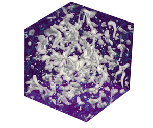
We first examine the influence of the dispersed-phase volume fraction on the turbulent flow, cases BEx and Cxx in table 1, corresponding to increasing values of  $\alpha$ from 3 % to 50 %. A render of the cases discussed here is shown in figure 2, where the iso-contours of VOF fields are shown for volume fractions $0.06$, $0.2$ and $0.5$.

Figure 2. Render of the two-fluid interface (corresponding to the value of the VOF function  $\phi =0.5$) for different values of the volume fraction $\alpha$: (a) $\alpha =0.06$, (b) $\alpha =0.2$, (c) $\alpha =0.5$. The vorticity fields are shown on the box faces on a planar view.
The modulation of the turbulence is first quantified in terms of integral quantities. Figure 3 shows  $Re_\lambda$, computed according to (2.6), versus the volume fraction $\alpha$. Here, $Re_\lambda$ increases almost linearly with $\alpha$, by approximately 15 % for $\alpha =0.5$. A similar trend is found for $\lambda$, as shown in the inset of figure 3. Considering that the average of $\varepsilon$ and $k$ is approximately constant in all cases (variations of ${\pm }3\,\%$), the increase of $Re_\lambda$ and $\lambda$ is therefore due to the local variations of the ratio $k/\varepsilon$.

Figure 3. Taylor-scale Reynolds number  $Re_\lambda$ versus the dispersed-phase volume fraction $\alpha$, for viscosity ratio $\mu =1$ and density ratio $\rho =1$. The inset shows the Taylor scale, $\lambda$, versus the different values of $\alpha$ under investigation.
In particular, the increased values of  $k/\varepsilon$ for similar averaged values of the two quantities is attributed to the increased correlation between regions of strong turbulent kinetic energy and low dissipation. Graphical evidence is presented in figure 4, where we show the instantaneous ratio $k/\varepsilon$ for the single-phase (case SP2 in panel a) and multiphase flows (case BE2 with $\alpha =0.1$ in panel b) in logarithmic scale. The figure shows that when the dispersed phase is present, large regions of fluid with higher $k/\varepsilon$ are observed far from the droplet interface (denoted with a white line). This can be explained as follows: as the total dissipation is constant, the local increase of $\varepsilon$ near the interface, as also observed in Dodd & Ferrante (Reference Dodd and Ferrante2016), corresponds to a decrease of the dissipation rate in large portions of the fluid, those far from an interface. Considering that the turbulent kinetic energy is less affected by the presence of the interface, the ratio $(k/\varepsilon )$ increases in average. To support this statement, figures 4(c,d) depict the instantaneous energy dissipation rates for the same planes. In the emulsion (panel d), higher values of $\varepsilon$ are found close to the droplet interface and to the clustering regions, while for the single-phase flow (panel c), no specific pattern is observed.

Figure 4. (a,b) Contours of the ratio  $k/\varepsilon$ with logarithmic scale in two planes. (c,d) Energy dissipation rate $\varepsilon$. (a,c) Results for the single-phase case SP2. (b,d) Results for case BE2 ( $\alpha =0.1$). The white lines represent the VOF iso-contours for $\phi =0.5$.
The one-dimensional energy spectra  $E(\kappa )$ multiplied by $\kappa ^{5/3}$, i.e. the so-called compensated spectra, are displayed in figure 5 for the different $\alpha$ considered. The Taylor scale of the single-phase flow is indicated by the dot-dashed line, while the vertical dotted black line is used for the wavenumber $\kappa _H$ corresponding to the Hinze scale, defined as
 \begin{equation} d_H = 0.725\varepsilon^{{-}2/5}(\rho_c/\sigma)^{{-}3/5}. \end{equation}
Figure 5. Compensated energy spectra for simulations at different volume fractions  $\alpha$; the dot-dashed line represents Taylor scale $\lambda$, while the dotted line represents the Hinze scale $d_H$.
Note that the prefactor  $0.725$ in (3.1) is set according to the original work of Hinze (Reference Hinze1955) for emulsions in HIT conditions, corresponding to $We_c=1.17$.
The data in figure 5 reveal that the presence of the dispersed phase reduces the energy with respect to the single-phase case (SP1) for  $\kappa <\kappa _H$. At the same time, the energy content increases at the smaller scales, $\kappa >\kappa _H$, in the dissipative range of the spectra. As noted in previous studies (Mukherjee et al. Reference Mukherjee, Safdari, Shardt, Kenjereš and Van Den Akker2019), the amount of energy subtracted to the large scales is proportional to the volume fraction $\alpha$. Interestingly, the wavenumber at which the curves cross over from reduced to increased energy content corresponds to the Hinze scale. For brevity, we will denote as the pivoting point the wavelength where the spectra of the multiphase cases intersect the one from the single-phase reference case.
Pivoting points were not observed clearly in some previous studies on emulsions (Mukherjee et al. Reference Mukherjee, Safdari, Shardt, Kenjereš and Van Den Akker2019; Perlekar Reference Perlekar2019), while they are clearly visible in others (Perlekar et al. Reference Perlekar, Benzi, Clercx, Nelson and Toschi2014; Dodd & Ferrante Reference Dodd and Ferrante2016; Rosti et al. Reference Rosti, Ge, Jain, Dodd and Brandt2020). This is possibly due to the different methods used to simulate the dispersed phase: the ability of the VOF to accurately resolve the interface reduces the energy dissipation by the surface tension term in the dissipative range. Such energy dissipation is indeed observed clearly by Perlekar (Reference Perlekar2019), who present results obtained by solving the Cahn–Hilliard equation in a diffuse-interface formulation. As mentioned in Appendix B, these numerical artefacts do not have significant effects on the dynamics at the inertial range, while they affect the dissipative range. This aspect will also be discussed later in this section.
Insight into the energy transfer among the different scales is gained by using the SBS analysis. The full SBS energy budget, i.e. the contributions from the different terms in (2.9), is displayed in figure 6(a) for case BE2, chosen as an illustrative example with an intermediate value  $\alpha =0.1$. The external forcing is injecting energy at $\kappa =2$, which is absorbed by the nonlinear transfer term $T$ for a large majority, and by the surface tension term $\mathcal {S}_\sigma$ for a small part. The nonlinear term transfers energy towards smaller scales, larger values of $\kappa$. The surface tension term, $\mathcal {S}_\sigma$, acts as a dissipative process at large scales, where it absorbs approximately the same energy as the dissipative term $\mathcal {D}$. However, for $10<\kappa <20$, we observe a significant change in the energy transport mechanism: $\mathcal {S}_\sigma$ becomes positive, hence contributing to transferring energy towards the small scales, similarly to $T$, a process active until $\kappa _{max}$. It is important to note that the surface tension transport remains active also at small scales in the dissipative range, consequently extending the range of wavelengths where the dissipation term remains active. These observations confirm the previous findings obtained in Perlekar (Reference Perlekar2019) for binary mixtures, while showing that dissipation at small scales is due only to $\mathcal {D}$ in the case of sharp interface methods.

Figure 6. Scale-by-scale energy budget for different volume fractions  $\alpha$. (a) Full energy balance for the case BE2 with $\alpha =0.1$; (b) the energy transfer $T$ due to the nonlinear terms; (c) the energy transfer $\mathcal {S}_\sigma$ associated with the surface tension term; (d) energy dissipation rate $\mathcal {D}$.
The details of the effect of the volume fraction  $\alpha$ on each term of the SBS balance are displayed in figures 6(b–d). We first analyse the nonlinear transfer term $T$ in panel (b). As $\alpha$ increases, $T$ absorbs progressively less energy at the injection frequency $\kappa =2$. Consequently, less energy is transferred towards smaller scales by nonlinear advection. The energy flux $\varPi$ (not shown) does not display an inverse cascade for any $\alpha$. Furthermore, we notice that no energy is transferred to the far end of the dissipative range, which is resolved over a large range of scales in all cases.
The contribution from the surface tension  $\mathcal {S}_\sigma$ (see figure 6c) confirms that interfacial stresses absorb part of the energy injected into the domain at $\kappa =2$. The energy absorbed by the surface tension term at large scales is approximately proportional to $\alpha$. The surface tension term becomes positive at smaller scales, where energy is released. The positive peak is reached at approximately the Hinze scale for all cases. As for the energy absorption, the magnitude of the peak scales proportionally to $\alpha$. We also notice that for any $\alpha$, the surface tension terms act also in the dissipative range, where the nonlinear term $T$ is zero.
The behaviour observed so far for  $T$ and $\mathcal {S}_\sigma$ provides a clear explanation for the previous observations on the energy spectra. At small wavenumber, the energy cascade produced by the nonlinear energy transfer is partially inhibited by the presence of the interfacial forces. For high wavenumbers, $T$ reaches zero progressively, but the energy previously subtracted by the interfacial stresses at large scale is redistributed at small scales, which can be seen in figure 5 as an energy increase at high wavenumbers.
To close the SBS balance, we examine the viscous dissipation term  $\mathcal {D}$ (see figure 6d). First, we note that only a small amount of the injected energy (less than $5\,\%$ for all cases) is absorbed by the dissipation term at the scale of the forcing, $\kappa = 2$. The overall effect of the dispersed phase is to shift the energy dissipation towards smaller scales. This constitutes the natural reaction of the system to the increased activity in the dissipative range caused by the surface tension term. This behaviour becomes more evident as $\alpha$ increases and progressively enhances dissipation at those small scales where the single-phase dissipation is negligible.
Summarizing, the surface tension introduces an alternative path for energy transmission from large towards small scales, as discussed for binary flows in Perlekar (Reference Perlekar2019). The amount of energy transferred by the surface tension is directly proportional to the total droplets surface area  $\mathcal {A}$, as shown in figure 7(a), where we display the maximum energy transferred via surface tension, $\max (\sum _{|\kappa _i|<\kappa } \mathcal {S}_\sigma (\kappa ))$, and the total area of the dispersed phase $\mathcal {A}$ for the different volume fractions under consideration with a linear fit to the data. This observation reinforces our previous conclusion that the interface transfers energy among different scales by disrupting larger turbulent structures and creating smaller ones, hence affecting the canonical $-5/3$ slope of the turbulence spectra. Note also that while in monodispersed flows this results in a deviation at a specific spectral frequency (Dodd & Ferrante Reference Dodd and Ferrante2016), in polydispersed flows this behaviour is seen at all scales.

Figure 7. (a) Correlation between the maximum surface tension term,  $\max (\sum _{|\kappa _i|<\kappa } \mathcal {S}_\sigma (\kappa ))$, and the total surface area $\mathcal {A}$ for the different volume fractions $\alpha$. The dashed black line is the linear fit to the data. (b) P.d.f. of the DSD for different values of $\alpha$. The dashed black line indicates the $d^{-3/2}$ law from Deane & Stokes (Reference Deane and Stokes2002), the continuous black line the $d^{-10/3}$ law from Garrett et al. (Reference Garrett, Li and Farmer2000), and the dotted black line the Hinze scale $d_H$. The droplet size is normalized by the Kolmogorov scale of simulation SP2, $\eta _{sp}$.
We next consider the dynamics of the dispersed phase. We first examine the DSD for all the values of volume fraction studied – see figure 7(b), where we display the droplet diameters normalized by the single-phase (SP1) Kolmogorov scale  $\eta _{sp}$ . The dashed black line depicts the $d^{-3/2}$ law by Deane & Stokes (Reference Deane and Stokes2002), and the solid line depicts the $d^{-10/3}$ law by Garrett et al. (Reference Garrett, Li and Farmer2000), valid for larger droplets. For small droplets, the $-3/2$ law is well captured also for marginally resolved droplets (with $d/\eta _{sp}<6$). For droplets larger than the Hinze scale, the $-10/3$ law is also a very good fit, with increasing accuracy for increasing values of $\alpha$. Our data are in agreement with the findings by Mukherjee et al. (Reference Mukherjee, Safdari, Shardt, Kenjereš and Van Den Akker2019) and explained by higher coalescence probability at higher volume fractions, leading to a bigger population of larger droplets. Interestingly, the Hinze scale turns out to define approximately the transition between the $-3/2$ and $-10/3$ scalings as proposed in Deane & Stokes (Reference Deane and Stokes2002), although for higher values of $\alpha$, the onset of the $d^{-10/3}$ power law occurs at larger diameters. As the droplet distributions can be, to a good approximation, represented by these two laws, it follows that $\mathcal {A}\propto \alpha$, explaining why $\mathcal {A}$, $\mathcal {S}_\sigma$ and $\alpha$ are linearly correlated (see figure 7a).
We now consider the phase-averaged energy budget, introduced in § 2.3. The different terms of (2.7) – production, dissipation and transport by pressure and viscous forces – are shown in figure 8, normalized by the single-phase dissipation. We first observe that the total production and dissipation is
 \begin{equation} \mathcal{P}= \alpha \mathcal{P}_d + (1- \alpha) \mathcal{P}_c \approx\varepsilon\approx 0.95\varepsilon_{sp} \end{equation}
for  $\alpha <0.5$. The energy production density $\mathcal {P}_m$ (green symbols in figure 8a) is higher in the dispersed phase for low volume fractions, while it is comparable to that of the carrier phase for $\alpha >0.1$. The energy dissipation rate per unit volume in the dispersed phase $\varepsilon _d$ (red symbols in figure 8a) is also larger at low volume fractions and decreases monotonically with increasing $\alpha$. The dissipation in the carrier phase, $\varepsilon _c$, also decreases, as it compensates for the energy transport $\mathcal {T}_m$ from the carrier flow towards the dispersed phase. The viscous transport (see blue symbols in figure 8b) is significantly lower than its pressure-induced counterpart, $\mathcal {T}^p_m$, although they exhibit similar behaviours: they first increase until $\alpha =0.1$, and then decrease to reach zero for a binary mixture. Note, again, that the total transport term is zero, i.e. the sum of $\mathcal {T}^p$ and $\mathcal {T}^{\nu }$ from both phases. The case $\alpha =0.5$ deserves a specific mention. In this case, production and dissipation in the two phases are equal, hence the transport term satisfies $\mathcal {T}_m=0$. Intuitively, it is not possible to define unambiguously a carrier and dispersed phase in binary mixtures; while the energy is locally transported from one phase to the other, the global average is zero for both pressure and viscous transfer.

Figure 8. Phase-averaged energy balance versus the dispersed phase volume fraction  $\alpha$; see (2.7). In each plot, coloured triangles represent the dispersed phase ( $m=d$), while circles represent the carrier phase ( $m=c$). Each term is normalized by the single-phase energy dissipation $\varepsilon _{sp}$ computed for case SP2. (a) Energy production $\mathcal {P}_m$ and energy dissipation $\varepsilon _m$; (b) viscous energy transport $\mathcal {T}^\nu _m$ and pressure energy transport $\mathcal {T}^p_m$.
Finally, we analyse the p.d.f.s of velocity fluctuations  $u_n=u/\sigma _u$, vorticity fluctuations $\omega _n=(|\omega _i|-\langle |\omega _i| \rangle )/\sigma _\omega$, and energy dissipation $\varepsilon _n=(\varepsilon -\langle \varepsilon \rangle )/\sigma _\varepsilon$, normalized by their standard deviations. In figure 9(a), we observe that while the p.d.f. of the velocity fluctuation remains symmetric, the tails deviate strongly from the typical pseudo-Gaussian behaviour of single-phase turbulence (Sreenivasan & Antonia Reference Sreenivasan and Antonia1997; Jimenez Reference Jimenez2000; Ishihara, Gotoh & Kaneda Reference Ishihara, Gotoh and Kaneda2009). Considering the vorticity in figure 9(b), no deviation is observed in the Gaussian core (as defined in Sreenivasan & Antonia Reference Sreenivasan and Antonia1997). However, the distributions of the multiphase flows depart strongly from the single-phase case in the tails. In particular, the exponentially decaying tails have a higher exponent in the case of emulsions, indicating more events with strong vorticity. Interestingly, while increasing the volume fraction does not influence the value of the exponent, increasing $\alpha$ induces deviations in the distributions already at lower values of $\omega _n$. We observe a similar behaviour for $\varepsilon _n$ in figure 9(c): the intermittency of the single-phase flow is amplified by the presence of the interface. As for the vorticity, departures from the single-phase distributions are observed at lower values of $\varepsilon$ when increasing the volume fraction $\alpha$. As a final general remark, the analysis of the p.d.f.s reveals that strong deviations are induced by the presence of the interface, already at low volume fractions, overall increasing the intermittent behaviour of the flow. As no collapse is observed for the normalized variables, it can be inferred that the small-scale statistics are affected by the presence of the interface.

Figure 9. P.d.f.s of (a) velocity fluctuations  $u$, (b) vorticity $\omega$, and (c) dissipation $\varepsilon$. All quantities are normalized as standard score.
3.2. Influence of viscosity ratio
We consider now the influence of the viscosity ratio on the flow turbulence, i.e. cases BEx, V1x and V2x in table 1. The viscosity ratios analysed span the range  $0.01<\mu _d/\mu _c<100$, while $We_\mathcal {L}=42.7$ for all cases. Two values of the volume fractions are considered, $\alpha =0.03$ (series V1x) and $\alpha =0.1$ (series V2x). A render of the two-fluid interface (corresponding to the value of the VOF function $\phi =0.5$) is shown in figures 10(a–c) for cases V11, BE1 and V14, respectively. As $\mu _d/\mu _c$ increases, larger droplets appear; at low viscosity ratios, we find a significantly higher number of droplets.

Figure 10. Render of the two-fluid interface (corresponding to the value of the VOF function  $\phi =0.5$) for different values of the viscosity ratio $\mu _d / \mu _c$: (a) $0.01$, (b) $1$, (c) $100$. The vorticity fields are shown on the box faces on a planar view. All simulations are performed at $\alpha =0.03$ and $We_\mathcal {L}=42.6$.
We start by examining the Taylor-scale Reynolds number of the emulsion flows for the different viscosity ratios under investigation. Figures 11(a) and 11(b) show the variation of  $Re_\lambda$ versus the viscosity ratio for the two volume fractions considered, $\alpha =0.03$ and $\alpha =0.1$. As expected, $Re_\lambda$ decreases with the viscosity ratio. Significant variations in $Re_\lambda$ are observed already for small volume fractions, the effects being amplified for $\alpha =0.1$. In the insets of figure 11, we can observe that $\lambda$ (i.e. the local variations of $k/\varepsilon$) does not increase linearly with $\mu _d/\mu _c$, indicating increased velocity fluctuations for the dispersed phase at lower viscosity.

Figure 11. Taylor-scale Reynolds number of the emulsion flows for the different viscosity ratios examined.  $Re_\lambda$ is shown versus $\mu _d/\mu _c$. (a) Cases BE1 and V1x, with volume fraction $\alpha =0.03$; (b) cases BE2 and V2x, with $\alpha =0.1$. The insets show the evolution of $\lambda$ with the viscosity ratio.
To better quantify the variations of the flow gradients, we show the phase-averaged (see (A2)) enstrophy  $\omega ^2_m$ in figure 12, normalized by the single-phase values from SP1. The viscosity ratio affects enstrophy strongly in the dispersed phase, while the magnitude in the carrier phase is almost constant. Further, smaller variations can be observed when changing the volume fraction from 0.03 to 0.1. For $\mu _d/\mu _c\leqslant 1$, the enstrophy in the dispersed phase goes approximately as $\omega ^2_c\propto -\log (\mu _d/\mu _c)$. As the viscosity of the dispersed phase becomes larger ( $\mu _d>\mu _c$), $\omega _d$ decreases below the average value of the single-phase flow and tends towards zero, as high viscosity dampens velocity fluctuations in the dispersed phase. It is worth noting that for incompressible flows, the energy dissipation rate can be defined as $\varepsilon \equiv \nu |\omega _i|^2$; however, when phase averaging, the two formulations differ for by a term proportional to $\partial _{ii}p$.

Figure 12. Phase-averaged enstrophy  $\omega ^2_m$ (normalized by its value in the single-phase case SP1) for different viscosity ratios $\mu _d/\mu _d$. Triangles indicate the dispersed phase ( $m=d$), while circles indicate the carrier phase ( $m=c$). (a) Results for $\alpha =0.03$; (b) results for $\alpha =0.1$.
We now discuss the influence of viscosity ratio on the compensated energy spectra, shown in figures 13(a,b) for  $\alpha =0.03$ and $\alpha =0.1$, respectively. Similarly to previous observations for figure 5, the Hinze scale shows, to a good approximation, the pivoting point, below which energy increases with respect to the single-phase spectra. Differences in the inertial subrange are hardly observable for $\alpha =0.03$, while they become more prominent when the volume fraction is increased (see figure 13b). Analysis of the data for $\kappa <\kappa _H$ reveals that the simulations with a dispersed phase present less energy than the single-phase case. In the dissipative range, the trend emerges more clearly. As $\kappa >\kappa _H$, the less viscous the dispersed phase, the more energy is injected in the smaller scales. As discussed in the previous section, energy reduces at large scales and increases at small scales when increasing the volume fraction $\alpha$.

Figure 13. One-dimensional compensated energy spectra for (a)  $\alpha =0.03$, and (b) $\alpha =0.1$, and different values of the viscosity ratio $\mu _b/\mu _c$. The vertical dotted line indicates the Hinze scale wavelength, $\kappa _H$.
Figure 14 shows the DSD for all configurations with different viscosity ratios. As for the data in § 3.1, we also display the  $-3/2$ power law, which well describes the distribution of small droplets, and the $d^{-10/3}$ law from Garrett et al. (Reference Garrett, Li and Farmer2000) for larger droplets. In this range, $d>d_H$, the $-10/3$ law is observed only in a limited region of the spectrum. As noted previously, this is most likely due to the low volume fraction considered. The variation of $\mu _d$ has an influence on large droplets, as higher viscosity in the dispersed phase increases the probability of formation of these large droplets. This was also observed qualitatively in figure 10 and confirms previous findings (Roccon et al. Reference Roccon, De Paoli, Zonta and Soldati2017).

Figure 14. P.d.f.s of the DSD for different values of  $\mu$, at (a) $\alpha =0.03$, and (b) $\alpha =0.1$. The dashed line represents the $d^{-3/2}$ scaling from Deane & Stokes (Reference Deane and Stokes2002), while the continuous black line shows the $d^{-10/3}$ law from Garrett et al. (Reference Garrett, Li and Farmer2000).
We present the SBS energy budget for  $\alpha =0.1$ in figure 15. The results for $\alpha =0.03$ show similar trends; see Appendix C for the details. Following the same scheme as in the previous section, we depict in figure 15(a) the energy balance for case V22, when $\mu _b/\mu _c=0.1$. Similarly to previous observations, the dispersed phase absorbs energy at large scales and redistributes it to small scales; that is, the presence of the interface provides an alternative path for energy transfer from small to large wavenumbers and no inverse cascade is observed. The nonlinear energy transfer $T$ (see figure 15b) displays a weak sensitivity to the viscosity ratio (almost negligible for $\alpha =0.03$, as shown in figure 27 in Appendix C). Thus the differences in the $Re_\lambda$ and energy spectra discussed above are not associated with an extension of the inertial range. For wavenumbers larger than that of the forcing, the nonlinear energy transfer is higher at large scales and lower at small scales than for the single-phase case.

Figure 15. Scale-by-scale energy budget for different viscosity ratios  $\mu _d/\mu _c$ at $\alpha =0.1$. (a) Complete energy balance for case V22 with $\mu _d/\mu _c=0.1$; (b) nonlinear energy transfer $T$; (c) the term $\mathcal {S}_\sigma$ associated with the surface tension; and (d) the energy dissipation transfer function $\mathcal {D}$.
Figure 15(c) shows the energy transport due to the surface tension term,  $\mathcal {S}_\sigma$. As $\mu _d/\mu _c$ increases, the wavelength where the positive energy transport is maximum shifts to larger scales. This behaviour is possibly due to increased coalescence for high $\mu _d/\mu _c$ (as discussed later in this section). We also observe that with decreasing viscosity ratio, $\mu _d/\mu _c<1$, the curves tend to collapse, as the data for $\mu _d/\mu _c=0.1$ and $\mu _d/\mu _c=0.01$ are approximately overlapping. At the injection scale, $\kappa =2$, almost all cases behave similarly. At intermediate wavelengths, the lower the viscosity ratio, the higher the energy absorbed by the surface tension forces. As previously observed, the Hinze scale represents, to a good approximation, the point where the energy transfer towards small scales by the surface tension term $\mathcal {S}_\sigma$ is maximum. All these observations apply to the two values of $\alpha$ considered; see also Appendix C.
A note should be made on the flow with the highest viscosity ratio: in this case, the energy is not transferred down to the dissipative range. A qualitative explanation is given by the following scenario. When the interface interacts with a sufficiently large vortex in the carrier phase, it tends to deform, and in doing so, it absorbs energy through the work of the interfacial stresses. The deformation of the interface induces shear in the dispersed phase that is opposed by viscous forces. A higher viscosity in the dispersed phase will therefore dump larger and more energetic structures, reducing the energy available at small scales.
Finally, figure 15(d) shows the transfer function of the energy dissipation term  $\mathcal {D}$. We observe that simulations with higher viscosity of the dispersed phase dissipate more energy at large scales, hence dumping turbulence in the inertial range, as expected for more viscous flows. This trend is maintained until the dissipative range, where, instead, a lower viscosity ratio produces higher dissipation. This causes the apparently paradoxical situation that despite there being limited energy transport by the nonlinear terms, dissipation is still active at small scales because of the energy brought by the interfacial stresses; this may suggest the need for a specific definition of dissipative range for multiphase flows.
Next, we discuss the influence of the viscosity ratio on the phase-averaged energy budget, shown in figure 16 for  $\alpha =0.1$. As for the SBS balance, the same analysis for $\alpha =0.03$ can be found in Appendix C, as the variation of volume fraction does not change the underlying physical process significantly. The production density (green symbols in figure 16a) shows only slight variations with viscosity ratios in the carrier phase, whereas it increases in the dispersed phase when its viscosity increases; in particular, $\mathcal {P}_d<\mathcal {P}_c$ when $\mu _d<\mu _c$. A similar trend is observed for the dissipation rate (red symbols in figure 16a), when the differences between dispersed and carrier phases become more evident. In this case, the dissipation in the dispersed case increases with its viscosity until $\mu _d/\mu _c=100$, when it decreases because of the lower energy transferred to smaller scales inside the droplets. The transport terms, $\mathcal {T}^\mu$ and $\mathcal {T}^p$ in figure 16(b), indicate that energy is always transferred from the carrier to the dispersed phase. Both terms increase in magnitude when decreasing the viscosity ratio, indicating that energy needs to be supplied to the dispersed phase to sustain turbulence when viscous forces are increasing. The pressure transport is the preferential path for energy transfer from the carrier to the dispersed phase for low and moderate values of $\mu$. For the case with largest viscosity of the dispersed phase, the transfer due to pressure forces becomes lower than that associated with viscous forces.

Figure 16. Phase-averaged energy balance versus the emulsion viscosity ratio; see definitions of the terms in (2.7). Coloured triangles represent the dispersed phase ( $m=d$), while circles are used for the carrier phase ( $m=c$). Each term is normalized by the single-phase energy dissipation $\varepsilon _{sp}$ computed for case SP2. The energy production $\mathcal {P}_m$ and energy dissipation $\varepsilon _m$ are reported in (a), while viscous energy transport $\mathcal {T}^\nu _m$ and the pressure energy transport $\mathcal {T}^p_m$ are shown in (b).
Finally, we consider the effect of the viscosity ratio on the p.d.f.s of velocity, vorticity and dissipation rate; see figure 17 for  $\alpha =0.1$, while data for $\alpha =0.03$ can be found in Appendix C. A low viscosity in the dispersed phase generates larger velocity fluctuations (see also figure 12), hence the tails of the p.d.f.s are more evident for small values of $\mu _d/\mu _c$ in figure 17(a). Interestingly, when the viscosity ratio increases above unity, velocity fluctuations in the dispersed phase are quenched, the standard deviation decreases, and the statistics are closer to those of the single-phase reference case. The distributions of the normalized vorticity are shown in figure 17(b). As for the velocity fluctuations, a higher viscosity in the dispersed phase decreases the intermittency, and the distributions approach the single-phase values. For $\mu _d/\mu _c<1$, intermittency increases and the tails of the distribution are more evident; nonetheless, they can still be fitted with decaying exponentials. As observed previously for varying $\alpha$, the pseudo-Gaussian part of the vorticity p.d.f. collapses for all cases.

Figure 17. P.d.f.s of (a) velocity fluctuations  $u$, (b) vorticity $\omega$, and (c) energy dissipation. All quantities are normalized by their standard deviations. The data pertain to cases V2x in table 1, with $\alpha =0.1$.
The p.d.f. of the energy dissipation shows almost no alteration between cases with different viscosity ratios, while intermittency is increased strongly with respect to the single-phase case. Due to the normalization with  $\sigma _\varepsilon$, the curve collapse indicates that variations induced by $\mu _d/\mu _c$ of the small-scale dynamics are negligible.
To conclude, the turbulence is significantly affected by variations of the viscosity ratio already at small volume fractions. Higher viscosity of the dispersed phase dampens the small-scale structures because of higher viscous dissipation at all wavelengths. For emulsions with viscosity of the dispersed phase lower than that of the carrier phase, the activity at small scales increases and so does intermittency. The surface tension term  $\mathcal {S}_\sigma$ contributes significantly to the transfer of energy to the smallest scales in this case.
3.3. Influence of Weber number
The influence of the surface tension coefficient, expressed through the large-scale  $We_{\mathcal {L}}$ number, is examined in this subsection. As discussed in the literature (Komrakova et al. Reference Komrakova, Eskin and Derksen2015; Roccon et al. Reference Roccon, De Paoli, Zonta and Soldati2017; Mukherjee et al. Reference Mukherjee, Safdari, Shardt, Kenjereš and Van Den Akker2019), the combination of volume fraction, surface tension coefficient and energy injection scale, $\mathcal {L}$, has to be chosen accurately because the HIT configuration is very sensitive to coalescence. Furthermore, high $We_{\mathcal {L}}$ may generate an excess of unresolved droplets, affecting the results significantly. Therefore, all the simulations discussed in this subsection are performed at $\alpha =0.03$, while the forcing is maintained at $\kappa _0=2$. The cases discussed in this subsection are BE1 and the series W1x with reference to table 1, covering a significant range of $We_{\mathcal {L}}$, from 10.6 to 106.5. In figure 18, we show a render of the flow for different values of $We_\mathcal {L}$. As expected, at low $We_\mathcal {L}$, we observe the appearance of large liquid structures due to higher surface tension forces. At high $We_\mathcal {L}$, on the other hand, the dispersed phase undergoes severe fragmentation (see Appendix B for the DSD convergence study of case W13). The presence of small droplets resulting from fragmentation can be observed in all cases.

Figure 18. Render of the two-fluid interface (corresponding to the value of the VOF function  $\phi =0.5$) for different values of the Weber number $We_\mathcal {L}$: (a) $10.6$, (b) $42.6$, and (c) $106.5$. The vorticity fields are shown on the box faces on a planar view. All simulations are performed at $\alpha =0.03$ and $\mu _d/\mu _c=1$.
We start by studying the global behaviour of the flow through the integral quantities in figure 19. In figure 19(a),  $Re_\lambda$ shows an almost linear increment with both the Taylor scale $\lambda$ and $We_{\mathcal {L}}$ (represented with colours). Unlike previous observations in § 3.1 where the increase of $Re_{\lambda }$ was due mostly to local variations of the ratio $k/\varepsilon$, decreasing surface tension also lowers the volume-averaged energy dissipation, as shown in the inset. These findings are in agreement with the results on turbulent emulsions in Rosti et al. (Reference Rosti, Ge, Jain, Dodd and Brandt2020). As the viscosity ratio $\mu _d=\mu _c$ is constant, the decrease of the dissipation is caused by lower enstrophy levels, as can be appreciated from the data for the carrier phase in figure 19(b). The behaviour of the enstrophy of the dispersed phase is less intuitive, exhibiting non-monotonicity; this will be addressed later when discussing the phase-averaged energy balance.

Figure 19. (a)  $Re_\lambda$ versus the Taylor scale $\lambda$; the inset shows the global energy dissipation $\varepsilon$ (normalized by its single-phase value) as a function of $We_{\mathcal {L}}$. (b) Phase-averaged enstrophy versus the Weber number $We_{\mathcal {L}}$; coloured triangles represent the dispersed phase ( $m=d$), while circles indicate data pertaining to the carrier phase ( $m=c$).
Figure 20(a) shows the compensated energy spectra at different  $We_\mathcal {L}$. As we are varying the surface tension, the Hinze scale varies in each case (see vertical dotted lines of corresponding colours). As mentioned before, the Hinze scale defines with good approximation the spectra pivoting point.

Figure 20. (a) One-dimensional compensated energy spectra for different large-scale Weber numbers  $We_\mathcal {L}$; the wavelengths corresponding to the Hinze scale of each spectra are plotted with vertical dotted lines of corresponding colours. (b) DSD for different $We_\mathcal {L}$; the Hinze scale $d_H$ is reported with dotted lines of corresponding colours. The continuous black line represents the region where the $-10/3$ power law applies.
As discussed previously, energy is reduced at larger scales in the inertial range, and increases at smallest scales. With increasing  $We_\mathcal {L}$, higher energy is observed at high wavelengths.
Figure 20(b) shows the DSD for all the  $We_\mathcal {L}$ under investigation. As for figure 20(a), we show the Hinze scale for each case with vertical dotted lines. Again we observe that the $-10/3$ power law from Garrett et al. (Reference Garrett, Li and Farmer2000) provides a reasonable description for the largest droplets, $d>d_H$; as we increase $\sigma$, i.e. low $We_{\mathcal {L}}$, larger droplets may appear, as expected because of the increased cohesion forces. In this case, the energy required to break up large droplets is available only in large eddies. As their turnover time is of the order of $\mathcal {T}$, large droplet breakup becomes a rare event and the distributions are more noisy, so it is more difficult to identify a clear trend. In addition, by reducing $We_\mathcal {L}$, the distribution becomes more irregular for $d< d_H$ as most of the dispersed phase is in large droplets.
The effects of  $We_{\mathcal {L}}$ can be described better by the scale-by-scale analysis, shown in figure 21. The complete energy balance is shown for case W11 ( $We_\mathcal {L}=10.6$) in figure 21(a). Unlike the cases shown previously for $We_\mathcal {L}=42.6$, the surface tension energy transfer $\mathcal {S}_\sigma$ is more uniform through the different scales, and its effects are less evident globally. To deepen the analysis, we display the nonlinear energy transfer function $T$ for each case at different $We_\mathcal {L}$ in figure 21(b). At the injection wavelength $\kappa =2$, no major differences are observed when varying the surface tension. At small wavelengths, $\kappa >2$, we observe that the energy transfer by the nonlinear term increases with $We_\mathcal {L}$, compensating for the effect of the energy absorption from the surface tension. The energy transfer at smaller scales, after the peak, increases with $\sigma$, approaching the values of the single-phase flow.

Figure 21. Scale-by-scale energy budget for different large-scale Weber numbers  $We_\mathcal {L}$. (a) Full energy balance for case W11, with $We_\mathcal {L}=10.6$; (b) energy transfer $T$ due to the nonlinear term; (c) energy flux $\mathcal {S}_\sigma$ associated with the surface tension term; (d) energy dissipation rate $\mathcal {D}$.
The energy transfer via the interfacial stresses,  $\mathcal {S}_{\sigma }$, is shown in figure 21(c). The energy is again absorbed at large scales and distributed at small scales. Flows with small $We_\mathcal {L}$ absorb more energy at small wavenumbers, and the transmission of energy (i.e. positive $\mathcal {S}_\sigma$) is smeared over a higher range of scales, hence the peak ( $\max (\mathcal {S}_\sigma )$) is also less evident. For all $We_{\mathcal {L}}$ investigated, the surface tension term $\mathcal {S}_{\sigma }$ transfers energy also within the dissipative range at small scales, where the transport from nonlinear terms has become negligible.
The energy dissipation  $\mathcal {D}$, in figure 21(d), decreases with $We_{\mathcal {L}}$ at large and intermediate scales, as energy is absorbed partially by $\mathcal {S}_{\sigma }$. However, the amplitude of the dissipation rates becomes almost independent of the Weber number at the smallest scales. Further, as previously observed, the presence of the dispersed phase delays the onset of the dissipative range.
The phase-averaged energy balance from simulations with different Weber numbers is shown in figure 22. Both production and dissipation (figure 22a) are found to decrease in the carrier phase when increasing  $We_\mathcal {L}$, while the former increases and then decreases in the carrier phase. Possibly, this can be related to the DSD: decreasing the droplet size increases the internal dissipation, which may explain the behaviour at the lower Weber number examined. On the other hand, high deformability decreases the dissipation close to the interface, which may explain the decrease at the largest $We_\mathcal {L}$. For all values of $We_\mathcal {L}$ considered, the dispersed phase extracts kinetic energy from the carrier phase, as $\mathcal {T}_c>0$ (figure 22b). The decrease of surface tension forces results in a monotonic decrease of the viscous transfer and an increase of the pressure transport for the dispersed phase. Consistently, dissipation is always higher in the dispersed phase, while it decreases in the carrier phase with increasing $We_\mathcal {L}.$

Figure 22. Phase-averaged energy balance versus the emulsion Weber number; see definitions of the terms in (2.7). Coloured triangles represent the dispersed phase ( $m=d$), while circles indicate data pertaining to the carrier phase ( $m=c$). Each term is normalized by the single-phase energy dissipation $\varepsilon _{sp}$ computed for case SP2. The energy production $\mathcal {P}_m$ and energy dissipation $\varepsilon _m$ are reported in (a), while viscous energy transport $\mathcal {T}^\nu _m$ and the pressure energy transport $\mathcal {T}^p_m$ are shown in (b).
Finally, the p.d.f.s for velocity, vorticity and dissipation are shown in figure 23(a–c). Strong variations are induced in all p.d.f.s, showing that indeed a more rigid interface favours the appearance of extreme events. Since a more deformable interface offers lower resistance to the propagation of velocity disturbances from one phase to the other, less modification of the p.d.f.s with respect to the single-phase case can be expected at higher  $We_{\mathcal {L}}$ (see also Rosti et al. Reference Rosti, Ge, Jain, Dodd and Brandt2020). This is indeed observed in all p.d.f.s, where the distributions are seen to approach the single-phase distribution when increasing $We_\mathcal {L}$. Nevertheless, rare events are still evident also at the largest Weber considered, especially for the energy dissipation. Vorticity shows, again, that the pseudo-Gaussian part of the distribution is identical for all $We_\mathcal {L}$, while the exponentially decaying tails display strong variations.

Figure 23. P.d.f.s of (a) velocity fluctuations  $u$, (b) vorticity $\omega$, and (c) energy dissipation. All quantities are normalized by their standard deviations. The data pertain to cases W1x, BE1 and SP1 in table 1.
4. Conclusions
In this work we discuss how volume fraction, viscosity ratio and Weber number influence HIT in emulsions. The analyses are performed at different levels of detail, spanning from phase-averaged balances to SBS energy transfer in spectral space. Some observations are common to all configurations and highlight some fundamental physical effects introduced by the dispersed phase. Here, we first consider these different aspects and then discuss the modulation introduced by the variation of material properties.
4.1. Spectra and SBS energy balance
In all simulations with a dispersed phase, the energy decreases at large scales and increases at small scales, corroborating previous findings (Ten Cate et al. Reference Ten Cate, Derksen, Portela and Van Den Akker2004; Perlekar et al. Reference Perlekar, Benzi, Clercx, Nelson and Toschi2014; Dodd & Ferrante Reference Dodd and Ferrante2016; Mukherjee et al. Reference Mukherjee, Safdari, Shardt, Kenjereš and Van Den Akker2019; Rosti et al. Reference Rosti, Ge, Jain, Dodd and Brandt2020; Olivieri et al. Reference Olivieri, Akoush, Brandt, Rosti and Mazzino2020a). Interestingly, this behaviour applies to both solid and liquid dispersed phases in HIT. Furthermore, the pivoting point of the energy spectra is found to be described, with a good approximation, by the Hinze scale. This has also been observed in binary mixtures (Perlekar et al. Reference Perlekar, Benzi, Clercx, Nelson and Toschi2014) and emulsions (Mukherjee et al. Reference Mukherjee, Safdari, Shardt, Kenjereš and Van Den Akker2019), and is extended here to several operating conditions.
In general, the mechanisms of energy transport are modified as follows. The transfer by the nonlinear advection terms decreases, as the surface tension forces absorb energy at large scales. In an emulsion, energy is transferred to small scales also by the surface tension force, well within the dissipative range of the corresponding single-phase flow, forcing the viscous dissipation to be active at even smaller scales. No inverse cascade has been observed in the present simulations.
The general idea, according to which coalescence and breakup are responsible for modifications of the energy spectra, seems to only partially explain our observations. In fact, according to this hypothesis, significant deviations should be observed when comparing spectra for different volume fractions. Here, instead, we observe the largest deviations in the energy spectra, in particular at small scales, when varying the viscosity ratio.
From the discussion above, it appears that the amount of kinetic energy at small wavenumbers may not be used to predict modifications of the various terms of the SBS budget. In fact, it may be hypothesized that the SBS budget shows a more direct connection with the DSD. In particular, the SBS term  $\mathcal {S}_\sigma$ changes with the total surface area and interface deformation. In other words, strong topological changes, breakup and coalescence, change the energy transport by surface tension. Future studies may address the relation between the energy at small scales and the energy cascade by numerically inhibiting, reducing or controlling coalescence and breakup (e.g. using front-tracking methods).
4.2. Effects of the dispersed phase on the dissipative range
The classical ‘far’ dissipative range ( $\kappa \sim \kappa _{max}$), where both nonlinear energy transport and energy dissipation of the SBS budget are zero, is lost when a dispersed phase is introduced. In multiphase flows, despite the nonlinear energy transfer vanishing at certain small scales, the energy dissipation does not because energy is brought to these smaller scales by the action of the surface tension. As discussed above, energy dissipation is thus forced to extend towards smaller scales, overall increasing the range of wavelengths where there is activity. In other words, this increased activity at small scale translates also into an extension of the dissipative range, with the nonlinear transport substituted by the surface tension transport. This is an important finding in the present work, which was not clearly observed in previous studies with diffuse-interface methods (Perlekar Reference Perlekar2019).
It is important to understand how the scaling in the inertial range might be affected by these modifications of the dissipation range. From a practical viewpoint, the results in Appendix B show that increasing the mesh resolution does not result in significant alterations of the inertial range, indicating that a relevant analysis of the inertial range dynamics is still possible even in simulations where the surface tension terms are slightly under-resolved at small scale. Nevertheless, resolving the dissipative range is important for a complete discussion of the SBS budget and e.g. the DSD; understanding turbulence at small scales in multiphase flows remains, therefore, a relevant question also from a fundamental point of view.
4.3. Flow intermittency
We have observed that the presence of a dispersed phase increases intermittency, unless the dispersed phase is highly viscous. The probability of detecting rare events increases, mainly for energy dissipation and vorticity, as shown here by the p.d.f. analysis. This finding represents a significant observation for multiphase turbulence and needs to be addressed further in future studies.
In particular, at higher volume fractions and constant  $\mu _d/\mu _c$ and $We_\mathcal {L}$, the exponent describing the distribution tail exponential decay is independent of the volume fraction $\alpha$. The onset of the exponential tail (hence the probability of an extreme event) is, on the other hand, affected by $\alpha$, proving that these events are occurring mostly at the interface. This is a confirmation of the observations in Dodd & Ferrante (Reference Dodd and Ferrante2016) on the increased energy dissipation at the interface. The variation of the exponential tail for both energy dissipation rate and vorticity at different $\mu _d/\mu _c$ and $We_\mathcal {L}$ reveals that intermittency is affected significantly by the fluid properties. In cases with high $\mu _d$ and low surface tension, the vorticity intermittency is attenuated and similar to the single-phase cases. On the other hand, the dissipation seems to be always affected by the multiphase nature of the flow.
4.4. Droplet statistics
In all the conditions analysed, the DSD shows both the  $-3/2$ exponential scaling from Deane & Stokes (Reference Deane and Stokes2002) for the small droplets and the $-10/3$ exponential scaling from Garrett et al. (Reference Garrett, Li and Farmer2000) for the larger ones, confirming and extending the previous findings of Mukherjee et al. (Reference Mukherjee, Safdari, Shardt, Kenjereš and Van Den Akker2019) to a significant number of different configurations. Moreover, employing a VOF approach, and its known mass conserving properties, allows us to extend the $-3/2$ scaling to significantly small droplets, which was not observed clearly in previous studies.
The power law  $d^{-10/3}$ well describes the distributions of larger droplets when the volume fraction is below $10\,\%$, with only a small loss in accuracy for higher values of $\alpha$, in agreement with the assumption of negligible coalescence in Garrett et al. (Reference Garrett, Li and Farmer2000). Although this power law was obtained under the assumption of a dilute dispersed phase, recent works based on a diffuse-interface approach report the same scaling in the presence of coalescence (Mukherjee et al. Reference Mukherjee, Safdari, Shardt, Kenjereš and Van Den Akker2019; Soligo et al. Reference Soligo, Roccon and Soldati2019). However, Deike et al. (Reference Deike, Melville and Popinet2016) estimate through accurate sharp-interface simulations a similar exponent, $-3$, so that it might be difficult to have a clear distinction on the different effects. Finally, we show that the estimate of the Hinze scale as a transition point between the two power laws is less accurate for $\alpha >0.1$, suggesting that different model coefficients may be needed when coalescence is relevant.
4.5. Role of the fluid properties
Our analyses demonstrate that the volume fraction  $\alpha$ is the parameter that modifies mostly the energy fluxes in the flow; yet, increasing the volume of the dispersed phase does not change the underlying physics. This is documented notably in § 3.1, where we show that the amount of total interface area determines the energy transport across scales. Moreover, the simulation data reveal that the energy transfer via surface tension forces is enhanced at low viscosity ratios, while high viscosity in the carrier phase inhibits the propagation of vortices through the interface, hence reducing the overall energy transport. Changing the Weber number amounts to modulating the pivoting frequency below which energy transfer through surface tension is directed towards smaller scales. In particular, as the dispersed phase is less deformable, the energy absorption from the dispersed phase occurs at larger scales, and turbulence is reduced progressively. In fact, as the surface tension increases, more energy is required to deform the droplets, an energy that can be found only in large-scale eddies.
To study the role of the viscosity ratio (see § 3.2), we consider values ranging from  $10^{-2}$ (a value typical of bubbles) to $10^{2}$ (typical of droplets). The analysis reveals that for $\mu _d/\mu _c\leqslant 1$, $Re_\lambda$ increase significantly, due to the lower viscosity in the dispersed phase. The scale-by-scale energy budget shows that the interfacial and nonlinear transport terms are not strongly affected at these low viscosity ratios. For $\mu _d/\mu _c> 1$, on the other hand, the turbulence in the dispersed phase is reduced, which implies a significantly smaller $Re_\lambda$, below the value of the single-phase case. In these cases, the energy transfer induced by the interfacial stresses is reduced significantly, suggesting that large differences may be found in liquid–gas and gas–liquid emulsions. The DSD does not show strong differences, although larger droplets are more likely to be generated by a more viscous dispersed phase. Note, as discussed above, that the viscosity ratio has a significant impact on the flow intermittency.
Finally, we have examined the role of the large-scale Weber number  $We_{\mathcal {L}}$. At low $We_{\mathcal {L}}$, coalescence is more likely to occur, hence there is a higher probability to find large droplets. Nevertheless, the Hinze scale proves to be an accurate estimation of the transition between $-3/2$ and $-10/3$ for all the cases analysed. Changing $We_\mathcal {L}$ and thus the DSD also affects the energy transport across scales by the surface tension forces. Specifically, when decreasing $We_\mathcal {L}$, the energy injection from interfacial tension moves to larger scales.
Funding
This work was supported by the Swedish Research Council via the multidisciplinary research environment INTERFACE, Hybrid multiscale modelling of transport phenomena for energy efficient processes, Grant no. 2016-06119. The authors acknowledge computer time provided by the National Infrastructure for High Performance Computing and Data Storage in Norway (Sigma2, project no. NN9561K) and by SNIC (Swedish National Infrastructure for Computing). M.E.R. was supported by the JSPS KAKENHI Grant no. JP20K22402 and acknowledges computer time provided by the Scientific Computing section of Research Support Division at OIST.
Declaration of interests
The authors report no conflict of interest.
Appendix A. Further details on the observables
For the a multiphase flow, the energy balance is obtained by multiplying (2.1b) by the velocity  $u_i$:
 \begin{equation} \rho\left(\frac{\partial_t u_i\,u_i}{2} + \frac{\partial_j u_i\,u_i u_j}{2}\right) ={-}\partial_i u_i\,p + \mu\,\partial_j u_i\,\partial_i u_j + \partial_j \mu\,u_i \left(\partial_j u_i + \partial_i u_j\right) +u_i f_i^\sigma + u_i f^T_i . \end{equation}
We define the volume average as
 \begin{equation} \langle \cdot \rangle_m = \frac{1}{\mathcal{V}_m}\int_{\mathcal{V}_m} \cdot \, {\rm d}\mathcal{V}, \end{equation}
where the subscript  $m$ represents an integral over the dispersed phase $d$, the carrier phase $c$ or the total volume, if omitted. Applying the operator $\langle \cdot \rangle$ to (A1) leads to
 \begin{gather} \rho\,\partial_t k = \mathcal{P}-\varepsilon + \varPsi_\sigma, \end{gather}
 \begin{gather}k=\langle u_i u_i/2 \rangle, \quad \mathcal{P} = \rho\langle u_i f^T_i\rangle, \quad \varepsilon = \langle \nu\,\partial_j u_i\,\partial_i u_j\rangle, \quad \varPsi_\sigma = \langle u_i f^\sigma_i\rangle, \end{gather}
where  $k$ is the turbulent kinetic energy.
Due to the homogeneity of the HIT configuration, the transport term arising from the nonlinear transport in (A1) vanishes. Further details on its derivation for the case of emulsions can be found in Dodd & Ferrante (Reference Dodd and Ferrante2016) and Rosti et al. (Reference Rosti, Ge, Jain, Dodd and Brandt2020). It can be proven that  $\varPsi _\sigma \propto \partial _t\mathcal {A}$ (Dodd & Ferrante Reference Dodd and Ferrante2016) (with $\mathcal {A}$ the total interface area) and that the contribution of the surface tension to the total energy variation also vanishes, since the time derivative is zero at the statistically stationary state. Hence we obtain that the production term $\mathcal {P}$ is perfectly balanced by the energy dissipation $\varepsilon$.
Finally, averaging (A1) on each phase (i.e. enforcing (A2)), we obtain the phase-average energy balance in (2.7). Further details on this approach are described in Dodd & Ferrante (Reference Dodd and Ferrante2016) and Rosti et al. (Reference Rosti, Ge, Jain, Dodd and Brandt2020).
We discuss now some relevant property of the SBS budget in (2.9). If we perform the integration over a sphere instead of a shell (i.e. for all  $|\kappa _i|<\kappa$), then we obtain the cumulated SBS budget:
 \begin{equation} \partial_t\sum_{|\kappa_i|<\kappa}E(\kappa_i) = \varPi(\kappa) + \sum_{|\kappa_i|<\kappa} \mathcal{D}(\kappa_i) + \varPi_\sigma (\kappa) + \sum_{|\kappa_i|<\kappa} \mathcal{F} (\kappa_i). \end{equation}
In this expression, the fluxes  $\varPi (\kappa ) = \sum _{|\kappa _i|<\kappa } T(\kappa _i)$ and $\varPi _\sigma (\kappa ) = \sum _{|\kappa _i|<\kappa } \mathcal {S}_\sigma (\kappa _i)$ indicate the energy flux from all the largest scales to $\kappa _i$, and are typically used to study scalings in the inertial range (where $\varPi (\kappa )=\varepsilon$) and the direction of the energy cascade (Alexakis & Biferale Reference Alexakis and Biferale2018). The remaining terms represent the energy injected and the dissipation at all scales below $\kappa _i$. The cumulative SBS budget can be related easily to the energy balance in the physical domain: (A4) and (A3) are equivalent for $\kappa =\kappa _{max}$, hence it can be demonstrated easily that $\varPi (\kappa _{max})=\varPi _\sigma (\kappa _{max})=0$ and $\varepsilon = \mathcal {D}(\kappa _{max})= \mathcal {P} = \mathcal {F} (\kappa _{max})$. In this work, mostly we will show the shell-by-shell energy budget ((2.9), integrated using (2.10), referred to SBS if not specified otherwise) as more suited for detailed comparisons at each scale, while the cumulative energy budget is used for the single-phase flow only.
Another observable discussed extensively in this work is the one-dimensional energy spectrum. This is computed using Fourier transforms in each direction for all the velocity components and then averaging in space because of the flow homogeneity. This approach has been used widely in literature (Perlekar et al. Reference Perlekar, Benzi, Clercx, Nelson and Toschi2014; Dodd & Ferrante Reference Dodd and Ferrante2016; Rosti et al. Reference Rosti, Ge, Jain, Dodd and Brandt2020; Torregrosa et al. Reference Torregrosa, Payri, Javier Salvador and Crialesi-Esposito2020; Innocenti et al. Reference Innocenti, Jaccod, Popinet and Chibbaro2021), and it is also used here for consistency with previous studies.
Finally, we also discuss the DSD. This quantity is computed online during the simulation, using a recursive algorithm to tag liquid structures as defined by the scalar field  $\phi$. Regardless of their shape, velocity and position, droplets of volume $\mathcal {V}$ are classified according to their equivalent diameter $d=(6\mathcal {V}/{\rm \pi} )^{1/3}$ at each instant. Further details on the algorithm are provided in Crialesi-Esposito, Gonzalez-Montero & Salvador (Reference Crialesi-Esposito, Gonzalez-Montero and Salvador2021).
Appendix B. Analysis of the reference single-phase flow and grid convergence
We will now motivate the choice of the resolution adopted for the emulsion simulations, i.e.  $N=512$ points in each direction. To this aim, we will first analyse the behaviour observed in single-phase turbulence. The energy spectra and the cumulative SBS balance pertaining to the single-phase flow are shown in figure 24. A good agreement between the cases SP1 and SP2 is evident in figure 24(a). The $\kappa ^{-5/3}$ law for the inertial range extends over almost a decade, showing a fully developed turbulent flow at a moderately high Reynolds number. The two cases yield the same result in terms of $\varepsilon$, with a relative error of less than $5\,\%$. The cumulative SBS balance shows that due to the moderate $Re_\lambda$, the viscous term $\mathcal {D}$ is not negligible already at large scales, where it dissipates approximately $3\,\%$ of the injected energy. This is in agreement with the observation that a fully developed inertial range is observable only partially for $Re_\lambda \lesssim 200$ in single-phase turbulence (Ishihara et al. Reference Ishihara, Gotoh and Kaneda2009). A substantial dissipative range is present for $\kappa \geqslant 10^2$, indicating an accurate computation of the smallest scales. In this region, we can observe that $\varPi (\kappa _{max})=0$ and $\sum _{|\kappa _i|<\kappa } \mathcal {D}(\kappa _i)=\varepsilon$. As a consequence of the imposed ABC forcing, energy injection is clearly observed for $\kappa =2$. The SBS budget shows almost no difference between the results from the two grid resolutions, and that all relevant processes are already captured accurately at the lower resolution, $N=256$, down to the smallest scales.

Figure 24. Spectral analysis of single-phase HIT (cases SP1 and SP2) and grid-resolution analysis. (a) Spectra for single-phase simulation with  $N=256$ (dashed line) and $N=512$ (dotted line) against the $-5/3$ law for the inertial subrange (dash-dotted black line). (b) Energy scale-by-scale cumulative balance for the single-phase simulations with $N=256$ and $N=512$ grid points.
To investigate convergence of the multiphase flows, we consider the case  $We_\mathcal {L}=42.6$, $\mu _d/\mu _c=1$ and $\alpha =0.5$ for three different resolutions, from $N=256$ to $N=1024$ corresponding to cases C14, C24 and C34; see figure 25. This configuration was selected because it is the one with the largest interfacial area and largest fluctuations, $\textrm {d}\mathcal {A}/\textrm {d}t$, and hence where larger errors in the averaged energy budget are expected. Nevertheless the spectra in figure 25(a) do not seem to be significantly affected by the grid resolution, and the dissipative range is observed also at the lowest resolution, $N=256$.

Figure 25. Grid resolution study on spectral analysis of multiphase simulations (cases C14, C24 and C34 at  $\alpha =0.5$, $We_\mathcal {L}=42.6$ and $\mu _d/\mu _c=1$). (a) Energy spectra for simulation with $256^3$ (dashed line), $512^3$ (dotted line) and $1024^3$ (continuous line) compared against the $-5/3$ law for the inertial subrange (dash-dotted line). (b) Energy scale-by-scale balance for multiphase simulations with grids $256^2$, $512^3$ and $1024^3$.
A more stringent test is the convergence of the SBS budget, here (and hereafter) shown in its shell-by-shell form; see figure 25(b), where all terms are normalized by  $\varepsilon$ and pre-multiplied by the wavelength $\kappa$ to improve readability. Comparing the data at different resolutions, the energy injection at large scales $\mathcal {F}$ and the energy transfer by the nonlinear term $T$ are almost identical in the inertial range. The energy dissipation $\mathcal {D}$ and the transfer due to interfacial forces $\mathcal {S}_\sigma$ display some differences for $\kappa \gtrsim 10$. If we consider the integral contribution from the surface tension, which should theoretically be zero, $\varPi _\sigma (\kappa _{max})/\varepsilon \approx 0.08$ for the lowest resolution, $N=256$; this value decreases for $N=512$ and remains almost constant at $N=1024$, $\varPi _\sigma (\kappa _{max})/\varepsilon \approx 0.04$. It is worth underlining that this is the largest error encountered among all cases, since $\varPi _\sigma (\kappa _{max})/\varepsilon \approx 0.01$ for most of the other cases discussed in this study. Overall, the energy not resolved by the simulation with a grid of $N=512$ and the differences in the SBS transfer functions can be considered as negligible for the scope of the present study, where primarily we wish to examine the energy transfer towards the smallest scales.
The data in figure 25 highlight already important features of emulsions in HIT, which will be observed consistently in all cases studied. First, the energy at the smallest scales increases with respect to the single-phase case (figure 25a). Second, the presence of the interface alters the behaviour of the turbulent flow, with the surface tension forces  $\mathcal {S}_\sigma$ transferring energy from large scales towards the dissipative range. Because of this, the total energy transported by the nonlinear term $T$ reduces, and the dissipative range extends towards smaller scales, where we observe a balance between the work of surface tension and viscous dissipation. These modified flow features are similar to findings by Olivieri et al. (Reference Olivieri, Akoush, Brandt, Rosti and Mazzino2020a,Reference Olivieri, Brandt, Rosti and Mazzinob) for fibre suspensions in turbulent flows.
Finally, as droplet distributions are addressed extensively in this study, we examine the modifications of the size distributions when increasing resolution; see figure 26(a) for cases Cx4. Here we observe that for  $N=256$, the number of large droplets is slightly underestimated, while overall, the distributions converge for $N>512$. The formation of small droplets seems to present a consistent pattern in all the simulations, showing that even when breakup results in small droplets (or debris), their generation is still representative of a physical process. Similar considerations apply to cases Wx3 at $We_\mathcal {L}=106.5$ (see figure 26b), which is arguably the configuration most prone to the production of small debris. Once again, the DSD converges for $N>512$, while the simulation with $N=256$ is under-resolved due to the generation of a great number of small droplets. Note also that, as for the cases at $\alpha =0.5$, both integral and spectral analysis show convergence for $N\geqslant 512$. Finally, we mention that although predominant in the DSD, small droplets are indeed a very small percentage of the total volume, with under-resolved droplets (i.e. less than eight grid points) accounting for less than 2 % of the total volume and 7 % of the total area.

Figure 26. Effects of grid size on the DSD for (a) cases Cx4 at  $\alpha =0.5$, $\mu _d/\mu _c=1$ and $We_\mathcal {L}=42.6$, panel, and (b) cases Wx3 at $\alpha =0.03$, $\mu _d/\mu _c=1$ and $We_\mathcal {L}=106.5$. Blacklines represent the $-3/2$ (dashed) and $-10/3$ (continuous) power-law scalings.
Appendix C. Effects of viscosity ratio at $\alpha =0.03$

We report here the results for different values of  $\mu _d/\mu _c$ at $We_\mathcal {L}=42.6$ and $\alpha =0.03$ (cases V1x and BE1), for completeness. The main discussions on the physical effects given by different viscosity ratios are provided in § 3.2, while here only main differences due to the lower volume fraction will be highlighted.
Figure 27(a) shows the full SBS energy balance for case V12 (see table 1). The low volume fraction reduces significantly the effect of energy transport due to surface tension  $\mathcal {S}_\sigma$. Consequently, the modifications of the nonlinear transport with respect to the single-phase case are small; see figure 27(b). The energy transport due to surface tension (figure 27c) is attenuated at high viscosity ratios and shifts towards small wavelengths due to increased coalescence (see § 3.2). Finally, energy dissipation (figure 27d) shows again limited variations due to reduced volume fraction, although it can be observed again that the small-scale energy transfer is unaffected at high viscosity ratios.

Figure 27. Scale-by-scale energy budget for different viscosity ratios  $\mu _d/\mu _c$ at $\alpha =0.03$. (a) Complete energy balance for case V12 with $\mu _d/\mu _c=0.1$; (b) the nonlinear energy transfer $T$; (c) the term $\mathcal {S}_\sigma$ associated with the surface tension; and (d) the energy dissipation transfer function $\mathcal {D}$.
The phase-averaged energy balance in figure 28 shows only weak variations with respect to the cases at  $\alpha =0.1$ in figure 16. Again, we notice that energy dissipation in the dispersed phase increases at higher $\mu _d$, while energy is always transferred from the carrier to the dispersed phase, as for $\alpha =0.1$.

Figure 28. Phase-averaged energy balance versus the emulsion viscosity ratio; see definitions of the terms in (2.7). Coloured triangles represent the dispersed phase ( $m=d$), while circles are used for the carrier phase ( $m=c$). Each term is normalized by the single phase energy dissipation $\varepsilon _{sp}$, computed for case SP2. The energy production $\mathcal {P}_m$ and energy dissipation $\varepsilon _m$ are reported in (a), while viscous energy transport $\mathcal {T}^\nu _m$ and the pressure energy transport $\mathcal {T}^p_m$ are shown in (b).
We finally present the p.d.f.s of velocity, vorticity and energy dissipation in figure 29(a–c). Again, small variations can be observed with respect to cases at  $\alpha =0.1$ (figure 17). For vorticity and energy dissipation, we report lower probability to observe rare events at lower volume fraction, as discussed in § 3.1.

Figure 29. P.d.f.s of (a) velocity fluctuations  $u$, (b) vorticity $\omega$, and (c) energy dissipation. All quantities are normalized by their standard deviations. The data pertain to cases V2x, with $\alpha =0.03$.


 Open access