


1 INTRODUCTION
High precision optical photometry from space telescopes is a milestone for modelling of eclipsing binary systems, where current models can not reproduce very small amplitude variations adequately. Even though, reasonable light curve modelling of these systems provides not only absolute physical properties, but also reveals additional small amplitude light variations beside the eclipse events and binarity effects (i.e. reflection, gravity darkening, etc.). This leads us to find accurate position of the components of these system on HR diagram and evaluate their variation nature more accurately.
There is a few indicators to reveal the internal layers of the stars. One of them is the stellar pulsation. Unfortunately, the pulsations can not be observable for each star. On the other hand, the initial analysis and some studies in the literature, such as Uytterhoeven et al. (Reference Uytterhoeven2011), indicated that KIC 7385478 is one of the candidates for the eclipsing binaries with pulsating component. Moreover, the pulsation behaviour seen in the stars is very important pattern to understand the stellar itself and its evolution. According to the observations lasting as long as several decades indicate that there are several type pulsating stars such as Cepheid, γ Doradus, and δ Scuti type pulsating stars in the Instability Strip in the Hertzsprung–Russell diagram, especially on the main sequence. All these types are separated by their locations in the Instability Strip from each other. Analysing the pulsation frequencies, which is generally known as stellar seismology called asteroseismology, the physical processes behind both the pulsating nature and stellar interiors can be revealed. This is why the pulsating stars have an important role to understanding stellar evolution (Cunha et al. Reference Cunha2007; Aerts Christensen-Dalsgaard).
KIC 7385478 is an interesting eclipsing binary whose out-of-eclipse variation does not seem regular. The system was identified as a variable star in ASAS catalogue (ASAS J195058+4259.8) for the first time (Pigulski et al. Reference Pigulski, Pojmański, Pilecki and Szczygieł2009) with a variation period of 1
d
.6551 and V − I colour of 0
m
.661. Variation amplitude in V and I filters are given as 0
m
.12 and 0
m
.19, respectively. Later, Slawson et al. (Reference Slawson2011) compiled the Kepler eclipsing binary catalogueFootnote
1
, including KIC 7385478. Extracted high precision light curves, ephemeris, period, and effective temperature estimation for most of the system are provided in the catalogue. The catalogue provides the effective temperature of KIC 7385478 as 6 477 $\text{K}$
. Pinsonneault et al. (Reference Pinsonneault2012) revised the temperature to 6 735
$\text{K}$
. Pinsonneault et al. (Reference Pinsonneault2012) revised the temperature to 6 735 $\text{K}$
. More recently, Armstrong et al. (Reference Armstrong, Chew, Faedi and Pollacco2014) estimated the effective temperatures of the primary and the secondary components of KIC 7385478 as 6 346 and 4 719
$\text{K}$
. More recently, Armstrong et al. (Reference Armstrong, Chew, Faedi and Pollacco2014) estimated the effective temperatures of the primary and the secondary components of KIC 7385478 as 6 346 and 4 719 $\text{K}$
, respectively, which are based on spectral energy distribution fitting. The ephemeris and the period were revised by Borkovits et al. (Reference Borkovits2016), who provided eclipse timing analysis of the system. Their analysis revealed the orbit of a third body physically bound to the eclipsing binary and they estimated the minimum mass of the third body as 0.27 M⊙. Beyond these studies, there is no comprehensive analysis of the system published so far.
$\text{K}$
, respectively, which are based on spectral energy distribution fitting. The ephemeris and the period were revised by Borkovits et al. (Reference Borkovits2016), who provided eclipse timing analysis of the system. Their analysis revealed the orbit of a third body physically bound to the eclipsing binary and they estimated the minimum mass of the third body as 0.27 M⊙. Beyond these studies, there is no comprehensive analysis of the system published so far.
In this study, we focus on spectroscopic and photometric modelling of the system. In the next section, we give summary of photometric observations, and spectroscopic observations including reduction process. Section 3 comprises spectroscopic, orbital, and light curve modelling together with calculated physical properties and evolutionary status of the system. In addition, we further give analysis on residuals from light curve modelling in order to investigate out-of-eclipse light variations. In the final section, we summarise and discuss our findings.
2 OBSERVATIONS AND DATA REDUCTIONS
2.1. Kepler photometry
There is no ‘true’ photometric filters in photometer of the Kepler space telescope, hence Kepler photometry contains no colour information. However, response function of the photometer covers a very broad wavelength range, which is between 4 100 and 9 100 Å and this allows to collect photons from a large part of the optical spectrum and increases the photometric precision, thus enables to detect light variations with a sub-milimag amplitude, such as planet transit and small amplitude oscillations. Photometric measurements are collected in short cadence and long cadence mode, which have typical exposure times of 58.89 s and 29.4 min, respectively. In this study, we use long cadence (29.4 min) data of KIC 7385478 available at Kepler eclipsing binary catalogue. We consider detrended and normalised fluxes (Prša et al. Reference Prša2011; Slawson et al. Reference Slawson2011) in the catalogue. However, observations from quarter 12 and 13 are not included in the catalogue data file; hence, we downloaded data files of these missing quarters from MASTFootnote 2 data archive centre, in fits format. In order to evaluate these data together with the catalogue data, we consider simple aperture photometry (SAP) measurements in the fits data files of quarter 12 and 13. Then we detrend and normalise SAP fluxes as described in Slawson et al. (Reference Slawson2011). The final data set covers ~ 4 yrs of time span with 65 722 data points in total. MAST archive reports 0.9% contamination level in the measurements, which indicates negligible contribution to the measured fluxes of KIC 7385478, if any.
2.2. Spectroscopy
We carried out spectroscopic observations of KIC 7385478 by 1.5-m Russian–Turkish telescope equipped with Turkish Faint Object Spectrograph Camera (TFOSC) at Tubitak National ObservatoryFootnote
3
. Spectra were recorded on a back illuminated 2 048 × 2 048 pixels CCD camera with a pixel size of 15 × 15 $\mu \text{m}^{2}$
. Observed spectra were obtained in échelle mode, which provides an effective resolution of R = λ/Δλ = 2 500, which indicates Δλ value of 2.6 Å around 6 500 Å region. The spectra covers usable wavelength range between 3 900–9 100 Å in 11 orders.
$\mu \text{m}^{2}$
. Observed spectra were obtained in échelle mode, which provides an effective resolution of R = λ/Δλ = 2 500, which indicates Δλ value of 2.6 Å around 6 500 Å region. The spectra covers usable wavelength range between 3 900–9 100 Å in 11 orders.
We obtained nine optical spectra of KIC 7385478 between 2014 and 2016 observing seasons. Exposure time of observations are 3 200 and 3 600 s depending on atmospheric seeing conditions. Signal-to-noise ratio (SNR) of observed are between 80 and 145, which are estimated via photon statistic. We further obtained high SNR spectra of ι Psc (HD 222368, F7V, $v_{\text{r}} = 5.656$
km s−1), and HD 184499 (G0V,
$v_{\text{r}} = 5.656$
km s−1), and HD 184499 (G0V, $v_{\text{r}} = -166.1$
km s−1) to use as radial velocity template and spectroscopic comparison.
$v_{\text{r}} = -166.1$
km s−1) to use as radial velocity template and spectroscopic comparison.
We used standard IRAFFootnote 4 packages and tasks to reduce all observations. In each observing run, several bias and halogen lamp (flat field) frames were obtained as well as comparison lamp (Fe–Ar) images, just before or after the target star observation. In the beginning of the reduction process, master bias frame obtained from nightly taken 8–10 bias frames were subtracted from all object, Fe–Ar comparison lamp and halogen lamp frames. Then, normalised master flat field frame was produced from bias corrected halogen lamp frames and all target and Fe–Ar spectra were divided by the normalised flat field frame. Cosmic rays removal and scattered light corrections were applied to the bias and flat field corrected images. The spectra from reduced frames were extracted with IRAF task ‘apall’ under noao.imred.echelle package. Fe–Ar images were used for wavelength calibration and finally wavelength calibrated target star spectra were normalised to the unity by using cubic spline functions.
3 ANALYSIS
3.1. Spectral type
Instead of the published effective temperature estimations in the literature, we use the advantage of having medium resolution spectra of the system to estimate the spectral type and effective temperature, which would be more accurate.
Our preliminary light curve analysis indicates that the secondary component makes ~ 15% contribution to the total light of the system, which means the contribution of the secondary component in the spectra taken around secondary minimum would be negligible in our resolution. We have a good spectrum taken at orbital phase ~ 0.45 (see Table 1) where the signal of the secondary component fairly diminishes in the resolution of our spectrum, so that we mainly observe the spectrum of the primary component. We adopt this spectrum as reference spectrum for the primary component and compare it with the observed spectra of ι Psc and HD 184499. The comparison shows that the primary seems hotter than the both standard stars, therefore, we switch to synthetic spectrum fitting method. In general, we use the latest version of python framework iSpec (Blanco-Cuaresma et al. Reference Blanco-Cuaresma, Soubiran, Heiter and Jofré2014), which provides easy use of various synthetic spectrum calculation codes. Among these codes, we adopt SPECTRUMFootnote 5 code (Gray & Corbally Reference Gray and Corbally1994) and calculate synthetic spectra by using ATLAS-9 (Castelli & Kurucz Reference Castelli, Kurucz, Piskunov, Weiss and Gray2004) model atmospheres in conjunction with line list from the third version of the Vienna atomic line database (VALD3) (Ryabchikova et al. Reference Ryabchikova2015). Grids of model atmospheres are taken from the temperature range between 6 000 and 7 500 K in steps of 250 K and gravity (log g) range between 4.5 and 3.5. In all calculations, we adopt 2 km s−1 of microturbulence velocity and solar metallicity. Calculated spectra are convolved with a Gaussian line-spread function to match the resolution of the reference spectrum and this convolution is done either by auxiliary programme smooth provided by the SPECTRUM code or by built-in function of iSpec code. However, we do not consider the rotational broadening and other broadening mechanisms, which could be ignored due to the relatively large instrumental broadening in our spectra. The models with the temperature 7 000 K and log g values 4.5 and 4.0 provide very close matches to the reference spectrum. However, calculated physical properties of the system show that the log g value of the primary component is 4.27 (see Section 3.4). We also use synthetic spectrum fitting routine in iSpec, which mainly adopts method of minimising χ2 value of the difference between the reference spectrum and synthetic spectra. For this purpose, we choose wavelength region of 4 750–5 700 Å and executed fitting routine by fixing log g value and choosing different starting parameters for the temperature and metallicity. This method confirmed primary star temperature as 7 000 K and solar metallicity assumption. This temperature corresponds to the F1 spectral type according to the calibration given by Gray (Reference Gray2005). Considering calculated error of the temperature from χ2 minimisation method, temperature steps in ATLAS-9 grids and current resolution of the observed spectra, uncertainty of the temperature is estimated to be 150 K. We plot the observed reference spectrum and the best matched synthetic spectrum in Figure 1 for three different regions.

Figure 1. Representation of the observed (black), best matched (red) synthetic spectrum, and residuals (blue) for three regions. Note that we shift the residuals upwards by 0.3 for the sake of simplicity. Panels a, b, and c show the regions around Hβ, Mg I triplet, and metallic absorption lines around 5 500 Å, respectively.
Table 1. Log of spectroscopic observations together with measured radial velocities and their corresponding standard errors (σ) in km s−1.

3.2. Radial velocities and spectroscopic orbit
We calculate radial velocities of the system by cross-correlating each observed spectrum with a template spectrum using fxcor task in IRAF (Tonry & Davis Reference Tonry and Davis1979). Here, we adopt ι Psc as the template since it provides the most similar spectrum to KIC 7385478 and obtained with the same instrumental setup. We consider absorption lines in échelle orders 3, 4, 5, and 6, which cover 5 000–6 800 Å, except strongly blended lines and broad lines, such as Hα and Na I D lines. In Figure 2, we show cross-correlation functions of two spectra obtained around orbital quadratures.
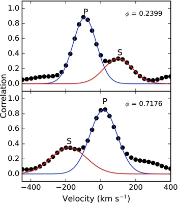
Figure 2. Cross-correlation functions of two spectra obtained in orbital quadratures. The letter ϕ shows corresponding orbital phase.
We give log of observations in Table 1, together with measured radial velocities and their standard errors. Orbital phases in the table are calculated via ephemeris and period given in Borkovits et al. (Reference Borkovits2016), which we also adopt for further analysis. Investigating Table 1, one can easily notice the large standard error values for the measured radial velocities of secondary component. This is primarily caused by the small contribution of the secondary component to the total spectrum of the system, which can be evaluated from the cross correlation peaks of components given in Figure 2. We note that 3 600 s of exposure time corresponds to 0.025 orbital phase step and estimated radial velocity shift during this exposure time is about 8 km s−1at the orbital quadratures for the secondary component, and much smaller for the primary component. These shifts are negligible compared to the standard errors of the measured radial velocities; therefore, we can safely ignore the velocity shift due to the long exposure time.
Preliminary light curve examination of KIC 7385478 indicates no evidence for eccentric orbit; therefore, we calculate spectroscopic orbital elements of the system by assuming circular orbit. In addition, we fixed the orbital period and ephemeris to the values given by Borkovits et al. (Reference Borkovits2016). We use a simple python script written by us, which applies differential corrections by least squares method to all radial velocities, as described in Aitken (Reference Aitken1935). We tabulate calculated spectroscopic orbital elements in Table 2 and plot measured radial velocities together with theoretical spectroscopic orbit and residuals from solution in Figure 3. Residuals, which belongs to the primary component scatters over zero level, while the residuals of the secondary component occupy the sub-zero level and this may be interpreted as if the whole fit could be improved further. However, if one consider the total rms of the fit given in Table 2 (last row) as one σ, then the scatter of residuals is inside ~ 1.5 σ level and indicates that any further improvement to the orbital solution has no statistical significance, but only cause slight changes in stellar parameters, which would still stay inside corresponding standard error.
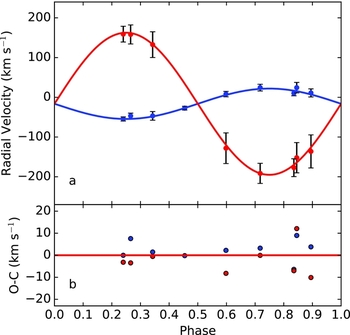
Figure 3. (a) Observed radial velocities of the primary and the secondary (blue and red filled circles, respectively) and their corresponding theoretical representations (blue and red curve). (b) Residuals from theoretical solution.
Table 2. Spectroscopic orbital elements of KIC 7385478. M 1 and M 2 denote the masses of the primary and secondary component, respectively, while M shows the total mass of the system.
3.3. Light curve modelling
In case of KIC 7385478, light curve modelling would not be practical by considering 65 722 long cadence data points; therefore, we first phase the whole data with respect to the orbital period and then calculate binned light curve with a phase step of 0.002 by using freely available fortran code lcbin Footnote 6 written by John Southworth. We use the phase binned light curve for modelling the eclipsing binary. The first step of the light curve modelling is to find geometric and physical parameters of the system, based on phase binned data and the second step is to calculate theoretical light curve with the best geometric and physical parameters and subtract the theoretical model from the whole long cadence data in order to inspect possible out of eclipse variations. We plot the phase binned light curve in Figure 4, panel a.

Figure 4. (a) Phase binned light curve of KIC 7385478 (black filled circles) together with best fit models with and without spot (yellow and red curves, respectively). (b) Close up view of the light curve at light maxima. Panel (c) and (d) show residuals from the solutions without and with spot, respectively.
By the quick inspection of the phase binned light curve, one may see that the system is on a circular orbit and there is a possibility of semi-detached configuration for the system. It may also be noticed that light level around 0.75 phase is slightly higher than the light level around 0.25 phase (see Figure 4, panel b), which means this effect is dominant through 4 yrs of Kepler observations. Difference in the depth of the primary and secondary minima is another important feature of the light curve, which indicates large difference between the temperatures of the components. Shape of the light curve at out of eclipse phases indicates variations beside the geometric eclipse events, such as distortion in geometric shape of the components, reflection, spots, and even oscillations as we will focus on in the next section.
We use 2015 version of the Wilson–Devinney code (Wilson & Devinney Reference Wilson and Devinney1971; Wilson & Van Hamme Reference Wilson and Van Hamme2014) for light curve modelling. Thanks to our spectroscopic observations, we have already determined the two most critical parameters of the light curve modelling process, i.e. effective temperature of the primary component and the mass ratio of the system. We fixed these two parameters during the modelling. Since the effective temperature of the primary component is at critical location where the convective outer envelope is very thin or almost becomes radiative, we carried out solutions by setting gravity darkening (g 1) and albedo (A 1) values to 0.32 and 0.5, respectively (for convective envelopes) and setting both parameters to 1.0 (for radiative envelopes). In both cases, there is almost negligible difference between solutions with radiative envelope and convective envelope assumption, where convective envelope assumption leads to a slightly lower residuals; thus, we continue with 0.32 and 0.5 values for g 1 and A 1, respectively. We adopt g 2 and A 2 values as 0.32 and 0.5 for the secondary component, which are typical for convective envelopes. Both light curve and spectroscopic orbit solution indicate circular orbit for the system; therefore, we assume synchronous rotation for the components, which is proper for circular orbits, and fix rotation parameter (F) of each component to 1.0. Here, F is defined as the ratio of the axial rotation rate to the orbital rate. Linear limb darkening coefficients (x 1, x 2) of the components are adopted from van Hamme (Reference van Hamme1993).
We start analysis with detached configuration, therefore, we consider inclination of the orbit (i), temperature of the secondary component (T 2), dimensionless omega potentials of the primary and the secondary component (Ω1, Ω2), luminosity of the primary component (L 1) as adjustable parameters. In addition, we observe a general phase shift of 0.002 in the phase binned light curve, which possibly arises from a shift in the adopted ephemeris due to the third body (Borkovits et al. Reference Borkovits2016); hence, we also adjust phase shift during analysis. In a few iterations, we observe that the Ω2 value jiggles around the inner critical potential value and secondary component has entirely filled its Roche-lobe in the corresponding Roche geometry. Then we switch to the semi-detached configuration and fixed Ω2. In this case, we consider distorted shape of the secondary component and adopt g 2, A 2, and x 2 as adjustable parameters during iterations. After a few iterations, we achieve statistically the best parameter set, however, we still observe that the residuals from the solution exhibit additional wave-like variation through an orbital cycle.
During the iterations, we noticed that the contribution of the secondary component to the total light is not more than 15%; therefore, we expect negligible contribution from the secondary component to the wave-like variation in residuals. The most possible explanation could be that the Roche-lobe filled secondary star transfers its own mass to the primary component through the inner Lagrange point, L1, of the system. The transferred mass possibly hits directly to the photosphere of the primary component without forming an accretion disk, thus forms a local region warmer than the surrounding photosphere. Therefore, we consider this hot region as a bright spot on the primary component and add a single bright spot into our light curve model. At first step, we adopt spot longitude and radius as adjustable parameters together with eclipsing binary parameters and fixed the spot co-latitude and temperature factor to 45° and 1.03, respectively. After these parameters are adjusted, we fix the spot longitude and radius, and adjust spot co-latitude and temperature factor. Until we achieve the best solution, we adjust different number of spot parameters simultaneously with a different combinations. When we reach the best solution, we adopt all parameters (spot and eclipsing binary) adjustable and run a single iteration in order to obtain statistical uncertainties. We tabulate our results in Table 3. Note that we do not give the internal error of the T 2 since it is unrealistically small (~ 1 K); therefore, we adopt the uncertainty of T 1 estimated in Section 3.1 as the uncertainty of T 2. In Figure 4, we over plot the best fit models of spotless and spotted solutions (panel a and b) and show residuals from both solutions in panel c and d in the same figure.
Table 3. Light curve modelling results of KIC 7385478. ⟨r
1⟩ and ⟨r
2⟩ denote mean fractional radii of the primary and the secondary components, respectively. Spot parameters are given in the order of co-latitude (θ), longitude (φ), radius ( $r_{\text{spot}}$
), and temperature factor (
$r_{\text{spot}}$
), and temperature factor ( $\text{TF}$
). Internal errors of the adjusted parameters are given in parentheses for the last digits. Asterix symbols in the table denote fixed value for the corresponding parameters.
$\text{TF}$
). Internal errors of the adjusted parameters are given in parentheses for the last digits. Asterix symbols in the table denote fixed value for the corresponding parameters.
3.4. Physical properties and evolutionary status
Combining results from spectroscopic orbital solution and light curve modelling, we calculate absolute physical parameters of the system listed in Table 4. Inspecting the parameters, we immediately see that the secondary component has a very large radius compared to its mass which causes lower gravity compared to a typical main sequence star. A typical main sequence star has a radius of ~ 0.41 R⊙(Gray Reference Gray2005). Adopting temperature calibration of Gray (Reference Gray2005), we estimate the spectral type of the secondary as K4 III–IV. All these indicate that the lower mass secondary component has already evolved off the main sequence, which seems contradictory to the stellar evolution theory. However, we know that the secondary component has already filled its Roche-lobe and there must be mass transfer from secondary to the primary via inner Lagrange point, L1. The situation could be explained as the secondary component was actually the more massive component in the system and as it evolved off the main sequence, it filled its Roche-lobe and started a mass transfer to the less massive component (in our case, the primary component). We observe the effect of the mass transfer as hot spot on the primary component. Continuous mass transfer in time finally reversed the mass ratio of the system; therefore, the final configuration became like a more massive main sequence star and a less massive sub-giant star. This is typical scenario adopted for Algols, which are well known to have reverted their mass ratio because of Roche-lobe overflow.
Table 4. Absolute physical properties of KIC 7385478. Error of each parameter is given in parenthesis for the last digits.
In Figure 5, we show the position of the primary component of KIC 7385478 on Hertzsprung–Russel diagram, together with some eclipsing binaries with known γ Doradus type pulsating components, i.e. VZ CVn (Ibanoǧlu et al. Reference Ibanoǧlu, Taş, Sipahi and Evren2007), CoRot 102918586 (Maceroni et al. Reference Maceroni, Montalbán, Gandolfi, Pavlovski and Rainer2013), KIC 11285625 (Debosscher et al. Reference Debosscher2013), KIC 9851142 (Çakırlı Reference Çakırlı2015), KIC 9851944 (Guo et al. Reference Guo, Gies, Matson and Hernández2016), V2653 Oph (Çakırlı & Ibanoglu Reference Çakırlı and Ibanoglu2016), CoRot 100866999 (Chapellier & Mathias Reference Chapellier and Mathias2013). Our target is located in the middle of the γ Doradus instability strip given by Warner et al. (Reference Warner, Kaye and Guzik2003), which takes us to the possibility of γ Doradus type pulsation on the primary component.

Figure 5. Position of the primary component of KIC 7385478 on Hertzsprung–Russel diagram (star symbol in blue). Black dots show confirmed γ Doradus stars from Henry, Fekel, & Henry (Reference Henry, Fekel and Henry2005), filled large black circles denote discovered pulsating components in eclipsing binaries. Red dashed lines indicate theoretical cool and hot boundary of γ Doradus instability strip (Warner, Kaye, & Guzik Reference Warner, Kaye and Guzik2003). Black continuous curves show zero age and terminal age main sequences, taken from Pols et al. (Reference Pols, Schröder, Hurley, Tout and Eggleton1998).
3.5. The out-of-eclipse variations
In order to inspect the out-of-eclipse variations, we first construct a theoretical light curve by using the parameters in Table 3, then subtract it from whole long cadence data and obtain residuals. In this process, we first divide the whole long cadence data into subsets where each subset covers a single orbital cycle. Then, we run differential correction programme of the Wilson–Devinney code by only adjusting ephemeris reference time of the related subset and keeping all remaining parameters fixed. This process eliminates any shift in the ephemeris reference time due to the light time travel effect caused by the third body and gives correct residuals.
In Figure 6, we plot the whole residuals (panel a), and a sample of residuals covering a time span of a month (panel b and c). One may easily notice that removing eclipsing binary model from the data unravels a clear variation with a dominant period of ~ 0.5 d (panel b) with variable amplitude, which suggests the possibility of γ Doradus type pulsation (Kaye et al. Reference Kaye, Handler, Krisciunas, Poretti and Zerbi1999) on the primary component, with a beat period of about 12 d. In addition, we observe occasional increase in amplitude of residuals (panel c), where the most dominant period becomes the orbital period, however, by keeping 0.5 d variation as small humps and pits through an orbital cycle.
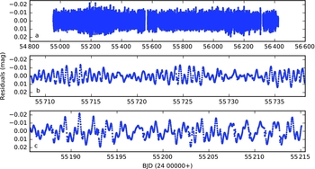
Figure 6. (a) Residuals from whole long cadence data. (b) Portion of residuals around BJD = 2 455 723, where the variation amplitude is smaller. (c) Residuals around BJD = 2 455 200, where the variation amplitude is larger.
We apply multi-frequency analysis to the residual data using pysca software package (Herzberg & Glogowski Reference Herzberg and Glogowski2014) to investigate these variations. In case of continuous and long time series photometry, pysca is very practical to automatically extract significant frequencies above a defined SNR limit. We start with Fourier analysis of the data for the frequency between 0 and 24.498 cycle/d (c/d), where the 24.498 denotes the nyquist frequency. In Figure 7, we show amplitude spectrum of the residuals (panel a). We observe that the dominant frequencies are located in lower frequency region (f < 5 c/d) and consider this region for frequency extraction process. In this process, the most dominant frequency in the amplitude spectrum is determined. Then its amplitude and phase are calculated via $A_{\text{i}} \Sigma \text{sin}[2\pi (f_{\text{i}}t + \phi _{i})]$
, where t is the time of the corresponding measurement, while
$A_{\text{i}} \Sigma \text{sin}[2\pi (f_{\text{i}}t + \phi _{i})]$
, where t is the time of the corresponding measurement, while $A_{\text{i}}$
,
$A_{\text{i}}$
, $f_{\text{i}}$
, and
$f_{\text{i}}$
, and $\phi _{\text{i}}$
show the amplitude, frequency, and phase of the ith frequency, respectively. Next, this frequency is removed from the data and the same process is repeated for the remaining ‘prewhitened’ residuals. We adopt criteria of Breger et al. (Reference Breger1993), which puts a lower SNR limit of 4 for a frequency to be accepted as significant. Uncertainties of the extracted frequencies are estimated as ~ 7 × 10⁻³ d−1, which is determined by using the Rayleigh criterion.
$\phi _{\text{i}}$
show the amplitude, frequency, and phase of the ith frequency, respectively. Next, this frequency is removed from the data and the same process is repeated for the remaining ‘prewhitened’ residuals. We adopt criteria of Breger et al. (Reference Breger1993), which puts a lower SNR limit of 4 for a frequency to be accepted as significant. Uncertainties of the extracted frequencies are estimated as ~ 7 × 10⁻³ d−1, which is determined by using the Rayleigh criterion.

Figure 7. (a) The whole amplitude spectrum of the residuals. (b) Close view of the frequency range where the orbital frequency is located. Panel c and d are similar to the panel b but for pulsation frequencies.
This process leads to 735 frequencies above SNR limit of 4. The most dominant two peaks are located at 2.0252 and 1.9427 c/d, corresponding 0.4938 and 0.5147 d and we define these frequencies as γ Doradus type pulsation frequencies. Third and fourth peaks are 0.6034 and 0.6023 c/d, corresponding 1.6573 and 1.6603 d, and these frequencies indicate the orbital frequency. Beyond the first four frequencies, we do not find any independent frequency but low- and high-order combination of pulsation and orbital frequencies. We list the extracted frequencies in Table A1.
In Figure 7, we also show close view around orbital frequency (panel b) and pulsation frequencies (panel c and d). One may easily notice that peaks at pulsation frequencies are single and sharp peaks, while the peak at the orbital frequency is more shallow in amplitude and broader. This picture leads us to calculate amplitude spectrum of long cadence data for each Kepler data quarter separately and investigate behaviour of the dominant peaks in 4 yrs time range. We plot amplitude spectrum of each quarter separately in Figure 8. Amplitudes of the pulsation frequencies are almost stable in all quarters, while the amplitude of the orbital frequency clearly varies in time, which causes shallow and broader peak(s) at the orbital frequency in the amplitude spectrum of the 4 yr long cadence data.

Figure 8. Amplitude spectrum of each quarter. We mark the location of the orbital frequency and the most dominant two frequencies (i.e. pulsation frequencies) with red vertical dashed lines and label each plot window according to its quarter number. Note that Q0 and Q17 contain less number of data points compared to the other quarters, thus peaks of dominant frequencies are broad in their amplitude spectrum.
4 SUMMARY AND DISCUSSION
Photometric and spectroscopic analysis of KIC 7385478 shows that the system is a low mass ratio (q = 0.21) eclipsing binary formed by an F1V primary, and a K4III–IV secondary components which entirely fills its Roche-lobe. This means the system can be classified as semi-detached. Physical properties of the components suggest that the low mass secondary component has already evolved off the main sequence before the dwarf primary component, which is not expected in the scope of the stellar evolution theory. Continuous mass transfer between the components could explain this situation, which could change the roles (and masses) of the components in long time scales. If the mass transfer does not lead to a disk, a hot spot forms on the photosphere of the mass gaining component, where the streaming matter directly hits to its photosphere. Almost continuous Kepler long cadence photometry through 4 yrs indicates a brightness level difference between orbital quadrature phases (i.e. 0.25 and 0.75 phases), which could be explained by this kind of a hot spot on the primary (mass gaining) component. At that point, the assumption of an impact system (no disc) can be justified by the mass ratio (0.22) and fractional radius of the primary (0.21) according to Lubow–Shu criterium (Lubow & Shu Reference Lubow and Shu1975) for disc formation. Furthermore, we do not observe any emission feature in Hα, indicates the absence of the disk and this is consistent with impact system assumption.
The position of the primary component on HR diagram corresponds to the middle of the region where γ Doradus variables are located and suggests intrinsic light variations related to pulsation. When we subtract the eclipsing binary model from the long cadence data, we see clear signal which has a dominant period of ~ 0.5 d indicating γ Doradus type pulsations and confirms the intrinsic variation suggested by the position on HR diagram. However, we also observe occasional increase in the amplitude of the residuals where the dominant period becomes the orbital period, including ~ 0.5 d variation as a smaller amplitude variation. Multiple frequency analysis of the residuals results in 735 frequencies, where the first two frequencies indicate γ Doradus type pulsations, while the third and the fourth frequencies correspond to the orbital frequency. Most of the remaining 731 frequencies correspond to either the orbital frequency or its harmonics. This indicates an additional light variation with a period almost identical to the orbital one and this variation is usually suppressed by the light variation originating from pulsations.
Figures 7 and 8 clearly show that the amplitude of the orbital frequency varies in time and this causes broad and shallow peak structure at the orbital frequency in amplitude spectrum of 4 yr data, which is another evidence for the additional light variation mentioned above. Possible star spot activity originating from the cool secondary component could easily cause this kind variation, thus leads to many low- and high-order combinations of the pulsation and orbital frequencies in the amplitude spectrum, especially in period analysis of continuous long-term data, which covers ~ 4 yrs in case of KIC 7385478. It is also known that stellar magnetic activity may cause orbital period modulations via mechanism proposed by Applegate (Reference Applegate1992). Another possibility for orbital period modulations is variable mass transfer rate in the donor. Since the typical time scales for Applegate mechanism and variable mass transfer rate are decades or longer, these are not comparable to the modulations observed in residual data of KIC 7385478, therefore are not likely.
Estimated spectral type and luminosity class of the secondary component provide support for the spot activity possibility. According to the eclipsing binary model, 14% contribution of the secondary component to the total light is expected at very broad band Kepler filter, which means we may observe small amplitude light variation due to the possible spot activity of the secondary star. However, when we check the observed spectra of the system, we do not observe any emission feature in Ca ii H & K lines, which are very sensitive to the chromospheric activity in cool stars. Considering the temperatures and radii of the components, one may easily conclude that the contribution of the secondary component to the total light around 3 950 Å is almost completely negligible, hence, considering only the spectroscopic indicators, we may not arrive at the conclusion on the existence of star spot activity in case of KIC 7385478. Therefore, we can still speculate that the secondary component might have star spot activity, which seems the most possible cause of the occasional amplitude increase in the light residuals.
ACKNOWLEDGEMENTS
We thank to TUBITAK for a partial support in using RTT150 (Russian-Turkish 1.5-m telescope in Antalya) with project number 14BRTT150-667. This paper includes data collected by the Kepler mission. Funding for the Kepler mission is provided by the NASA Science Mission Directorate. Some of the data presented in this paper were obtained from the Mikulski Archive for Space Telescopes (MAST). STScI is operated by the Association of Universities for Research in Astronomy, Inc., under NASA contract NAS5-26555. Support for MAST for non-HST data is provided by the NASA Office of Space Science via grant NNX13AC07G and by other grants and contracts.
A Multi-frequency analysis results
Table A1. Extracted frequencies in multi-frequency analysis. N, F, A, P, and SNR means number, frequency (in c/d), amplitude (in mmag), phase, and signal-to-noise ratio, respectively.


