2. Formulation of the problem

2.1. Problem set-up

The initial flow field is a quasi-Gaussian or the Lamb–Oseen vortex (Fabre, Sipp & Jacquin Reference Fabre, Sipp and Jacquin2006; Mao & Hussain Reference Mao and Hussain2017). Non-dimensionalising the lengths by the ring radius $R_0$, the vortex profile is centred at $(x, \eta )=(0, 1)$, and its non-dimensional velocity components in the $(x, \eta, \phi )$ coordinates (see figure 1) are written as

(2.1)\begin{gather} u_{x}=\frac{\varGamma_0}{2{\rm \pi}}\frac{1-\eta}{x^2+(\eta-1)^2} ( 1- {\rm e}^{-(x^2+(\eta-1)^2)/{a^2}} ), \end{gather}

(2.2)\begin{gather}u_{\eta}=\frac{\varGamma_0}{2{\rm \pi}}\frac{x}{x^2+(\eta-1)^2}( 1- {\rm e}^{-(x^2+(\eta-1)^2)/{a^2}}), \end{gather}

(2.3)\begin{gather}u_{\phi}=0, \end{gather}

where $\varGamma _0$ is the initial circulation and $a$ is the initial radius of the vortex core. Here, $a/R_0=0.2$ is applied throughout this work. The initial bubble is spherical, with a size of $R_b/R_0=0.284$ and a distance $0.2R_0$ from the ring centre. We note that the induced velocity has an axial component of $1/{2{\rm \pi} } \approx 0.159$ at the centre of the vortex ring, i.e. $u_x \approx 0.159$ at $(x, \eta )=(0, 0)$. To initialise the vortex ring from being perfectly circular, we perturb the local radius $\eta$ by adding a small parameter $\zeta \ll 1$ multiplied by the sum of a set of $N$ Fourier modes, each with unit amplitude and random phase, as adopted in a previous study (Archer, Thomas & Coleman Reference Archer, Thomas and Coleman2008). After initialisation, the flow is relaxed quickly to the real solution by solving the Navier–Stokes equations. The velocity in the cylindrical coordinate system, written in (2.1) to (2.3), can be easily transformed to the Cartesian coordinate system used in our three-dimensional simulations.

Figure 1. A vortex ring and a gas bubble in the cylindrical coordinate system, where $x, \eta$ and $\phi$ are the axial, radial and azimuthal coordinates respectively, and the origin $O$ is at the centre of the ring. The gas bubble is released initially at the $x$ axis with a short distance $0.2R_0$ from $O$, as illustrated in this figure.

2.2. Numerical method

The flow involving two immiscible phases can be solved using a single-fluid continuum approach. We solve the time-dependent Navier–Stokes equations in incompressible form under a finite-volume framework, considering the translation of a liquid vortex ring and the deformation and translation of a gas bubble induced by the vortex ring. The differential forms of the governing equations are

(2.4)\begin{gather} \boldsymbol{\nabla}\boldsymbol{\cdot}\boldsymbol{u}=0, \end{gather}

(2.5)\begin{gather}\frac{\partial\rho\boldsymbol{u}}{\partial t}+\boldsymbol{\nabla}\boldsymbol{\cdot}(\rho\boldsymbol{uu})={-}\boldsymbol{\nabla} p +\rho\boldsymbol{g}+\boldsymbol{\nabla}\boldsymbol{\cdot}\boldsymbol{\tau} +\boldsymbol{F}_{\sigma}, \end{gather}

where $\boldsymbol {u}$ is the velocity vector, $p$ is pressure, $\boldsymbol {g}$ is the gravitational acceleration pointing in the negative direction of the $x$ axis, $\boldsymbol {\tau }$ represents the deviatoric stress tensor, $\boldsymbol {F}_{\sigma }$ is included to represent the surface tension of the liquid–gas interface and $\rho$ and $\mu$ are the mixture density and dynamic viscosity of the fluid, respectively, defined as

(2.6)\begin{gather} \rho = \varphi \rho_l + (1-\varphi)\rho_g, \end{gather}

(2.7)\begin{gather}\mu = \varphi \mu_l + (1-\varphi)\mu_g. \end{gather}

The subscripts $l$ and $g$ represent respectively the liquid and gas phases. The density ratio $\rho _l /\rho _g$ is set to be 1000, approximating that between water and air. Here $\varphi$ is the volume fraction of liquid that has a value of one in the liquid and zero in the gas. In the volume-of-fluid method, $\varphi$ represents volume fractions of one of the two fluids and varies smoothly between 0 and 1. The interface can be defined as the surface where the value of $\varphi$ is equal to 0.5. The volume fraction $\varphi$ is evolved using the following advection equation:

(2.8)\begin{equation} \frac{\partial\varphi}{\partial t}+\boldsymbol{\nabla}\boldsymbol{\cdot}(\varphi \boldsymbol{u})=0.\end{equation}

An algorithm called isoAdvector (Roenby, Bredmose & Jasak Reference Roenby, Bredmose and Jasak2016) based on the volume-of-fluid method is used to reconstruct geometrically and advect the phase interfaces. This algorithm is satisfactory in terms of volume conservation, boundedness, surface sharpness and efficiency. The surface tension term $\boldsymbol {F}_{\sigma }$ in (2.5), at any point on the interface, assuming the interfacial tension $\sigma$ is constant, can be obtained as

(2.9)\begin{equation} \boldsymbol{F}_{\sigma}={\sigma\kappa}\boldsymbol{\nabla}\varphi, \end{equation}

where $\kappa$ is the curvature of the interface calculated by the continuum surface force method (Brackbill, Kothe & Zemach Reference Brackbill, Kothe and Zemach1992).

To provide satisfactory accuracy in space for the evolution of the vortex ring, as well as that of the gas bubble, several levels of refinements are applied to an initially uniform Cartesian grid. The mesh cells in a box, which encloses the vortex ring and its later developed flow structure, have a length of $0.01R_0$ in all three dimensions. In a smaller box, which encloses the gas bubble, the cell length is $0.005R_0$. Therefore, 80 cells are distributed along the bubble diameter. The whole computational domain has approximately 35 million cells. To ensure spacial accuracy as the flow evolves, we move the computational domain axially with the speed at which the vortex ring translates. The integral form of the governing (conservation) equations defined in a moving volume $V$ bounded by a closed surface $S$ can be found in our previous study (Deng & Caulfield Reference Deng and Caulfield2018). As the volume $V$ is no longer fixed in space, its motion is captured by the motion of its bounding surface $S$ at the boundary velocity $\boldsymbol {u}_s$.

The space discretisations for (2.5) are second-order upwind for the convection terms and central differences for the Laplacian terms. The temporal term is discretised by the implicit Crank–Nicolson method. The pressure–velocity coupling in incompressible flow simulation is obtained using the pressure-implicit with splitting of operator scheme (Ferziger, Perić & Street Reference Ferziger, Perić and Street2002). At the outer boundary of the computational domain (a cube with a side length of $100R$) we set the normal components of the velocity gradients to be zero, and the pressure (excluding the hydrostatic pressure) to be zero. To ensure time-discretisation independence, we choose the size of time step, meeting the requirement $Co=\delta t |\boldsymbol {U}|/\delta x <1$ for all cells, in which $|\boldsymbol {U}|$ is the magnitude of the velocity through a cell and $\delta x$ is the cell width in the direction of the velocity.

2.3. Non-dimensional parameters

Since the vortex ring at $Re_\varGamma =7500$ has been extensively studied by both experimental measurements (Weigand & Gharib Reference Weigand and Gharib1994) and numerical simulations (Bergdorf, Koumoutsakos & Leonard Reference Bergdorf, Koumoutsakos and Leonard2007), we fix this Reynolds number for most simulations. Here, $Re_{\varGamma }$ is defined as

(2.10)\begin{equation} Re_\varGamma=\rho_l\frac{\varGamma_0}{\mu_l}, \end{equation}

where $\mu _l$ is the dynamic viscosity of the liquid. The Weber number, which is a measure of the relative importance of the fluid's inertia compared to its surface tension, is defined as

(2.11)\begin{equation} We=\frac{0.87\rho_l(\varGamma_0/2{\rm \pi} a)^2}{(\sigma /D_b)}, \end{equation}

following a previous study (Oweis et al. Reference Oweis, Van der Hout, Iyer, Tryggvason and Ceccio2005), which may be thought of as the ratio of the pressure difference (${\rm \Delta} P=0.87\rho (\varGamma _0/2{\rm \pi} a)^2$) between the vortex core and the far field to the Laplace pressure ($\sigma /D_b$) for a spherical bubble. In this study, $We$ varies in the range of 130.5–870. We also note that for a freely rising gas bubble in quiescent liquid, it can be characterised by two parameters, the Eötvös number and the Galileo number, defined respectively as

(2.12a,b)\begin{equation} Eo=\frac{\rho_{l}gD_b^{2}}{\sigma} \quad {\rm{and}}\quad Ga=\frac{\rho_{l}^{2}gD_b^{3}}{\mu_{l}^{2}},\end{equation}

where $g$ is the magnitude of gravitational acceleration and $D_b$ is the diameter for an equivalent spherical bubble (here $D_b=2R_b$). According to the currently chosen parameters, $Ga$ is fixed at $43.2$, and $Eo$ varies from $0.00048$ to $0.016$, corresponding to a perfectly spherical bubble when it is driven only by buoyancy force (Tripathi, Sahu & Govindarajan Reference Tripathi, Sahu and Govindarajan2015). A direct comparison between the $We$ and $Eo$ ranges indicates that the flow induced by the vortex ring plays a profoundly more significant role than the buoyancy force.

3. Transition of the vortex ring at $Re_\varGamma =7500$

For a translating vortex ring, its main instability is referred to as the Tsai–Widnall instability, or azimuthal instability, which leads to an extensive bending of the initially circular vortex lines. Following a previous study (Archer et al. Reference Archer, Thomas and Coleman2008), in three-dimensional isosurface plots, we distinguish between the region of intense vorticity at the core centre, which is called the ‘inner core’, and the surrounding outer-core region of lower vorticity, which we call ‘halo’ vorticity, as shown in figure 2. It is seen that after the formation of a number of standing waves around the core azimuth, due to a narrow band of independently growing linear instability modes, the flow enters into a nonlinear transition phase. At the early stage, the constructive interference between different modes causes a noticeable ‘lop-sidedness’ to the wave growth and associated core displacement. As shown in figure 2(b), the inner-core displacement becomes appreciable and the halo vorticity rolls up into an interwoven mesh of secondary structure, which consists of a series of loops encompassing the inner core. We note that neighbouring loops are of alternating signed vorticity, and two loops wrap around each azimuthal wave (see figure 2a), consistent with previous experimental observations (Dazin, Dupont & Stanislas Reference Dazin, Dupont and Stanislas2006b) and simulations (Bergdorf et al. Reference Bergdorf, Koumoutsakos and Leonard2007; Archer et al. Reference Archer, Thomas and Coleman2008).

Figure 2. Three-dimensional isosurface visualisations of the secondary structures at $t^*=130$ (a,b) and $t^*=160$ (c,d), where $t^*=t\varGamma _0/R_0^{2}$. In (a,c), the dark-grey surfaces correspond to the inner-core regions $|\omega |R_0^2/\varGamma _0=2.8$; the red and blue surfaces correspond to $\omega _x R_0^2/\varGamma _0=0.85$ and $\omega _x R_0^2/\varGamma _0=-0.85$ respectively, visualising the secondary structure. In (b,c), the light-grey surfaces correspond to $QR_0^4/\varGamma _0^2=0.2$.

At later times, the stationary coherent vortical structure found during the laminar and transitional phases is superseded by the swirling of vorticity filaments, as seen in figure 2(c,d). The core region is no longer stationary, but bends and twists with time, with vorticity filaments similar to the secondary structure generated continually. The vorticity filaments circulate around the core and gradually pass out of the vortex bubble and into the wake as a stream of vorticity filaments and hairpin vortices.

Transforming the simulated results back to the cylindrical coordinate system, we can investigate the global behaviour of flow evolution more conveniently. The circulation can be obtained by

(3.1)\begin{equation} \varGamma = \int_{{-}L}^{{+}L} \int_{0}^{\infty} \langle \omega_\phi \rangle \, {\rm d}\eta \,{\rm d}\kern0.06em x, \end{equation}

where $\langle \omega _\phi \rangle$ represents the mean azimuthal vorticity. The centre of the vortex ring in the ($x,\eta$) space is evaluated by

(3.2a,b)\begin{equation} x_o = \int_{{-}L}^{{+}L} \int_{0}^{\infty} x \langle \omega_\phi \rangle \, {\rm d}\eta \, {\rm d}\kern0.06em x,\quad \eta_o = \int_{{-}L}^{{+}L} \int_{0}^{\infty} \eta \langle \omega_\phi \rangle \, {\rm d}\eta \, {\rm d}\kern0.06em x. \end{equation}

To quantitatively study the characteristics of azimuthal instabilities, we perform the Fourier analysis of the axial vorticity $\omega _x(x,\eta,\phi )$. For each $\eta \unicode{x2013}\phi$ plane, the azimuthal component decomposition of $\omega _x$ is written as

(3.3)\begin{equation} \omega_k (x,\eta,\phi,t)=C_k(x,\eta,t) \cos (k\phi)+S_k(x,\eta,t) \sin (k\phi),\end{equation}

where $C_k$ and $S_k$ represent the Fourier coefficients defined by

(3.4)\begin{equation} \{ C_k(x,\eta,t),S_k(x,\eta,t) \} =\frac{1}{\rm \pi} \int_{0}^{2{\rm \pi}}\omega_x (x,\eta,\phi,t) \{ \cos(k\phi), \sin (k\phi) \} \, {\rm d}\phi.\end{equation}

Based on this decomposition, a measure of the amplitude of the azimuthal component of $\omega _x$ for each wave number on the axial plane is given by

(3.5)\begin{equation} A_k(x,t)=\left( \int_{0}^{2{\rm \pi}} \int_{0}^{\infty} {\omega_k^2 (x,\eta,\phi,t)} \eta \, {\rm d}\eta \, {\rm d} \phi \right)^{{1}/{2}}. \end{equation}

To investigate the development of instability, we measure the first 30 modes at three different $x$ slices, as shown in figure 3(a–d). It is clearly shown that the streamwise vorticity, $\omega _x$, appears with the onset of the Widnall instability, which is apparent in the excitation of the linear unstable mode $k=8$ (Bergdorf et al. Reference Bergdorf, Koumoutsakos and Leonard2007). At the early stage, $\omega _x$ is relatively weak from the pattern of $\omega _x$, as shown at $t^*=120$. With the rapid evolution of the secondary instability, energy is transferred to the second and third harmonics $k=16$ and $k=24$, as shown in figure 3(c) for $t^*=140$. With the vortices breaking into small-scale ones, the dominant mode and its harmonics decay rapidly and all the modes exhibit the same order of magnitude in figure 3(d), indicating the flow transition to a turbulent state. These observations agree well with the previous findings in both experiments (Dazin, Dupont & Stanislas Reference Dazin, Dupont and Stanislas2006a; Dazin et al. Reference Dazin, Dupont and Stanislas2006b) and numerical simulations (Bergdorf et al. Reference Bergdorf, Koumoutsakos and Leonard2007). To further confirm the turbulent state as the nonlinear instability fully develops, we present the energy $E_k$ for different azimuthal modes in figure 4(a), which can be calculated by

(3.6)\begin{equation} E_k(x,t)=\int_{0}^{2{\rm \pi}} \int_{0}^{\infty} \frac{1}{2}|{\boldsymbol{u}_k^{\prime}(x,\eta,\phi,t)}|^2 \eta \, {\rm d}\eta \, {\rm d} \phi,\end{equation}

where $\boldsymbol {u}_k^{\prime }$ is the azimuthal component decomposition of the fluctuation velocity, i.e. the flow velocity subtracting the average translating speed of the vortex ring. It is identified that the law of energy decay follows a characteristic $k^{-5/3}$ law, indicating that the vortex ring has broken into a turbulent state. Alternatively, we create a structured $256\times 256 \times 256$ isotropic mesh, enclosing the vortex ring, and map the flow velocities onto this mesh. Integrating over all wavenumbers $\boldsymbol {k}_2$ of magnitude $|\boldsymbol {k}_2|=k$ for the trace of a velocity-spectrum tensor, we obtain the energy-spectrum function $E_{k2}$, as shown in figure 4(b) (Pope Reference Pope2000). Here, we use $k_2$ to distinguish from the azimuthal mode number $k$. The inertial subrange characterised by the well-known Kolmogorov $k^{-5/3}$ law is seen more clearly for the higher Reynolds number $Re_{\tau }=15\ 000$, which spans down to a length scale around $0.11R_0$. We should point out that at $Re_{\tau }=15\ 000$ the vortex ring is still in the laminar-transitional regime, without being fully turbulent yet, as noted previously (Foronda-Trillo et al. Reference Foronda-Trillo, Rodríguez-Rodríguez, Gutiérrez-Montes and Martínez-Bazán2021).

Figure 3. (a–d) Development of the first 30 harmonics. The three lines with different colours in the spectra represent different measuring planes $x= x_0-0.5a$, $x_0$ and $x_0+0.5a$ (referring to (3.2a,b)). (e–h) The corresponding $\omega _x$ structures, where the initial vortex ring is marked by a circle.

Figure 4. (a) Development of azimuthal modal energies at three sequential times: $t^*=140$, $t^*=160$ and $t^*=200$, for $Re_{\tau }=7500$. The energy decay for $t^*=200$ follows a characteristic $k^{-5/3}$ law, which is denoted by a dash-dotted line. (b) The traditional Kolmogorov energy spectra for $Re_{\tau }=7500$ and $Re_{\tau }=15\ 000$.

4. Interaction of a vortex ring with a bubble

We now investigate how a bubble affects the evolution of a translating vortex ring and, vice versa, the bubble deformation caused by the strain of the vortical flow. The bubble is released from the position shown in figure 1 at time $t^*=10$, when the vortex ring has relaxed to a divergence-free flow. We present in figure 5 the normalised horizontal position of the vortex ring as it interacts with the bubble for different $We$ cases. The motion of the same ring in the absence of the bubble has also been included as the baseline case. The translation speed at any given instant can be easily obtained as the slope of the position–time data shown. For the vortex ring alone, we know that the formula of translation or convective speed was found as

(4.1)\begin{equation} U_c = \frac{\varGamma_0}{4{\rm \pi} R_0} \left[ \ln \frac{8R_0}{a} + C \right],\end{equation}

where $C$ is a function of the shape of the vorticity distribution and $a$ is a measure of the core radius. For a uniform distribution $C=-1/4$, and for a Gaussian core vorticity distribution $C\simeq -0.558$ (Saffman Reference Saffman1970). For a translating vortex ring, the core spreads over time to be of order $a \sim a_0 + (\nu t)^{1/2} \sim a_0 + (\nu \varGamma )^{1/2}R_0$, where $a_0$ is the initial value of the core radius, indicating that the decay of the translation speed is dominated by viscous diffusion. Fukumoto & Moffatt (Reference Fukumoto and Moffatt2008) estimated the translation speed of a vortex ring in a viscous fluid medium as

(4.2)\begin{equation} U_c = \frac{\varGamma_0}{4{\rm \pi} R_0} \left[ \ln \left( \frac{4R_0}{\sqrt{\nu t}} \right) -0.558 - 3.6716 \frac{\nu t}{R_0^2} \right].\end{equation}

In figure 5, we see that the distance travelled by the vortex ring interacting with a bubble is less than that by the non-interacting vortex ring for all Weber numbers. It is interesting to find that the difference between the ring–bubble interacting case and the baseline ring increases as $We$ is decreased in the low-$We$ cases, i.e. $We=130, 174$ and $217$, implying an increased contribution from the surface tension forces. For example, at $We=130$, there is a significant decline in the translation speed of the ring at early times when it starts to interact with the bubble (see the inset of figure 5), which is more pronounced at later times (see the main plot of figure 5). In contrast, we cannot find a notable monotonic behaviour in the high-$We$ range. This difference between low- and high-$We$ ranges implies a different ring–bubble interacting mechanism, which we discuss in more detail by examining their flow structures.

Figure 5. The horizontal position ($x/R_0$) of the vortex ring as a function of time. The results with different Weber numbers are divided into two groups: data for the low $We$ values are shown with solid lines of different colours and those for the high $We$ values are shown with symbols. The black solid line represents the motion of the same ring without bubbles. In the inset, the data in a smaller time range are shown.

We also plot the histories of the vortex translational velocity in figure 6, in which the decaying speed provided by the empirical formula (4.2) is also presented for reference. In figure 6(a), in the low-$We$ range, we observe that the translational speed of the vortex ring for $We=130$ decays more rapidly, and eventually to a much lower level than the other cases. A comparison between figures 6(a) and 6(b) shows that the low-$We$ range exhibits stronger fluctuations of the translational speed at the early stage, due to the oscillating motion (accelerating and decelerating process) of the bubble along the vortex ring axis before being trapped into the vortex core.

Figure 6. Histories of vortex translational speed for (a) the low-$We$ range and (b) the high-$We$ range. In (a), the black line is the Saffman formula (4.2), which has been shifted to match the numerical results. In the inset of (a), the stepwise decay of the translational velocity is observed for the case without bubbles.

To quantify the strength of secondary flow structure due to the azimuthal symmetry breaking as well as the flow transition to turbulence, we measure the total enstrophy according to the streamwise vorticity, expressed as

(4.3)\begin{equation} \varOmega_x=\frac{1}{2}\int \omega_x^2 \, {\rm d} V. \end{equation}

We show the evolution of $\varOmega _x$ in figure 7. It is seen that the rapid growth of enstrophy is earlier for the ring–bubble interacting cases than that in the absence of a bubble, indicating the earlier appearance of secondary flow structure. In the low-$We$ range, the lowest Weber number, i.e. $We=130$, presents the largest growth rate of enstrophy and reaches the peak earlier than the rest, as shown in figure 7(a). In contrast, we cannot find a strong correlation between Weber number and the evolution of enstrophy in the high-$We$ range, shown in figure 7(b). However, it is interesting to notice that there is a bump around $t^*\simeq 20$ as marked by the dashed circle in figure 7(b), which is due to the separation of the boundary layer around the bubble when it is accelerated or decelerated by the vortex, as addressed in a previous study (Foronda-Trillo et al. Reference Foronda-Trillo, Rodríguez-Rodríguez, Gutiérrez-Montes and Martínez-Bazán2021). The previous study has also addressed that this detached vorticity is responsible for triggering the vortex instability. Clearly, the larger the Weber number, the more intense is this secondary vortex, as the bubble deforms more intensely.

Figure 7. Evolution of enstrophy for the secondary vorticity filaments wrapping around the primary vortex ring in the flow field for (a) the low-$We$ range and (b) the high-$We$ range. The case without a bubble is also included in both panels.

As implied in figure 7, the interaction between the vortex ring and bubble is complicated and correlated to the surface tension forces of the bubble or equivalently the Weber number ($We$). To distinguish between the low- and high-$We$ ranges, we select two representative cases from each, and present their evolution of flow structure and bubble deformation, as shown in figures 8 and 10 for $We=130$ and $We=348$ respectively. In figure 8, at the early stage, we see that the bubble translates with the vortex ring, while staying at the centre of the ring, when the whole flow structure is still symmetric. As seen at $t^*=15$, a small secondary vortex ring is induced by the bubble, which propagates backwards through the primary vortex ring (see $t^*=25$), accompanied by the generation of another secondary ring. The first secondary ring translates further downstream, and eventually disappears in the wake (see $t^*=45$). The repeatedly generated secondary rings perturb the primary one, leading to its azimuthal symmetry breaking, as shown at $t^*=45$ and $t^*=55$. The primary vortex ring then exhibits the same unstable wavenumber, resembling that shown in figure 2, i.e. $k=8$, for the vortex ring in the absence of bubbles. Then, the bubble moves towards the ring core and is captured by it, due to the low pressure within the core (see $t^*=65$). During this process of bubble entertainment, we also notice an overshoot of the bubble, as seen at $t^*=75$. After that, as the bubble re-approaches the ring core, the bubble breaks into two, as seen at $t^*=85$. Here, we note that $We=130$ corresponds to $We_\tau =3$, defined as $We_{\tau }=\rho (\varGamma _0/2 {\rm \pi}R_0)^2 / (\sigma / R_b )$. In a previous study (Foronda-Trillo et al. Reference Foronda-Trillo, Rodríguez-Rodríguez, Gutiérrez-Montes and Martínez-Bazán2021), with a three-dimensional simulation, similar binary breakup of the bubble was also reported at $We_\tau =0.75$ with $R_b/R_0=1/3$, while at a different Reynolds number $Re_\tau =15\ 000$ and the bubble moves in the opposite direction of a translating vortex ring. It is easy to identify that the number of small bubbles is $n=12$ after breakup.

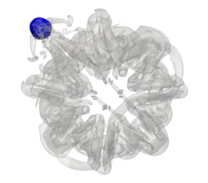
Figure 8. Time sequence of (a) top view and (b) side view images, presenting the interaction of a bubble with a vortex ring at $We=130$. The light-grey surfaces correspond to $QR_0^4/\varGamma _0^2=0.2$. The blue surfaces correspond to the volume fraction of liquid $\varphi =0.5$, representing the translation and breakup of the bubble. Note that the vortex ring translates towards the outside direction of the paper in (a), while from the left to right in (b).

Shown in figure 9 are the magnitudes of the first 30 modes at different time instants for $We=130$, corresponding to figure 8. They resemble the development of the first 30 harmonics without bubbles (see figure 3), while with an earlier transition to turbulent states. The overshoot of the bubble induced by its inertial migration is clearly seen in figure 9(g), resulting in symmetric distributions of the streamwise vorticity regarding the shooting direction.

Figure 9. (a–d) Development of the first 30 harmonics for $We=130$. The spectra are measured on the plane $x=x_0$ (referring to (3.2a,b)). (e–h) The corresponding $\omega _x$ structures, where the initial vortex ring is marked by a circle.

In figure 10, we present the evolution of interacting vortex ring and bubble for $We=348$. The corresponding development of the first 30 harmonics for this case is shown in figure 11. Instead of deviating from the ring centre, as shown in figure 8 for the low-$We$ range, the high-$We$ cases exhibit a significantly different behaviour. Attracted by the low pressure in the ring core, the bubble is stretched radially to a very thin ring, as shown at $t^*=15$. This bubble ring continues to expand in the radial direction, until the surface tension forces cannot keep the integrity of the bubble ring. It breaks into multiple fragments, or small bubbles, as shown at $t^*=20$, where a further expansion of the fragmented bubble ring is seen, as the small bubble reaches the outermost region of the vortex ring. This is followed by a contraction of the bubbles towards the ring centre. After that, the bubbles sit in the centre of the vortex ring core (see from $t^*=25$ to $t^*=65$). As seen at these time instants, the vortex ring encloses a set of smaller bubbles of unequal sizes, which does not further break up, resembling that from a previous experimental visualisation (see figure 1f in Jha & Govardhan (Reference Jha and Govardhan2015)) though with a different set-up. A direct comparison between figures 8 and 10 shows that the secondary vortex filaments become apparent at $t^*=65$ for $We=130$, while at $t^*=85$ for $We=348$, corresponding respectively to their rising stages of the enstrophy histories in figure 7. In figure 10, though much weaker, a secondary vortex ring induced by the spreading bubble can be observed, which stays behind as the small bubbles are entrained into the primary vortex ring, as shown at $t^*=20$.

Figure 10. Time sequence of (a) top view and (b) side view images, presenting the interaction of a bubble with a vortex ring at $We=348$. The light-grey surfaces correspond to $QR_0^4/\varGamma _0^2=0.2$. The blue surfaces correspond to the volume fraction of liquid $\varphi =0.5$, representing the translation and breakup of the bubble. Note that the vortex ring translates towards the outside direction of the paper in (a), while from the left to right in (b).

Figure 11. (a–d) Development of the first 30 harmonics for $We=348$. The spectra are measured on the plane $x=x_0$ (referring to (3.2a,b)). (e–h) The corresponding $\omega _x$ structures, where the initial vortex ring is marked by a circle.

To understand more clearly the stretching, spreading and subsequent breakup process of the bubble, we present in figure 12 the time sequence of the early bubble spreading stage with smaller time intervals. It is interesting to find that the bubble spreads to a flat disk before the thin bubble ring is formed, which gets flatter and flatter until it is torn from the centre, as seen at $t^*=13.5$. The ring bubble breaks into multiple fragments as its radius increases beyond a critical value (between $t^*=16.5$ and $t^*=18$). Here, the critical radius for the bubble ring is identified as $r_c=0.76 R_0$. We also note that the small bubbles move along a spiralling path around the vortex core during the capture process, before they reside in the core centre. Another phenomenon worthy of attention is that at around $t^*=22.5$ when pairs of fine streamwise vortical filaments induced by the small bubbles are observed. It could potentially trigger the azimuthal instability mode of the wavenumber $k=12$, depending on the number of small bubbles. However, this mode of perturbation decays quickly after the bubble capture process completes, with only weak vortex legs remaining in the wake, as seen from $t^*=25$ to $t^*=65$ in figure 10. Instead, the mode $k=8$ instability retakes the dominance, and the primary vortex ring undergoes the secondary transition resembling that without bubbles.

Figure 12. (a–j) Time sequence of vortex–bubble interaction in the early stage, with smaller time intervals, at $We=348$. Note that the light-grey surfaces correspond to $QR_0^4/\varGamma _0^2=0.1$, and the blue surfaces correspond to the volume fraction of liquid $\varphi =0.5$. The vortex ring translates towards the outside direction of the paper.

After examining the vortex–bubble interacting process, it is easy to identify the number of smaller bubbles for each Weber number case. As exhibited in figure 12, there is a fixed, distinguishable number of smaller bubbles before the vortex ring transits further to turbulence. Shown in figure 13 is the number of smaller bubbles as a function of $We$. For the three low-$We$ cases, the number is fixed at 2, while it increases with $We$ in the high-$We$ range, reaching 16 at $We=391$. This maximum number of 16 agrees coincidentally with a previous experimental observation (Jha & Govardhan Reference Jha and Govardhan2015). The number of smaller bubbles keeps at 16 as $We$ further increases, up to the highest Weber number $We=870$ investigated in the current study. From the stretching and spreading process of the bubble observed in figure 12, we conjecture that the classical Rayleigh–Plateau instability is a possible mechanism determining the number of smaller bubbles after breakup, which is a simplified model examining a stretched cylindrical bubble. In this model, the wavelength corresponding to the maximum growth rate for the instability is about 4.5 times the diameter of the cylindrical bubble. In the current study, first, we can identify the maximum radius of the bubble ring, and thereby its azimuthal length $L_b$, before its breakup, as demonstrated in figure 12. Then we can calculate the tube diameter $D_t$ based on the gas volume $V_g$, which does not change due to the conservation of the gas volume, and $L_b$. Lastly, we can estimate the number of smaller bubbles by $n=L_b/(4.5*D_t$). To compare with our numerical simulations, we include the estimated bubble numbers in figure 13. Clearly, the visualised numbers of broken-off bubbles obtained in our simulations agree well with that estimated by the Rayleigh–Plateau instability theory. It is therefore easy to understand that the maximum number of smaller bubbles is limited to 16, due to the fact that the maximum radius of the bubble ring is always smaller than that of the primary vortex ring.

Figure 13. Variation of the number of bubbles with $We$ after complete breakup of the bubble. The number of Rayleigh–Plateau instability waves that fit on the cylindrical bubble is also shown.

In addition, we present the development of modal energies for $We=130$ and $We=348$ respectively in figures 14 and 15. It is not surprising that the energy decay follows a characteristic $k^{-5/3}$ law as the flow develops to fully turbulent states. However, comparing with the case without bubbles (see figure 4) and that with only two broken small bubbles (see figure 14), the $We=348$ case with 12 small bubbles distributed azimuthally along the perturbed vortex ring presents distinctly different spectra, as shown in figure 15, where a clear $k^{-1}$ law is identified. We understand that the $-1$ power region of the turbulence spectrum is a constant energy region responsible for energy production. Here, the $-1$ power region implies the continuous energy injection caused by the two-phase interactions at the early stage of turbulence. However, since it overlaps the inertial range as the turbulence fully develops (see the $-5/3$ power at $t^*=160$), this energy-containing region cannot be distinguished at that time. It will be of interest to simulate at higher Reynolds numbers; then it will be possible to observe these two regions simultaneously. We leave it as an open question.

Figure 14. Development of modal energies for $We=130$ at sequential times: $t^*=68, t^*=85$, $t^*=140$ and $t^*=160$. The energy decay for $t^*=160$ follows a characteristic $k^{-5/3}$ law, which is denoted by a dash-dotted line.

Figure 15. Development of modal energies for $We=348$ at sequential times: $t^*=100$, $t^*=105, t^*=120, t^*=140$ and $t^*=160$. The energy decay for the late time follows a characteristic $k^{-5/3}$ law, while for the time instants $t^*=100$ and $t^*=105$ it follows a characteristic $k^{-1}$, denoted by two dash-dotted lines.

6. Concluding remarks

Differentiating from previous experiments (Jha & Govardhan Reference Jha and Govardhan2015), in which a bubble was released from outside the ring, while following closely their way of analysis, we study numerically the interactions between a vortex ring and a gas bubble released at the axis. As addressed in a previous ‘Focus on Fluids’ paper (Martínez-Bazán Reference Martínez-Bazán2015), which made a brief review and discussion of that experimental work, such an elementary system can represent an idealised scenario providing a framework to shed light on understanding more complicated bubble–turbulence coupling. In the current study, we fix the Reynolds number at $Re_{\tau }=7500$ and consider various Weber numbers in the range of $We=130\unicode{x2013}870$.

First, we investigate the role that bubbles play in the vortex ring dynamics. Clearly shown is that the translating speed of the vortex ring is substantially lower than that of the base of the vortex ring without a bubble. By looking at the enstrophy or volume integral of the square of the streamwise vorticity, we find that the rapid growth of enstrophy is earlier for the ring–bubble interaction cases than that without bubbles, indicating the earlier breaking of azimuthal symmetry, or flow transition. This reduction of ring translating speed, or the earlier flow transition, can be explained with two different mechanisms, depending on the Weber number. For the low-$We$ cases, consistent with that revealed in a previous study (Jha & Govardhan Reference Jha and Govardhan2015), the reduction of convection speed of the ring is due to the capture of bubbles into the ring core, leading to significant changes in the vorticity distribution within the core. However, in the high-$We$ cases, the enstrophy rises before the bubbles are captured into the ring core. Instead, the repeatedly generated secondary vortex rings perturb the primary one, which bring about an earlier flow transition.

On the other hand, we examine the evolution of gas bubbles affected by the strain of the vortical flow. For relatively low Weber numbers, we observe binary breakup of the bubble after it is captured by the primary vortex ring. In contrast, for high Weber numbers, it is interesting to find that the bubble experiences sequentially stretching, spreading and breakup stages. Shortly after release, the bubble spreads to a flat disk, which gets flatter and flatter, until it is torn from the centre, forming a bubble ring. This bubble ring continues to expand in the radial direction, until reaching a critical radius, when the surface tension cannot keep the integrity of the bubble ring. After that, it breaks into multiple fragments, or smaller bubbles. The number of these smaller bubbles is distinguishable. For the three low-$We$ cases, the number is fixed at 2, while it increases from 4 to 16 with $We$ in the high-$We$ range. Furthermore, we find that the numbers of smaller bubbles predicated by the classical Rayleigh–Plateau instability of a stretched cylindrical bubble agree well with our numerical simulations in the high-$We$ range. Consistent with previous experiments (Jha & Govardhan Reference Jha and Govardhan2015), this number reaches 16 as $We$ is sufficiently large.

Additionally, we also investigate the effects of Reynolds number. A direct comparison between two Reynolds numbers reveals that the finer eddies in a vortical field with a higher Reynolds number tend to tear the bubble into more fragments.

A future extension of the present work can be devoted to the cases with even lower Weber numbers, when the breakup of the bubble will not be observed. The critical Weber number for bubble breakup can be identified. Moreover, it would be interesting to examine the effects of gravity, as well as that of the initial bubble position, as a direct comparison with previous experiments. In that scenario, the initial accelerating process of the bubble driven by the buoyancy force will play an important role in the bubble–ring interactions.