


1. Introduction
Gravity currents in porous media have been studied in a wide array of contexts including the geological storage of carbon dioxide (Bickle et al. Reference Bickle, Chadwick, Huppert, Hallworth and Lyle2007; Boait et al. Reference Boait, White, Bickle, Chadwick, Neufeld and Huppert2012), geothermal power generation (Woods Reference Woods1999), contaminant migration (Simmons, Fenstemaker & Sharp Reference Simmons, Fenstemaker and Sharp2001) and coastal aquifer dynamics (Fleury, Bakalowicz & de Marsily Reference Fleury, Bakalowicz and de Marsily2007). When a denser (lighter) fluid displaces a lighter (denser) fluid saturating a porous medium, the density difference causes the displacing fluid to preferentially tilt and flow along the bottom (top) boundary. Huppert & Woods (Reference Huppert and Woods1995) studied this problem assuming the fluids had constant viscosity, the flow was purely horizontal (vertical-flow equilibrium) and there was no mixing between the fluids (sharp-interface limit). They found that the interface between the two fluids tilted, leading to self-similar spreading of the fluids. More recently, the effects of diffusion and vertical flow were considered by Szulczewski & Juanes (Reference Szulczewski and Juanes2013). When the two fluids were fully miscible and vertical flow was accounted for, they found that a series of different regimes arose depending on the dominant physical balances. At intermediate times they found that diffusion and vertical flow could be neglected and the flow reproduced the dynamics outlined by Huppert & Woods (Reference Huppert and Woods1995); however, at early and late times, diffusion played a dominant role in setting the spreading rate.
In addition to having different densities, the two fluids may also have different viscosities, a complication neglected by Huppert & Woods (Reference Huppert and Woods1995) and Szulczewski & Juanes (Reference Szulczewski and Juanes2013). Hesse, Tchelepi & Cantwell (Reference Hesse, Tchelepi, Cantwell and Orr2007), Pegler, Huppert & Neufeld (Reference Pegler, Huppert and Neufeld2014) and Zheng et al. (Reference Zheng, Guo, Christov, Celia and Stone2015) extended the work of Huppert & Woods (Reference Huppert and Woods1995) to study the effect of differing viscosities and densities on the evolution of the displacement front in the limit of sharp interfaces and vertical-flow equilibrium. They found that when the height of the current was comparable to the height of the medium, the viscosity ratio played a dominant role in setting the spreading rate of the gravity current, leading to significantly enhanced spreading if the injected fluid was less viscous than the ambient fluid, or reduced spreading if the injected fluid was more viscous than the ambient fluid. However, similar to Huppert & Woods (Reference Huppert and Woods1995), these works also omit the effects of diffusion and vertical flow. Furthermore, these studies also assumed that the interface between the two fluids was hydrodynamically stable. However, when a less-viscous fluid displaces a more-viscous fluid, viscous fingering can develop and lead to the interpenetration of the two fluids and a highly non-trivial interface (Homsy Reference Homsy1987). Thus far, the effect of viscous fingering on spreading in depth-integrated gravity current models has not been well understood.
In a similar vein, a number of authors have looked at the effect of gravity on the viscous-fingering instability: Rogerson & Meiburg (Reference Rogerson and Meiburg1993b) studied the onset of the viscous-fingering instability with a gravitationally driven shear parallel to the interface using linear stability analysis; Rogerson & Meiburg (Reference Rogerson and Meiburg1993a), Tchelepi et al. (Reference Tchelepi, Orr, Rakotomalala, Salin and Woumeni2004), Tchelepi & Orr (Reference Tchelepi and Orr1994), Ruith & Meiburg (Reference Ruith and Meiburg2000), Camhi, Meiburg & Ruith (Reference Camhi, Meiburg and Ruith2000) and Riaz & Meiburg (Reference Riaz and Meiburg2003) investigated the nonlinear evolution of the fingering instability using numerical simulations; and Tchelepi & Orr (Reference Tchelepi and Orr1994), Berg et al. (Reference Berg, Oedai, Landman, Brussee, Boele, Valdez and van Gelder2010) and Suekane, Koe & Barbancho (Reference Suekane, Koe and Barbancho2019) examined the nonlinear evolution of the fingering instability using laboratory experiments. While these studies highlight some of the interesting qualitative behaviour that can be observed, they do not provide a full overview of the different dynamical regimes, nor do they provide quantitative predictions for the evolution of the concentration field. Furthermore, in all of the work discussed above, the long-time asymptotic behaviour, where diffusion and mixing are important, is neglected.
The overarching aim of this work is to bridge the gap between these two different bodies of work in order to develop a quantitative understanding of the full life-cycle of miscible viscous fingering with gravitational segregation. This work is laid out as follows. In § 2, we formulate the problem and in § 3 consider the two limiting cases of uniform viscosity and uniform density. In § 4 the effects of both density and viscosity differences are examined and the flow phenomenology and dominant dynamical regimes are identified; in §§ 4.1–4.3, these regimes are examined in more detail and reduced-order models for the evolution of the concentration field are derived. Finally, in § 5, the results are summarized and the implications of the results for carbon capture and geological storage are briefly discussed.
2. Problem formulation
We consider a semi-infinite 2-D porous layer with a uniform permeability  $k$ (figure 1). A fluid with density $\rho _1$ and viscosity $\mu _1$ is injected, with a volume flux $Q$, into the medium, which is saturated with an ambient fluid of density $\rho _2$ and viscosity $\mu _2$. We assume that the fluid flow obeys Darcy's law, that the flow is incompressible, and that the concentration $c$ of the injected fluid evolves through the action of advection and diffusion:
 \begin{gather} \boldsymbol{u} ={-}\frac{k}{\mu(c)}\left(\boldsymbol{\nabla} p + \rho g \hat{\boldsymbol{y}} \right), \end{gather}
 \begin{gather}\boldsymbol{\nabla}\boldsymbol{\cdot} \boldsymbol{u} = 0, \end{gather}
 \begin{gather}\phi\frac{\partial {c}}{\partial {t}} + \boldsymbol{u}\boldsymbol{\cdot}\boldsymbol{\nabla} c= \phi D \nabla^{2} c. \end{gather}
Here  $\boldsymbol {u} = (u,v)$ is the Darcy velocity, $p$ the pressure and $D$ an isotropic and constant diffusion coefficient. Note that the injected concentration, $C_i \neq 1$, and the ambient concentration $C_a \neq 0$, can be accounted for with a simple linear rescaling. Following the convention of previous works (Tan & Homsy Reference Tan and Homsy1988; Camhi et al. Reference Camhi, Meiburg and Ruith2000), we assume the viscosity varies exponentially with the concentration
 \begin{equation} \mu(c) = \mu_2 \textrm{e}^{{-}Rc}, \end{equation}
where  $R=\log (\mu _2/\mu _1)$ is the log-viscosity ratio. We employ the Boussinesq approximation and assume a linear relationship between the concentration and the density $\rho$,
 \begin{equation} \rho = \rho_2 + (\rho_1 - \rho_2)c. \end{equation}
Figure 1. A schematic of the model geometry. The porous medium is infinite in the  $\hat {x}$ direction, and finite, with width $a$, in the $\hat {y}$ direction. The medium is initially saturated with a fluid of density $\rho _2$ and viscosity $\mu _2$ and another fully miscible fluid, with density $\rho _1$ and viscosity $\mu _1$ is injected at the left boundary. We assume that the injected fluid is introduced in a purely horizontal manner and at a constant two-dimensional (2-D) volumetric flow rate $Q$.
$Q$.
2.1. Non-dimensionalization
We change to a reference frame moving with the average injection velocity with transformed coordinate  $\tilde {x} = x-Qt/a$ and velocity $\tilde {u} = u-Q/a$. We also incorporate the hydrostatic contributions of the ambient fluid into the pressure field: $\tilde {p} = p + \rho _2 gy$. Non-dimensionalizing by the width of the medium $a$, velocity $Q/a$, advective time scale $\phi a^{2}/Q$, viscosity $\mu _2$ and pressure $\mu _2Q/k$, equation (2.1)–(2.5) become
 \begin{gather} -(\tilde{u}^{*}+1)\mu^{*}= \frac{\partial {\tilde{p}^{*}}}{\partial {\tilde{x}^{*}}}, \quad -v^{*}\mu^{*} = \left(\frac{\partial {\tilde{p}^{*}}}{\partial {y^{*}}} +Gc\right), \end{gather}
 \begin{gather}\frac{\partial {\tilde{u}^{*}}}{\partial {\tilde{x}^{*}}} + \frac{\partial {v^{*}}}{\partial {y^{*}}} = 0, \end{gather}
 \begin{gather}\frac{\partial {c}}{\partial {t^{*}}} + \tilde{u}^{*}\frac{\partial {c}}{\partial {\tilde{x}^{*}}} + v\frac{\partial {c}}{\partial {y^{*}}}= \frac{1}{\textit{Pe}}\left(\frac{\partial^{2} c}{\partial \tilde{x}^{*2}}+\frac{\partial^{2}c}{\partial y^{*2}} \right), \end{gather}
 \begin{gather}\mu^{*} = \textrm{e}^{{-}Rc}, \end{gather}
where  $(^{*})$ denotes a dimensionless quantity. For notational convenience we drop the tildes and asterisks in all subsequent expressions.
There are three important non-dimensional parameters in this problem:
 \begin{equation} R = \log(\mu_2/\mu_1), \quad \textit{Pe} = \frac{Q}{D}, \quad G = \frac{g\left(\rho_1-\rho_2\right)ka}{Q\mu_2}. \end{equation}
The log-viscosity ratio  $R$, measures the strength of the viscosity variations. We will only consider the case $R>0$, that is, when the injected fluid is less viscous than the ambient fluid. The Péclet number, $\textit {Pe}$, measures the relative strength of advection to diffusion. In this work, we will focus predominantly on the geologically relevant limit, $\textit {Pe} \gg 1$. Note that the Péclet number defined here is a macroscopic quantity that depends on the overall size of the porous medium. It is much larger than the pore-scale Péclet number $\textit {Pe}_p=Qb/aD$ which is calculated based on the intrinsic pore scale, $b$, of the porous medium.
Finally, the gravity number,  $G$, measures the ratio of pressure gradients due to density differences and those due to injection. Alternatively, it can be interpreted as a ratio of the vertical rise/fall velocity due to gravity and the horizontal injection velocity. We only consider $G>0$, since $G<0$ is equivalent to $G>0$ with a vertical reflection of the coordinate system $y \rightarrow -y$. Note that the strength of the gravitational force is sometimes defined in terms of a Rayleigh number, $Ra = g(\rho _2-\rho _1)ka/D\mu _2=G\, \textit {Pe}$.
2.2. Boundary conditions
The fluid is injected with a constant horizontal flux, and so in the moving frame
 \begin{gather} \frac{\partial {c}}{\partial {x}} \rightarrow 0 \quad \textrm{as}\ x\rightarrow \pm \infty, \end{gather}
 \begin{gather}\int_{0}^{1} u \,{\textrm{d} y} \rightarrow 0 \quad \textrm{as} \ x \rightarrow \pm\infty, \end{gather}
 \begin{gather}v \rightarrow 0 \quad \textrm{as} \ x\rightarrow \pm \infty. \end{gather}
The last constraint is equivalent to a hydrostatic far-field pressure. There is no flux of concentration through the impermeable upper and lower boundaries of the channel, and so
 \begin{gather} \frac{\partial {c}}{\partial {y}} = 0 \quad \textrm{for}\ y=0,1, \end{gather}
 \begin{gather}v(x,0,t) = v(x,1,t) =0. \end{gather}
No-flux boundaries are critical to allow for the formation of currents that propagate along the boundaries (Rogerson & Meiburg Reference Rogerson and Meiburg1993a; Ruith & Meiburg Reference Ruith and Meiburg2000). We initialize the concentration field to have a step jump,
 \begin{equation} c(x,t=0) = c_0(x) = H({-}x), \end{equation}
where  $H(x)$ is the Heaviside function.
At each time step the velocity field is found using a multigrid relaxation method (Adams Reference Adams1999). The concentration field is advanced in time using a third-order Runge–Kutta scheme, the advective term  $\boldsymbol {u}\boldsymbol {\cdot } \boldsymbol {\nabla } c$ is discretized using a third-order upwinding scheme and the diffusive term $\nabla ^{2} c /\textit {Pe}$ is discretized using a sixth-order compact finite difference method.
2.3. Diagnostic quantities
In order to investigate how the large-scale flow evolves, we focus on quantifying and predicting the evolution of transversely averaged concentration  $\bar {c}(x,t)=\int _0^{1} c\,\textrm {d}y$. Correspondingly, the concentration deviations are defined as $c'(x,y,t) =c(x,y,t) - \bar {c}(x,t)$. Integrating (2.8) over the depth of the porous strip and noting that the flow is incompressible and there is no flux through the top and bottom boundaries yields
 \begin{equation} \frac{\partial {\bar{c}}}{\partial {t}} + \frac{\partial {\overline{u c'}}}{\partial {x}} = \frac{1}{\textit{Pe}}\frac{\partial^{2} {\bar{c}}}{\partial {x}^{2}}. \end{equation}
Subtracting (2.17) from (2.8) gives the evolution equation for the deviations
 \begin{equation} \frac{\partial {c'}}{\partial {t}}+\frac{\partial {\left(u c'\right)}}{\partial {x}}+\frac{\partial {\left(u \bar{c}\right)}}{\partial {x}} -\frac{\partial {\left(\overline{u c'}\right)}}{\partial {x}} + \frac{\partial {\left(vc\right)}}{\partial {y}} = \frac{1}{\textit{Pe}}\left(\frac{\partial^{2} {c'}}{\partial {y}^{2}}+\frac{\partial^{2} {c'}}{\partial {x}^{2}}\right). \end{equation}
 We also examine two macroscopic quantities in time: the spreading length  $h(t)$ (also referred to as the ‘mixing’ length) and the Nusselt number $\textit {Nu}$. We define the spreading length, which measures the length over which the two fluids have spread, as the second spatial moment of the concentration about the initial condition $c_0(x)$ as defined in (2.16),
 \begin{equation} h(t) = \sqrt{\frac{\displaystyle\int_{-\infty}^{\infty}x^{2} (\bar{c}-c_0)^{2} \,{\textrm{d}\kern0.7pt x}}{\displaystyle\int_{-\infty}^{\infty} (\bar{c}-c_0)^{2} \,{\textrm{d}\kern0.7pt x}}} \end{equation}
(cf. Nijjer, Hewitt & Neufeld Reference Nijjer, Hewitt and Neufeld2019). To quantify the rate at which the ambient and injected fluids spread, we define the advective mass exchange through the midplane (travelling with the mean injection velocity),
 \begin{equation} \textit{Nu} = \int_0^{1} (uc)|_{x=0}\, {\textrm{d}y}, \end{equation}
which represents the rate at which the concentration is advectively exchanged between the two fluids. When  $\textit {Nu}=0$, there is no advective exchange: the two fluids simply advect to the right at the injection speed and the interface between the fluids only evolves by diffusion. Larger values of $\textit {Nu}$ indicate more advective exchange across the moving interface. Note that the Nusselt number is often used to quantify the total (advective plus diffusive) transport but here we use it to quantify just the advective transport.
Although not used as a diagnostic quantity, it is useful to combine (2.6a,b), (2.7) and (2.9) and write the velocity in terms of a stream function  $(u,v) = (\partial \varPsi /\partial y, -\partial \varPsi /\partial x)$, as follows:
 \begin{equation} \frac{\partial^{2} {\varPsi}}{\partial {x}^{2}}+ \frac{\partial^{2} {\varPsi}}{\partial {y}^{2}}- R\frac{\partial {\varPsi}}{\partial {x}}\frac{\partial {c}}{\partial {x}}- R\frac{\partial {\varPsi}}{\partial {y}}\frac{\partial {c}}{\partial {y}}= R\frac{\partial {c}}{\partial {y}} + G\,\textrm{e}^{Rc}\frac{\partial {c}}{\partial {x}}. \end{equation}
3. Limiting cases
In this section, we consider two limiting cases: the uniform-viscosity case (log-viscosity ratio  $R=0$) where the fluids differ only in density; and the uniform-density case (gravity number $G=0$) where the fluids differ only in viscosity.
3.1. Uniform viscosity,  $R=0$
$R=0$

When  $R=0$ the problem reduces to the uniform-viscosity gravity-current problem. This situation was studied by Szulczewski & Juanes (Reference Szulczewski and Juanes2013) and we give a brief overview of the dynamics here in order to frame our subsequent more general results. Snapshots of the concentration field from a representative simulation are given in figure 2(a–e). In general, the density difference between the two fluids causes the interface to tilt, with the denser injected fluid travelling along the bottom boundary, which aids in spreading the two fluids. To quantify this spreading, we plot the evolution of the spreading length $h$ in figure 2(f) along with the corresponding theoretical predictions. In general, the spreading length grows in time through five different regimes, each with different power-law growth rates.

Figure 2. Evolution of the concentration field for  $R=0$ and $(G,\textit {Pe}) = (3,100)$. (a–e) Plots of the concentration field versus $x/h(t)$ and $y$ at (a) $t=1\times 10^{-4}$, (b) $t=0.036$, (c) $t=0.83$, (d) $t=57$ (e) $t=8000$. (f) Evolution of the spreading length, $h$, as a function of time, $t$. The dots correspond to the snapshots in panels (a–e) and the dashed lines correspond to the theoretical predictions from Szulczewski & Juanes (Reference Szulczewski and Juanes2013).
First, the concentration field is vertically homogeneous, and longitudinal diffusion dominates, leading to  $h \sim (t/\textit {Pe})^{1/2}$ (figure 2a,f). Second, once longitudinal diffusion becomes unimportant relative to advection, occurring at a time $t\sim O(1/G^{2}\textit {Pe})$, the interface slumps due to gravity. Vertical flow in this regime is important since the vertical length scale of the spreading zone is initially larger than the horizontal scale. This leads to so-called S-shaped slumping and linear growth of the spreading length, $h \sim Gt$ (figure 2b,f). Third, once the interface has become long and thin, that is the horizontal extent of the spreading zone becomes much larger than the vertical extent, occurring at a time $t\sim O(1/G)$, vertical flow becomes unimportant so that the flow is predominantly horizontal. The interface continues to slump due to gravity and takes on a characteristic straight-line profile (figure 2c). The spreading length grows sublinearly, $h\sim (Gt)^{1/2}$, since the hydrostatic pressure gradient, which drives the flow, diminishes as the interface slumps (figure 2f). Fourth, once the interface has become even longer and thinner, occurring at a time $O(Pe)$, transverse diffusion becomes important. A balance between horizontal advection and transverse diffusion results in net horizontal transport analogous to Taylor dispersion (Taylor Reference Taylor1953). However, because the horizontal velocity is proportional to the horizontal gradient in the concentration, the transport is subdiffusive, $h\sim (G^{2}\textit {Pe} \,t)^{1/4}$ (figure 2d,f). Fifth, once the shear-enhanced dispersivity becomes small compared with molecular diffusion, occurring at a time $t\sim O(G^{2}\textit {Pe}^{3})$, the interface grows diffusively again, $h\sim (t/\textit {Pe})^{1/2}$ (figure 2e,f). Note that in each case, the transition times are found by determining the time at which the spreading lengths overlap.
3.2. Uniform density, $G=0$

When  $G=0$, the problem reduces to the miscible viscous-fingering problem studied by Nijjer et al. (Reference Nijjer, Hewitt and Neufeld2018). To review the results of the earlier work, at early times the interface grows diffusively, $h \sim (t/\textit {Pe})^{1/2}$, while the instability grows exponentially (figure 3a,f). At intermediate times, the instability saturates and fingers elongate and interact nonlinearly leading to coarsening and advective growth of the spreading length, $h\sim Rt$ (figure 3b,f). At late times, a single dominant finger is left in the centre of the domain with counter-propagating fingers along the top and bottom boundaries (figure 3c) that eventually slow, leaving a well-mixed interior with constant $h\rightarrow R\textit {Pe}$ (figure 3d,f). Over very long times, in the absence of any advection, the fluid interface evolves purely through longitudinal diffusion and so the spreading length grows like $h\sim (t/\textit {Pe})^{1/2}$.

Figure 3. Evolution of the concentration field for  $G=0$ and $(R,\textit {Pe}) = (2.5,500)$. (a–e) Plots of the concentration field versus $x/h(t)$ and $y$ at (a) $t=2\times 10^{-2}$, (b) $t=2.6$, (c) $t=15$, (d) $t=170$ (e) $t=525$. (f) Evolution of the spreading length, $h$, as a function of time, $t$. The dots correspond to snapshots in panels (a–e) and the dashed lines correspond to the theoretical predictions from Nijjer, Hewitt & Neufeld (Reference Nijjer, Hewitt and Neufeld2018).
One subtle difference between the problem studied in Nijjer et al. (Reference Nijjer, Hewitt and Neufeld2018) and the one studied here is that no-penetration conditions are imposed here along the top and bottom boundaries instead of periodic boundary conditions. We find that up until the late-time regime, this difference in boundary conditions has little effect on the dynamics. However, at late times as the single-finger exchange-flow decays, a pair of wider counter-propagating fingers manifest themselves along the boundaries (figure 3e,f). This is because, in contrast to the case with periodic boundaries, a half-wavelength mode is now permissible (Abdul Hamid & Muggeridge Reference Abdul Hamid and Muggeridge2020). Since this mode is wider, it decays more slowly and is still unstable once the central propagating finger decays away. This mode decays four times more slowly and spreads four times farther but also eventually decays away.
The temporal scalings for the early- to intermediate-time transition and intermediate- to late-time transitions are as before, occurring at times  $t\sim O(1/R^{2}\textit {Pe})$ and $t\sim O(\textit {Pe})$, respectively, again calculated by determining the overlap of the spreading lengths. There is an additional time transition to the half-wavelength mode which occurs at a time $t\sim O(\textit {Pe})$ as well, but with a larger prefactor.
3.3. Comparison of the two limiting cases
There are a number of similarities between the two limiting cases discussed. In both cases, the early-time dynamics are dominated by longitudinal diffusion. At intermediate times diffusion becomes unimportant and spreading is dominated by advection. Initially, vertical flow is important but, as the interface is stretched longitudinally, the flow becomes predominantly horizontal. At late times, there is a balance between horizontal advection and transverse diffusion leading to a slowdown in the flow.
Despite these similarities, the manner in which the systems evolve are very different. In the uniform-viscosity case, there are no hydrodynamic instabilities and the dynamics are insensitive to small changes in the initial conditions, while in the uniform-density case, the interface fingers chaotically and the exact dynamics are highly sensitive to the initial conditions. At intermediate times, in the uniform-viscosity case, the spreading length first grows like  $h\sim t$ then like $h\sim t^{1/2}$ while in the uniform-density case the spreading length grows like $h \sim t$. At late times, the spreading length grows like $h\sim t^{1/4}$ in the uniform-viscosity case but tends to a constant in the uniform-density case. In the uniform-viscosity case, the dynamics are decoupled and independent of the injection flux, whereas in the uniform-density case, injection is critical to the formation of fingers. The aim of the remainder of this work is to outline how the aforementioned similarities and differences evolve as both the viscosity and density are varied away from the limiting cases.
4. Overall dynamics
Consider the case where both the density and viscosity vary ( $G\neq 0, R\neq 0$). Depending on the choice of parameters, a range of different behaviours are possible. In figure 4, we show a series of snapshots in time of the concentration field for a large and a small value of $G$, each showing a range of different dynamics. In both cases the interface is stretched longitudinally and eventually becomes transversely well mixed, but the manner in which the flows reach this final state depend on $G$.
$G$.

Figure 4. Colourmaps of the concentration field for  $(R,\textit {Pe}) = (2,500)$ and (a,c,e,g) $G =0.025$, (b,d,f,h) ${G=2}$. The snapshots are taken at times (a,b) $t=0.05$, (c,d) $t=2$, (e,f) $t=30$ and (g,h) $t=500$. Evolution of (i) the spreading length, $h$ and (j) the Nusselt number, $\textit {Nu}$, for the same parameters as in (a–h).
At very early times, in both cases, molecular diffusion dominates the dynamics. The interface then slumps due to gravity, forming a pair of tongues along the top and bottom boundaries, with the effect being more pronounced for larger  $G$ (figure 4a,b). The slumping is asymmetric, due to the viscosity difference, as the forward-propagating tongue propagates much faster than the backward-propagating tongue (figure 4b). At intermediate times, depending on the relative magnitudes of $G$ and $R$ (and $\textit {Pe}$), the interface may finger (figure 4c) or not finger (figure 4d). When the interface fingers, the fluid spreads more slowly as compared with the non-fingered case (figure 4i,j). Eventually, the fingered interface coarsens until a pair of counter-propagating currents remain which resemble the non-fingered case (figure 4e,f). At late times, in both cases, the interface becomes vertically homogenized and the growth of the spreading length slows and tends to the same value independent of $G$ (figure 4g,h). This is analogous to the shutdown of the viscous fingering instability in the $G=0$ limit. Eventually, horizontal advective transport becomes dominated by Taylor dispersion, analogous to the $R=0$ limit, driven by horizontal gradients in $c$. This too becomes negligible over very long times and molecular diffusion dominates again.
Figure 4(i) shows the evolution of the spreading length for large  $G$, small $G$ and zero $G$. When $G$ is large, the spreading length initially grows like $t$, in a manner analogous to the slumping regime in the uniform-viscosity case. The spreading length then grows with a scaling exponent less than unity before tending to a constant spreading length. When $G$ is small, the dynamics are similar to the uniform-density case $G=0$: the spreading length initially grows diffusively, then advectively, before tending to a constant. However, the nonlinear regime is reached earlier, the prefactor in the fingering regime is larger, and the fingers coarsen directly to the half-wavelength mode. In general, increasing $G$ leads initially to faster growth, but all three examples tend to nearly the same constant spreading length. Over longer times the spreading length grows due to shear-enhanced dispersion and $h \sim t^{1/4}$ (not shown), with a prefactor that increases with $G$ and over even longer times the spreading length grows due to longitudinal diffusion and $h\sim t^{1/2}$, independent of $G$.
$G$.
Figure 4(j) shows the evolution of the advective flux through the midplane,  $\textit {Nu}$. When $G$ is large, the advective flux starts at a maximum and initially decays slowly. After approximately $t=30$, the decay rate increases, characteristic of exponential decay of the flux, before tending to a constant. When $G$ is small, the advective flux initially exhibits power-law growth, then exponential growth, before saturating and fluctuating about a constant value. Eventually the flux coincides with the large $G$ case and decays in the same manner, before tending to a smaller constant. The constant flux corresponds to the shear-enhanced dispersive flux driven by density differences between the two fluids. Over very long times (not shown), the advective flux decays to zero as the interface becomes more stretched. For comparison we show the uniform-density case $G=0$, which grows exponentially, fluctuates about a constant and exponentially decays, before growing again as the single finger state becomes unstable as discussed in § 3.2.
In the following sections we discuss the different regimes that are possible in more detail.
4.1. Early-time slumping regime
Initially, the streamwise concentration gradient between the fluids is large and the concentration is transversely homogeneous. In this case, diffusion across the interface dominates and the concentration evolves diffusively:
 \begin{equation} c = \bar{c} = \frac{1}{2} + \frac{1}{2} \mathrm{erf}\left(-\frac{x}{\sqrt{4t/Pe}}\right). \end{equation}
Once advection begins to outpace diffusion, the interface slumps along the boundaries. This leads to localized regions of fast flow but little motion away from the boundaries. When  $G$ is small, small buoyancy-driven fingers, comparable to the fingering instability, grow along the top and bottom boundaries while fingers along the rest of the interface grow more slowly (figure 5a). This preference for fingering along the boundaries occurs because the difference in density leads to slumping which preferentially perturbs the instability along the boundaries. In this case the density difference perturbs the interface but the growth of the fingers is still dominated by viscous effects. We therefore expect that the spreading length grows in a manner analogous to the viscous fingering instability, and so $h \sim Rt$ and a transition time from the diffusive regime at $t\sim (R^{2}\textit {Pe})^{-1}$ (cf. Nijjer et al. Reference Nijjer, Hewitt and Neufeld2018). This rescaling does a reasonable job of collapsing the data for $G\ll 1$ (figure 6b) and the transition time only weakly depends on $G$. Note that even when $G$ is small, the initial growth of the spreading length is significantly enhanced when compared with the uniform-density case (figure 6b).

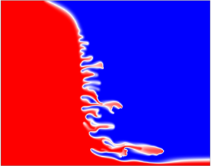
Figure 5. Colourmaps of the concentration field in the slumping regime for  $(R,\textit {Pe}) = (1,4000)$ and $(G,t)=\,$ (a) $(0.02,0.6)$ and (b) $(2,0.07)$.

Figure 6. Plots of  $h(t)$ for $\textit {Pe} = 100$ and different $G$ and $R$ as labelled. The raw data is plotted in (a). In (b) the spreading length is rescaled by the predicted scalings for the small- $G$ slumping limit. The dotted lines denote simulations with $G=0$ and $R=\{0.5,1,2\}$. In (c) the spreading length is rescaled by the predicted scalings for the large- $G$ slumping limit. The dotted lines denote simulations with $R=0$ and $G = \{1,2,4\}$.
When  $G$ is large, the interface slumps on a larger scale which is much faster than the growth of the instability. This form of slumping is analogous to the S-shaped slumping regime in the equal-viscosity case (§ 3.1); however, because the injected fluid is less viscous, the forward-propagating tongue travels faster than the backward-propagating tongue, leading to asymmetric slumping (figure 5b). Based on its similarity with the uniform-viscosity case, we expect that in this regime the spreading length grows like $h \sim Gt$ and a transition from the diffusive regime at $t\sim (G^{2}\textit {Pe})^{-1}$. This rescaling does a reasonable job of collapsing the data for $G> O(1)$ (figure 6c) and the transition time depends only weakly on $R$.
$R$.
4.2. Intermediate-time gravity-current and fingering regimes
At intermediate times, depending on  $t$ and the size of $G$, there are three possible regimes through which the dynamics evolve. These include a viscous-fingering regime where the interface consists of a set of fine fingers and the spreading length grows linearly in time (figure 4c,i), an injection-driven gravity-current regime where the interface is smooth and the spreading length also grows linearly in time but with a larger prefactor (figure 4d,i), and a density-driven gravity-current regime where the interface is also smooth but the spreading length grows like $h\sim t^{1/2}$ (not shown). Depending on the magnitude of $G$ only a subset of these regimes are seen. For small $G$, the interface initially fingers, but over time the fingers coalesce and combine to spread as an injection-driven gravity current. For large $G$, fingering is suppressed and the fluid spreads as a density-driven gravity current before transitioning to an injection-driven one. In the following subsections we aim to delineate these regimes and develop models for how the transversely averaged concentration evolves in each case.
4.2.1. Concentration model
At intermediate times, in all cases, the interface becomes long and thin,  $h\gg 1$ therefore the flow is predominantly horizontal, and longitudinal diffusion is negligible. In this case the flow is in ‘vertical flow equilibrium’ (Yortsos Reference Yortsos1995). Neglecting horizontal gradients in the stream function in (2.21) gives
 \begin{equation} \frac{\textrm{d} {u}}{\textrm{d} {y}} - R\frac{\partial {c}}{\partial {y}}u = R\frac{\partial {c}}{\partial {y}} + G\,\textrm{e}^{Rc}\frac{\partial {c}}{\partial {x}}. \end{equation}
Integrating with respect to  $y$ gives
 \begin{equation} u=\textrm{e}^{Rc}\int G\frac{\partial {c(x,s,t)}}{\partial {x}}\,\textrm{d}s +c_1 \textrm{e}^{Rc}, \end{equation}
where  $c_1$ is a constant of integration. Integrating again over the transverse direction and imposing no net horizontal flow in the moving frame of reference ( $\int _0^{1} u \,{\textrm {d} y} = 0$) yields
 \begin{align} u &= \frac{\displaystyle \textrm{e}^{Rc} - \int_{0}^{1}\textrm{e}^{Rc}\,{\textrm{d} y}}{\displaystyle \int_{0}^{1}\textrm{e}^{Rc}\,{\textrm{d} y}} \nonumber\\ &\quad + G\,\textrm{e}^{Rc} \frac{\displaystyle \left(\int_{0}^{1}\textrm{e}^{Rc}\,{\textrm{d} y}\right)\left(\int\frac{\partial {c(x,s,t)}}{\partial {x}}\,\textrm{d}s\right) -\int_{0}^{1}{\textrm{e}^{Rc}\left(\int{\frac{\partial {c(x,s,t)}}{\partial {x}}\,\textrm{d}s}\right)}{\textrm{d} y} }{\displaystyle \int_{0}^{1}\textrm{e}^{Rc}\,{\textrm{d} y}}. \end{align}
In this limit, there are two main contributions to the horizontal velocity: the first term corresponds to the background pressure gradient due to injection and is driven by the viscosity difference between the two fluids; and the second term corresponds to the horizontal gradient in buoyancy. Multiplying (4.4) by  $c$ and integrating over the transverse direction gives the advective flux $\overline {uc'}=\overline {uc}$. Substituting this flux into (2.17) and neglecting longitudinal diffusion yields a nonlinear advection–diffusion equation for the transversely averaged concentration, as follows:
 \begin{align} &\frac{\partial {\bar{c}}}{\partial {t}} + \frac{\partial {}}{\partial {x}}\left[ \frac{\displaystyle \int_{0}^{1}c\,\textrm{e}^{Rc}\,{\textrm{d} y}}{\displaystyle \int_{0}^{1}\textrm{e}^{Rc}\,{\textrm{d} y}} - \bar{c} + G \frac{\displaystyle \left(\int_{0}^{1}c\,\textrm{e}^{Rc}\,{\textrm{d} y}\right)\left(\int_{0}^{1}{c\,\textrm{e}^{Rc} \left(\int{\frac{\partial {c(x,s,t)}}{\partial {x}}\,\textrm{d}s}\right)}{\textrm{d} y} \right)}{\displaystyle \int_{0}^{1}\textrm{e}^{Rc} \,{\textrm{d} y}}\right]\nonumber\\ &\quad - \frac{\partial {}}{\partial {x}}\left[G \frac{\displaystyle\left(\int_{0}^{1}c\,\textrm{e}^{Rc}\,{\textrm{d} y}\right) \left(\int_{0}^{1}{\textrm{e}^{Rc}\left(\int{\frac{\partial {c(x,s,t)}}{\partial {x}}\,\textrm{d}s}\right)}{\textrm{d} y} \right)}{\displaystyle \int_{0}^{1}\textrm{e}^{Rc}\,{\textrm{d} y}} \right] = 0. \end{align}
This equation holds in each of the three identified regimes, since regardless of whether gravity or injection dominates or whether the interface is stable or unstable, the spreading zone always grows longitudinally while remaining transversely finite, leading to a simplification of the velocity (4.4). However, the structure of the concentration field varies and different terms dominate in each regime, resulting in different dynamics.
4.2.2. Density-driven and injection-driven gravity-current regimes
When  $G$ is sufficiently large, the interface does not finger and little mixing occurs. In this limit we can make the simplifying assumption that the two fluids remain completely segregated; that is, the concentration field is defined by a boundary of height $Y(x,t)$ above the base, such that
 \begin{equation} c= \left\{ \begin{array}{@{}ll} 1, & 0\leqslant y \leqslant Y(x,t),\\ 0, & Y(x,t)< y\leqslant 1. \end{array} \right. \end{equation}
Note that by transversely averaging, we find that  $\bar {c}=Y$. Combining (4.4), (4.5) and (4.6) yields a nonlinear advection–diffusion equation for the evolution of the transversely averaged concentration,
 \begin{equation} \frac{\partial {\bar{c}}}{\partial {t}} + \frac{\partial {}}{\partial {x}}\left[\frac{\displaystyle(M-1)\bar{c}(1-\bar{c})}{\displaystyle M\bar{c}+(1-\bar{c})} -\frac{\displaystyle MG\bar{c}(1-\bar{c})}{\displaystyle M\bar{c}+(1-\bar{c})}\frac{\partial {\bar{c}}}{\partial {x}}\right]=0, \end{equation}
where  $M=\textrm {e}^{R}$ is the ratio of the ambient to injected viscosity (cf. Pegler et al. Reference Pegler, Huppert and Neufeld2014).
Representative solutions of (4.7) for small and large times are given in figures 7(a) and 7(b), respectively. In both cases the interface spreads asymmetrically and tends to two different self-similar profiles in time. To understand these two different limits and their transition, we note that the gravitational slumping term, that is, the convective flux that is due to gradients in buoyancy, which is proportional to  $\partial \bar {c}/\partial x$, is initially very large but decreases over time. This leads to two limiting cases of (4.7). In the small-time limit, or equivalently the large $G$ limit, the advective term may be neglected, whereas in the large-time, or equivalently the small $G$ limit, the gravitational slumping term may be neglected. By taking the ratio of the gravitational slumping term to the advective term in (4.7), that is the ratio of the buoyancy contribution to the flux to the viscous contribution, we find that the latter can be neglected when $-GM(\partial \bar {c}/\partial x)/(M-1) \gg 1$. For $M \gg 1$, this corresponds to $h \ll G$ and if $h \sim (Gt)^{1/2}$, a transition between regimes occurs at $t \sim O(G)$.

Figure 7. Evolution of the transversely averaged concentration (or equivalently the height of the current above the base) found by solving (4.7) for (a) small times,  $(R,G) = (2,8)$ and $t$ ranging logarithmically from $0.03$ to $1$ and (b) large times, $(R,G) = (2,2)$ and $t$ ranging logarithmically from $1$ to $32$. The small-time asymptotic limit found by solving (4.8) and large-time asymptotic limit (4.10) are given by dashed black lines.
If  $t \ll O(G)$, the equations admit a similarity solution of the form $\bar {c}(\eta _d)$ with similarity variable $\eta _d = x/(Gt)^{1/2}$ where $\bar {c}$ satisfies
 \begin{equation} \frac{-\eta_d}{2} \frac{\textrm{d} {\bar{c}}}{\textrm{d} {\eta_d}} = \frac{\textrm{d} {}}{\textrm{d} {\eta_d}}\left[\frac{M\bar{c}(1-\bar{c})}{M\bar{c}+(1-\bar{c})}\frac{\textrm{d} {\bar{c}}}{\textrm{d} {\eta_d}}\right]. \end{equation}
The solution of (4.8) with fixed  $\bar {c}$ in the far field is given in figure 7(a). The solution has the same similarity variable as that of Huppert & Woods (Reference Huppert and Woods1995) but a different shape. It is asymmetric and depends on the viscosity ratio of the fluids owing to the fact that the less-viscous injected fluid travels faster than the more viscous ambient fluid. Note that Pegler et al. (Reference Pegler, Huppert and Neufeld2014) and Zheng et al. (Reference Zheng, Guo, Christov, Celia and Stone2015) solve the same equation, (4.8), but with different initial and boundary conditions, and find that the spreading length grows like $h \sim t^{2/3}$.
If  $t\gg O(G)$, the buoyancy contribution to the flux can be neglected. In this case the similarity solution, with similarity variable $\eta _a = x/t$, satisfies
 \begin{equation} \eta_a \frac{\textrm{d} {\bar{c}}}{\textrm{d} {\eta_a}} = \frac{\textrm{d} {}}{\textrm{d} {\eta_a}}\left[\frac{(M-1)\bar{c}(1-\bar{c})}{M\bar{c}+(1-\bar{c})}\right]. \end{equation}
Solving, the concentration evolves self-similarly as
 \begin{equation} \bar{c}(x,t) = \left\{ \begin{array}{@{}ll} 1 & x/t < \dfrac{\displaystyle 1}{\displaystyle M} - 1, \\ \dfrac{\displaystyle 1}{\displaystyle M - 1}\left(\sqrt{\dfrac{\displaystyle M}{\displaystyle x/t + 1}}-1\right) & \dfrac{\displaystyle 1}{\displaystyle M} -1 \leqslant x/t \leqslant M-1, \\ 0 & x/t >M-1 . \end{array} \right. \end{equation}
This is exactly the sharp-interface confined gravity-current solution in Pegler et al. (Reference Pegler, Huppert and Neufeld2014) and Zheng et al. (Reference Zheng, Guo, Christov, Celia and Stone2015). This limit is given by the dashed black line in figure 7(b). In figure 8(a,b) we compare the full 2-D numerical simulations with the full solutions of (4.7) as well as the small- and large-time limits of (4.7) for two different values of  $G$. When $t \ll G$ (figure 8a, with $G=14$ and $t=1$), both the sharp-interface model (4.7) and the small-time limit (4.8) give good agreement with the full numerical solutions. When $t \gg G$ (figure 8b, with $G=0.5$ and $t=10$), the model (4.7) and the large-time limit (4.10) give good agreement with the full solutions in the body of the current; however, the tips tend to propagate slower than predicted. This was also observed in experiments by Pegler et al. (Reference Pegler, Huppert and Neufeld2014), who suggested that diffusion was the cause of the slow spreading. In the Appendix (A), we consider the effect of a diffuse region on the propagation of the gravity current. We find that in both the large-time and small-time limits, the diffusive model predicts a much slower tip and gives much better agreement with the 2-D simulations than any of the other models (blue lines in figure 8a,b).

Figure 8. Plot of the transversely averaged concentration for (a) small times,  $(R,\textit {Pe},G,t) = (1,4000,14,1)$ and (b) large times $(R,\textit {Pe},G,t) = (2,4000,0.5,10)$ from the 2-D numerical simulations (black lines). The coloured lines represent the four different model solutions: the full one-dimensional (1-D) sharp-interface model (4.7); the small-time limit of the sharp-interface model (4.8); the large-time limit of the sharp-interface model (4.10); and the diffuse-interface model (A 1) with (4.5). The size of the diffuse region $l=0.03$ is chosen to fit the full 2-D numerical simulations.
4.2.3. Fingering regime
In § 4.2.2 we considered stable displacements where the two fluids are separated by a nearly sharp interface, which occurred when  $G$ was large. However, when $G$ is small the interface can be unstable to viscous fingering. We find that this interface morphology has a pronounced effect on the rate of spreading of the fluids.
In figure 9(a), the spreading length for different values of  $G$ is plotted. When $G \geqslant 0.25$ (for the parameters in figure 9), the spreading length grows linearly in time at a rate largely insensitive to $G$. This limit corresponds to the injection-driven gravity-current limit discussed in the previous section (dashed black line). When $G$ is small ( $G\leqslant 0.01$ for the parameters in figure 9a), the interface is unstable to viscous fingering. In this limit, the spreading length also grows linearly in time but at a much slower rate.

Figure 9. Plot of  $h(t)$ for $(R,\textit {Pe}) = (1,4000)$ and different values of $G$ in the intermediate-time regime. (b) Plot of the spreading rate $\dot {h}$ calculated by least-squares fitting a function of the form $h=h_0+\dot {h}t$ to the numerical results for $t$ in the range $5 \leqslant t \leqslant 10$, for $\textit {Pe}=4000$ and different $G$ and $R$. The theoretical predictions for (a) $h$ and (b) $\dot {h}$ are found from the solution (4.10) with either $M = \textrm {e}^{R}$ or $M = \textrm {e}^{R}\mathrm {erf}(\sqrt {R})/\mathrm {erfi}(\sqrt {R})$, given by dashed and dot–dashed lines, respectively.
To model the evolution of the transversely averaged concentration field in the fingering limit, we start by noting that since  $G$ is small, the buoyancy terms in (4.5) can be neglected, resulting in exactly the same model discussed in Nijjer et al. (Reference Nijjer, Hewitt and Neufeld2018) for the uniform-density case, that is
 \begin{equation} \frac{\partial {\bar{c}}}{\partial {t}} + \frac{\partial {}}{\partial {x}}\left[ \frac{\displaystyle \int_{0}^{1}c\mu(c)\,{\textrm{d} y}}{\displaystyle \int_{0}^{1}\mu(c)\,{\textrm{d} y}} -\bar{c}\right] = 0. \end{equation}
When the flow is unstable, the interface develops a set of fingers which elongate and coarsen. Assuming that the spreading zone is composed of  $n_f(x)$ forward-propagating and $n_b(x)$ backward-propagating fingers of width $w_f(x)$ and $w_b(x)$, and transverse viscosity distributions, $\mu _f =\exp ({R(1-y^{2}/w_f^{2})})$ and $\mu _b =\exp ({R(y^{2}/w_f^{2})})$, respectively, (4.11) becomes
 \begin{equation} \frac{\partial {\bar{c}}}{\partial {t}} +\frac{\partial {}}{\partial {x}} \left( \frac{n_f \displaystyle\int_{{-}w_f}^{w_f} \exp({R(1-y^{2}/w_f^{2})})\,{\textrm{d} y}}{n_f \displaystyle\int_{{-}w_f}^{w_f} \exp({R(1-y^{2}/w_f^{2})})\,{\textrm{d} y}+n_b \displaystyle\int_{{-}w_b}^{w_b} \exp({R(y^{2}/w_b^{2})})\,{\textrm{d} y}} -\bar{c} \right)= 0. \end{equation}
Applying the areal constraint  $n_fw_f +n_bw_b = 1$ and noting that the total concentration of the forward propagating fingers is $\bar {c}$, $n_fw_f=\bar {c}$, the evolution of the transversely averaged concentration is given by
 \begin{equation} \eta_a \frac{\textrm{d} {\bar{c}}}{\textrm{d} {\eta_a}} = \frac{\textrm{d} {}}{\textrm{d} {\eta_a}}\left[\frac{(M_e-1)\bar{c}(1-\bar{c})}{M_e\bar{c}+(1-\bar{c})}\right], \end{equation}
where  $M_e=\textrm {e}^{R}\mathrm {erf}(\sqrt {R})/\mathrm {erfi}(\sqrt {R})$, $\mathrm {erf}(x)$ is the error function and $\mathrm {erfi}(x)$ is the imaginary error function. Note that the average concentration has exactly the same functional form as the injection-driven gravity-current (4.10) but with an effective viscosity contrast $M_e$. The starting equation (4.11) is the same in both cases, the only difference between the fingering regime and the injection-driven gravity-current regime is the structure of the concentration field. In the gravity-current limit, the fluids remain mostly segregated, while in the fingering limit, there is significant mixing, resulting in a smaller effective viscosity contrast between the ambient and injected fluids.
Figure 9(b) shows the spreading rate, defined as the rate of change of the spreading length,  $\dot {h}$, as a function of $R$ and $G$. For both values of $R$, we find a distinct shift in $\dot {h}$ from the viscous fingering limit to the gravity current limit. This is in qualitative agreement with the findings of Berg et al. (Reference Berg, Oedai, Landman, Brussee, Boele, Valdez and van Gelder2010), who found an abrupt change in breakthrough times (the time it takes for the injected fluid to transit a fixed length) as $G$ was varied. The theoretical predictions for the fingering and injection-driven gravity current regimes are given by dashed and dot–dashed lines, respectively. The fingering limit shows excellent agreement for both values of $R$ and the gravity-current limit shows excellent agreement for $R=1$, but overestimates the spreading rate for $R=3$, which is likely due to mixing at the tip.
In addition to the morphology changing with  $G$, it also changes in time. For example, in figure 9(a), for $G=0.05$, there is an abrupt change in the slope from the fingering limit to the gravity-current limit. This is because as the fingers elongate, they are advected towards the boundaries, coarsening until a single dominant finger remains. This transition occurs at a time $t \sim O(1/G)$ (the time it takes for the fingers to rise or fall across a length $O(1)$), and will occur so long as $1/G < O(\textit {Pe})$, that is, this change in morphology occurs before the flow transitions to the late-time regime (§ 4.3).
If  $G$ is sufficiently large, such that the fingers coarsen faster than the instability can grow, the instability can be suppressed altogether. Comparing the time scale of the growth of the instability ( $O(1/R^{2}\textit {Pe}$)) (Tan & Homsy Reference Tan and Homsy1986) with the rise/fall time of the fluid ( $O(1/G$)), suggests that when $G> O(R^{2}\textit {Pe})$, the interface will always spread as a gravity current and will not finger. Figure 10 maps the stability boundary in $G-R$ and $G-\textit {Pe}$ phase spaces. We find the transition occurs when $G \approx 5 \times 10^{-5} R^{2}\textit {Pe}$, in agreement with this simple scaling argument, where the prefactor is determined by fitting the numerical results.

Figure 10. Stable versus unstable displacements for (a)  $\textit {Pe} = 4000$ and (b) $R=2$. Filled circles denote simulations where no fingers were observed during the entire length of the simulations, while unfilled circles denote simulations where fingers were observed for at least some portion of the simulation. Dashed lines show the stability boundary $G=5\times 10^{-5} R^{2}\textit {Pe}$.
4.3. Late-time shutdown and viscously enhanced Taylor slumping regimes
Over long times, diffusion in the transverse direction tends to homogenize the concentration field vertically. The concentration gradient in this case is predominantly in the streamwise direction, as is the fluid flow. In this late-time regime, the interface evolves in two ways. First, in the same manner as the shutdown of the viscous fingering instability, the concentration field is composed of a steady linear background gradient with decaying deviations superimposed. The streamwise velocity closely tracks the deviations and both are horizontally uniform (figure 11a,c,e). Second, the background concentration evolves asymmetrically, with the slope being shallower upstream. The velocity no longer tracks the deviations and neither the velocity nor the concentration is horizontally uniform (figure 11b,d,f).

Figure 11. Colourmaps (with overlain contours) of the (a,b) concentration field, (c,d) concentration deviations  $c'$ and (e,f) streamwise velocity, $u$ for (a,c,e) $(R,\textit {Pe},G,t) = (1.5,1000,0.1,1000)$ (small $G$) and (b,d,f) $(R,\textit {Pe},G,t) = (1.5,100,10,1000)$ (large $G$). Panels (a,c,e) correspond to flow in the shutdown regime and (b,d,f) correspond to flow in the viscously enhanced Taylor slumping regime. Note that the aspect ratio of the figures is compressed, so variations in the $x$-direction seem more pronounced than they actually are.
4.3.1. Concentration model
The late-time regime is characterized by a weak background concentration gradient with small deviations superimposed. Assuming the flow is in vertical flow equilibrium, the horizontal velocity is given by (4.4). Decomposing the concentration field into its transverse average and deviations, and making the assumption that  $\partial \bar {c}/\partial x \gg \partial c'/\partial x$, (4.4) becomes
 \begin{equation} u = \frac{\displaystyle \textrm{e}^{Rc'} - \int_{0}^{1}\textrm{e}^{Rc'}\,{\textrm{d} y}}{\displaystyle \int_{0}^{1}\textrm{e}^{Rc'}\,{\textrm{d} y}} + G \,\textrm{e}^{R\bar{c}}\frac{\partial {\bar{c}}}{\partial {x}}\left(\frac{\displaystyle \textrm{e}^{Rc'}\left(\int_{0}^{1}\textrm{e}^{Rc'}\,{\textrm{d} y}\right)y-\textrm{e}^{Rc'}\int_{0}^{1}{\textrm{e}^{Rc'}y \,{\textrm{d} y} }}{\displaystyle \int_{0}^{1}\textrm{e}^{Rc'}\,{\textrm{d} y}}\right), \end{equation}
where we have used the fact that  $\int \partial \bar {c}/\partial x \,{\textrm {d} y}= y \partial \bar {c}/\partial x$. Next, assuming $c' \ll 1$ and $\partial \bar {c}/\partial x \ll 1$ and Taylor expanding, yields
 \begin{equation} u = Rc' + G\,\textrm{e}^{R\bar{c}}\frac{\partial {\bar{c}}}{\partial {x}}\left(y-\frac{1}{2}\right)+O\left(c'\frac{\partial {\bar{c}}}{\partial {x}}\right)+O(c'^{2}). \end{equation}
As before, there are two main contributions to the horizontal velocity. The first term, driven by the viscosity difference between the two fluids is, to leading order, proportional to the vertical deviations in the concentration. The second term, driven by the density difference between the two fluids, is only dependent on the longitudinal gradient of the transversely averaged concentration.
By substituting (4.15) into (2.18), and neglecting terms  $O(c'^{2})$, we find that the evolution equation for the deviations is given by
 \begin{equation} \frac{\partial {c'}}{\partial {t}} + Rc'\frac{\partial {\bar{c}}}{\partial {x}} + G\,\textrm{e}^{R\bar{c}}\left(\frac{\partial {\bar{c}}}{\partial {x}}\right)^{2}\left(y-\frac{1}{2}\right) = \frac{1}{\textit{Pe}}\frac{\partial^{2} {c'}}{\partial {y}^{2}}. \end{equation}
Note that at late times, when the spreading length is sufficiently long, concentration is transversely homogenized due to diffusion, faster than it is advected ( $h/u\ll \textit {Pe}$), and leads to a decoupling of (2.18) and (2.17) (cf. Taylor Reference Taylor1953).
Solving (4.16) with no flux boundary conditions in the vertical direction gives
 \begin{equation} c' = \sum_{n\geqslant 1}{\left[ K_n \textrm{e}^{-\gamma_n t} + \frac{2 - 2 \cos({\rm \pi} n)}{{\rm \pi}^{2} n^{2}}\frac{G \,\textrm{e}^{R\bar{c}}}{\gamma_n}\left(\frac{\partial {\bar{c}}}{\partial {x}}\right)^{2} \right]\cos({\rm \pi} ny)}, \end{equation}
where  $\gamma _n = R\partial \bar {c}/\partial x + n^{2} {\rm \pi}^{2}/Pe$, and $K_n=2\int _0^{1} c'(x,y,0)\cos ({\rm \pi} ny)\,{\textrm {d} y}$ corresponds to the initial conditions at the onset of the regime. When $G=0$ this reduces to the late-time, shutdown regime of the miscible viscous-fingering instability (cf. Nijjer et al. Reference Nijjer, Hewitt and Neufeld2018). When $R=0$, this reduces to the Taylor-slumping regime described by Szulczewski & Juanes (Reference Szulczewski and Juanes2013). In general, when both $R\neq 0$ and $G \neq 0$, the flow transitions from the shutdown regime to a viscously enhanced Taylor-slumping regime.
In the shutdown regime, that is for ‘small’  $t$, the exponentially decaying term in (4.17), which is $O(1)$, dominates. The flow is dominated by the slowest decaying mode and $c'$ and $u$ can be approximated as
 \begin{equation} u \approx Rc' \approx RK_1\,\textrm{e}^{-\gamma_1 t}\cos\left({\rm \pi} y\right). \end{equation}
The concentration deviations and streamwise velocity are horizontally uniform and decay exponentially. This correspondence between the concentration deviations and the velocity can be seen in figure 11. Substituting (4.17) into (2.17), we find that the transversely averaged concentration has the steady linear solution
 \begin{equation} \bar{c} = \tfrac{1}{2} - \alpha x, \end{equation}
and the fluid steadily fills in the linear profile over time (figure 12a). To determine  $\alpha$ and $\gamma _1$ uniquely we neglect longitudinal diffusion and relate the time-integrated advective flux through the midplane with the net change in concentration of the right-hand half of the domain, namely
 \begin{equation} \int\limits_0^{\infty}\int\limits_0^{1} uc'\,\textrm{d}y\,\textrm{d}t \approx \int\limits_0^{\infty} \bar{c}(x) \,{\textrm{d}\kern0.7pt x} = \frac{1}{8\alpha}. \end{equation}
Substituting (4.18) into (4.20), and assuming that most of the advective exchange occurs in the shutdown regime,  $\gamma _1 = 2 K_1^{2} \alpha R$ and so
 \begin{equation} \alpha R = \frac{{\rm \pi}^{2}}{(2K_1^{2}+1)\textit{Pe}}, \quad \gamma_1 = \frac{2K_1^{2} {\rm \pi}^{2}}{(2K_1^{2}+1)\textit{Pe}}. \end{equation}
Recall that  $K_1 = 2 \int _0^{1}{c'(x,y,0)\cos ({\rm \pi} y)\,{\textrm {d} y}}$ is the magnitude of the deviations at the onset of the shutdown regime and is in general unknown. Making the simple assumption that the flow from $t=0$ consists of a single sinusoidal mode that spans the width of the channel, such that, the maximum concentration is one and the minimum concentration is 0, then $c'(x,y,0)=\cos ({\rm \pi} y)/2$ and $K_1 = 1/2$. However, we find that using this value of $K_1$ underestimates the length of the spreading zone. By instead fitting $K_1$ to the numerical simulations, we find $K_1 \simeq 0.6$. This slightly larger value of $K_1$ accounts for nonlinear effects as well as the fact that the deviations are not sinusoidal and consist of many modes from $t=0$. With this value for $K_1$ we find much better agreement with the numerical simulations for a wide range of simulations (figure 12b,c).

Figure 12. (a) Evolution of  $\bar {c}$ for $(R,\textit {Pe},G) = (1.5,1000,0.3)$ and $t$ spaced evenly from $150$ to $900$. (b) Plot of $\bar {c}(x)$ at $t=1000$ for $R$ ranging from $0.5$ to $2.5$, $G$ ranging from $0.01$ to $0.8$ and $\textit {Pe}$ ranging from $300$ to $1000$. (c) Plot of $\textit {Nu}(t)$ for $(R,\textit {Pe},G) = (1.5,1000,0.3)$. The solid and dashed black lines denote theoretical predictions with $K=0.5$ and $K=0.6$, respectively.
In the viscously enhanced Taylor-slumping regime, i.e. for large  $t$, the exponentially decaying terms in (4.17) and (4.15) become negligible and the gravitational terms dominate. Expanding $c'$ and $u$ in powers of $\partial \bar {c}/\partial x$ we find that
 \begin{equation} \left.\begin{gathered} c' = G\, \textrm{e}^{R\bar{c}} \textit{Pe}\left(\frac{\partial {\bar{c}}}{\partial {x}}\right)^{2}\left(\frac{-1}{24}+\frac{y^{2}}{4}- \frac{y^{3}}{6} \right) + O\left(\left(\frac{\partial {\bar{c}}}{\partial {x}}\right)^{3}\right),\\ u = G \,\textrm{e}^{R\bar{c}}\left(\frac{\partial {\bar{c}}}{\partial {x}}\right)\left(y - \frac{1}{2}\right)+ O\left(\left(\frac{\partial {\bar{c}}}{\partial {x}}\right)^{2}\right). \end{gathered}\right\} \end{equation}
Combining these expressions, the advective flux is
 \begin{equation} \int\limits_0^{1} uc' \,{\textrm{d} y} = \frac{\textit{Pe} G^{2} \textrm{e}^{2R\bar{c}}}{120}\left(\frac{\partial {\bar{c}}}{\partial {x}}\right)^{3} + O\left(\left(\frac{\partial {\bar{c}}}{\partial {x}}\right)^{5}\right). \end{equation}
Substituting this flux into (2.17) yields a nonlinear diffusion equation for the evolution of  $\bar {c}$,
 \begin{equation} \frac{\partial {\bar{c}}}{\partial {t}} = \frac{\partial {}}{\partial {x}}\left[\left( \frac{1}{\textit{Pe}} + \frac{\textit{Pe}}{120}\left(G \,\textrm{e}^{R\bar{c}} \frac{\partial {\bar{c}}}{\partial {x}}\right)^{2}\right)\frac{\partial {\bar{c}}}{\partial {x}} \right]. \end{equation}
By neglecting the effects of molecular diffusion, (4.24) admits a similarity solution of the form  $\bar {c}(\eta )$ with similarity variable $\eta = x/(G^{2}\textit {Pe}\,t/120)^{1/4}$, where $\bar {c}$ satisfies the nonlinear differential equation
 \begin{equation} \frac{\textrm{d} {}}{\textrm{d} {\eta}}\left[\textrm{e}^{2R\bar{c}}\left(\frac{\textrm{d} {\bar{c}}}{\textrm{d} {\eta}}\right)^{3} \right] ={-}\frac{\eta}{4}\frac{\textrm{d} {\bar{c}}}{\textrm{d} {\eta}}. \end{equation}
The solution of (4.25) for different values of  $R$ is given in figure 13(a). When $R=0$, the interface spreads symmetrically, whereas when $R>0$, the interface slumps preferentially upstream.

Figure 13. (a) The similarity solution of (4.25) for  $R = {0,0.5,1,1.5,2,2.5,3}$. The analytical solution for $R=0$ is given by the black line (Szulczewski & Juanes Reference Szulczewski and Juanes2013). (b) The evolution of $\bar {c}$ for $(R,\textit {Pe},G)=(3,10,10)$ at $t=\{1000, 2000, 4000\}$. The theoretical predictions, found by solving (4.24), are denoted by dotted lines.
The solution to the full diffusion equation (4.24) along with the full numerical simulations are plotted in figure 13(b). We find very good agreement between the numerical simulations and the reduced model. Note that for the parameters in figure 13(b), the similarity solution is not able to completely reproduce the full numerical simulations because the effects of molecular diffusion are not negligible. For sufficiently large  $\textit {Pe}$, molecular diffusion can be neglected; however, these sets of parameters are currently beyond the scope of our numerical simulations.
The transition between the shutdown regime and the viscously enhanced Taylor-slumping regime occurs when the two limiting solutions for  $\bar {c}$, (4.19) and the solution of (4.25), overlap, that is at $t\sim R^{4}\textit {Pe}^{3}/G^{2}$. In fact, if $G$ is sufficiently large such that the gravitational term in (4.17) is $O(1)$, the shutdown regime may be skipped entirely, that is, when $G\sim O(R^{2}\textit {Pe})$. Note that this is the same scaling as the transition from stable to unstable displacements described in § 4.2.3, but with a larger prefactor.
Finally, we end this discussion of the late-time dynamics by noting that over very long times, the viscously enhanced Taylor-slumping term in (4.24) becomes negligible compared with the molecular diffusion term, occurring at a time  $t\sim O(G^{2}\textit {Pe}^{3})$, and the interface evolves through longitudinal dispersion again.
5. Discussion and conclusions
5.1. Summary
In this work, the range of dynamics that are possible when a more viscous fluid is displaced by a less-viscous fluid of a different density during horizontal miscible displacements, with gravity acting perpendicular to the prevailing flow, are examined. Figure 14 delineates the different possible regimes in  $G-t$ phase space for two different values of $\textit {Pe}$. In each case the instantaneous scaling exponent of the spreading length $\delta$, where $h=At^{\delta }$, is plotted for representative simulations. In general, nine different regimes are possible. The limit $G\gg 1$ (and $R\sim O(1)$) corresponds to the limit where buoyancy dominates over viscous effects and the limit $G\ll 1$ (and $R\sim O(1)$) corresponds to the limit where buoyancy is negligible in comparison with viscous effects.

Figure 14. Representative plots of the scaling exponent of the spreading length,  $\delta$, found by locally fitting a power law of the form $h=At^{\delta }$, for $R=1.5$ and (a) $\textit {Pe} = 100$, (b) $\textit {Pe} = 1000$. The regime boundaries (black lines) divide the (I) early-time diffusive, (II) large- $G$ slumping, (III) small- $G$ slumping and viscous fingering, (IV) density-driven gravity current, (V) injection-driven gravity current, (VI) shutdown, (VII) central-finger and boundary-finger and (VIII) viscously enhanced Taylor-slumping regimes. Over long times, the interface evolves through longitudinal diffusion (regime IX not shown).
At very early times (regime I), the interface is very sharp and diffusion across it dominates leading to  $t^{1/2}$ growth of the interface. Once advection outpaces diffusion the interface begins to slump (regimes II,III; § 4.1). The dynamics are either dominated by buoyancy differences leading to a transition at $t\sim O(1/G^{2}\textit {Pe})$, or by viscosity differences leading to a transition at $t\sim O(1/R^{2}\textit {Pe})$. In either case, the interface is sharp and vertical flow is important. Over time, the interface becomes long and thin and vertical flow becomes unimportant. If fingers coarsen due to gravity faster than they can initially grow ( $G>O(R^{2}\textit {Pe}$)) the interface is stabilized and does not finger. In this case, spreading is initially dominated by gravitational slumping where the rate of spreading diminishes with the buoyancy gradient leading to sublinear growth of the spreading zone $h\sim t^{1/2}$ (regime IV; § 4.2.1). After $t\sim O(G)$ the spreading rate becomes dominated by viscous contributions arising from the background pressure gradient (regime V; § 4.2.1) leading to linear growth of the spreading zone. If, however, $G< O(R^{2}\textit {Pe})$, the interface can finger, which on average leads to linear growth of the spreading length in time (regime III; § 4.2.1). Note that, because the dynamics are chaotic, the scaling exponent varies over time (note the speckle in figure 14), but, on average, the interface spreads linearly. If $G< O(\textit {Pe})$, the fingers coalesce until a single dominant finger is left propagating in the centre of the domain with counter-propagating fingers along the top and bottom boundaries. As the single-finger exchange-flow decays, a pair of wider counter-propagating fingers propagating along the boundaries manifest themselves (figure 3e,f), which also propagate and slow down leaving a well-mixed interior (regime VII; § 3.2). If $G>O(\textit {Pe})$, either the interface is stable or it fingers and the fingers coarsen along the boundaries. Eventually, after $t\sim O(Pe)$, diffusion homogenizes the concentration field transversely and the shutdown regime is reached (regime VI; § 4.3). In this regime, the fluid flow slows over time as the spreading rate, proportional to the transverse variations in viscosity, diffuse away leaving a linear background concentration gradient that is filled in exponentially (i.e. $\delta \rightarrow 0$). After $t\sim O(R^{4}\textit {Pe}^{3}/G^{2})$, the density difference between the two fluids becomes important again and the interface evolves through viscously enhanced Taylor-slumping (regime VIII; § 4.3). Over very long times, as the interface becomes more diffuse, Taylor-slumping becomes negligible and the interface evolves through longitudinal diffusion again with the same solution as in regime I (regime IX; not shown).
5.2. Implications for geological carbon sequestration
To highlight the different regimes through which the flow can evolve, given physically motivated parameters, we consider the sequestration of  $\textrm {CO}_2$ at Sleipner (Bickle et al. Reference Bickle, Chadwick, Huppert, Hallworth and Lyle2007; Boait et al. Reference Boait, White, Bickle, Chadwick, Neufeld and Huppert2012), In Salah (Vasco et al. Reference Vasco, Rucci, Ferretti, Novali, Bissell, Ringrose, Mathieson and Wright2010) and Salt Creek (Bickle et al. Reference Bickle, Kampman, Chapman, Ballentine, Dubacq, Galy, Sirikitputtisak, Warr, Wigley and Zhou2017). For illustrative purposes, we make a series of simplifying assumptions, namely that the porous medium is 2-D and homogeneous even though the injection sites have complex geometries and are heterogeneous, and that the two fluids are fully miscible, even though the injected and ambient fluids are only partially miscible and the miscibility varies across the three different scenarios. We take the properties of the fluids to be: viscosity of the injected $\textrm {CO}_2$, $\mu _{1} = 6\times 10^{-5}\ \mathrm {Pa}\ \mathrm {s}$; viscosity of the ambient fluid, $\mu _{2} = 7\times 10^{-4}\ \mathrm {Pa}\ \mathrm {s}$; density of the injected $\textrm {CO}_2$, $\rho _{1} = 7\times 10^{2}\ \mathrm {kg}\ \mathrm {m}^{-3}$; density of the ambient fluid (brine), $\rho _{2} = 1\times 10^{3}\ \mathrm {kg}\ \mathrm {m}^{-3}$ (Huppert & Neufeld Reference Huppert and Neufeld2014); diffusion coefficient $D = 2 \times 10^{-9} \ \mathrm {m}^{2}\ \mathrm {s}^{-1}$ (Cadogan, Maitland & Trusler Reference Cadogan, Maitland and Trusler2014). We make the simplifying assumption that the diffusivity is a constant and equal to the molecular diffusivity of carbon dioxide in brine. This is reasonable as long as the pore-scale Péclet number $Pe_p$, defined in § 2, remains small. Simple scaling estimates of $Pe_p$ indicate that this is the case at In Salah, although Sleipner and Salt Creek may be closer to the limit of validity of this assumption. Furthermore, although these properties will vary significantly between these three case studies given the different depths, temperatures and ambient fluid compositions (at Salt Creek and In Salah, $\textrm {CO}_2$ is injected into depleted oil fields, whereas at Sleipner $\textrm {CO}_2$ is injected into a saline aquifer), for simplicity we will assume they are the same in all three cases. We assume that the main differences between the three injection scenarios are the injection rates, permeabilities and thicknesses of the formations. The Utsira formation at Sleipner is $200 \ \mathrm {m}$ thick and formed of nine distinct layers and so we take our representative length scale to be thickness of one layer or $a = 20 \ \mathrm {m}$. The formation is relatively homogeneous and has a permeability of $k=2.5 \times 10^{-12}\ \mathrm {m}^{2}$ and porosity $\phi = 0.35$. Carbon dioxide is injected at a rate of approximately $Q=4\times 10^{-5} \ \mathrm {m}^{2}\ \mathrm {s}^{-1}$. The Krechba formation at In Salah has a similar characteristic length scale $a = 20\ \mathrm {m}$, however, it is less porous, $\phi = 0.15$, less permeable, $k = 1 \times 10^{-14} \ \mathrm {m}^{2}$, and injection is slower, $Q=1\times 10^{-5} \ \mathrm {m}^{2}\ \textrm {s}^{-1}$. The Frontier formation at Salt Creek is $20\ \mathrm {m}$ thick and highly heterogeneous, and fluid flow is believed to be dominated by a few layers that are $1\ \mathrm {m}$ thick with $\phi = 0.2$ and $k = 1.5 \times 10^{-13}\ \mathrm {m}^{2}$. We estimate the injection velocity by dividing the distance between the injection and production wells by the breakthrough time of the bulk of the $\textrm {CO}_2$, $Q = 3 \times 10^{-5}\ \mathrm {m}^{2}\ \textrm {s}^{-1}$.
The relevant non-dimensional parameters for these three case studies are summarized in table 1. Comparing the three scenarios, we find gravity to be relatively important at Sleipner but unimportant at In Salah or Salt Creek. Comparing  $G$ with the critical $G_{{crit}}$ for fingering, we expect that Sleipner is mostly stable to fingering ( $G_{{crit}}\approx 6$), whereas at In Salah ( $G_{{crit}}\approx 1$) and Salt Creek ( $G_{{crit}}\approx 5$) we expect that the interface is initially dominated by fingering. We summarize the dimensional time scales for the different regimes in each of the three cases in figure 15. Under our assumptions, we find that the dynamics at Sleipner are currently dominated by the large-time gravity current limit, the dynamics at In Salah, by the end of injections, were dominated by viscous fingering and the large-time gravity current limits, while at Salt Creek, at the time of breakthrough, we expect that the dynamics were dominated by the shutdown regime. Although our model accounts for density and viscosity differences, a number of simplifying assumptions were made that may not hold in these settings. For instance, the ambient and injected fluids were assumed to be fully miscible, even though in reality they are only partially miscible, likely resulting in an overestimation of dissolution rates. The diffusivity was also assumed to be constant and equal to the molecular diffusivity of carbon dioxide in brine, even though mechanical dispersion may not be negligible in these three scenarios, and the porous media were assumed to be homogeneous, even though geological formations tend to be heterogeneous on a range of scales from the pore scale to the reservoir scale. These latter two assumptions likely result in an underestimation of dispersion. While some of these factors have been studied in isolation (Golding et al. Reference Golding, Neufeld, Hesse and Huppert2011; Nicolaides et al. Reference Nicolaides, Jha, Cueto-Felgueroso and Juanes2015; Fu, Cueto-Felgueroso & Juanes Reference Fu, Cueto-Felgueroso and Juanes2018; Nijjer et al. Reference Nijjer, Hewitt and Neufeld2019), how these different factors combine to effect spreading in porous media remains to be understood.

Figure 15. Evolution of the displacement front in the three case studies. The black dots denote the time since injection at Sleipner, the total injection time at In Salah, and time until breakthrough at Salt Creek.
Table 1. Characteristic advective time scale  $t_{{dim}}$ and dimensionless variables $G,R,\textit {Pe}$ for the three carbon dioxide sequestration case studies.

Finally, one key assumption made in this work is that the flow within the porous media may be treated as 2-D. In reality, in the case studies considered, and in porous media in general, geometries are complex and three-dimensional, for which the exact details of each regime, and the transitions between them, need to be determined. Nonetheless, we expect that many of our analytical results can readily extended to three dimensions. For instance, the intermediate-time gravity-current, late-time shutdown and late-time viscously enhanced Taylor slumping regimes can be extended to three dimensions by considering a finite third dimension or axisymmetry, i.e. flow from a localized source. While the microscopic dynamics of the unstable fingering process may differ in three dimensions from the 2-D case considered here, the overall spreading behaviour has generally been found to be insensitive of the dimensionality of the nonlinear fingering process (e.g. Zimmerman & Homsy Reference Zimmerman and Homsy1992; Tchelepi & Orr Reference Tchelepi and Orr1994).
In summary, we have investigated the combined effects of viscous fingering and gravitational segregation in miscible displacements through porous media. In doing so, we have identified the different possible regimes through which the flow evolves and demarcated the boundaries between these different regimes. In addition to being relevant to the understanding of geological storage of carbon dioxide, these results are applicable in a wide range of contexts including in enhanced oil recovery (Lake Reference Lake1989), mantle dynamics (Schoonman, White & Pritchard Reference Schoonman, White and Pritchard2017), contaminant transport (Abriola Reference Abriola1987), food processing (Hill Reference Hill1952) and chromatography (Catchpoole et al. Reference Catchpoole, Shalliker, Dennis and Guiochon2006).
Funding
J.S.N. was supported by the Bill and Melinda Gates Foundation [OPP1144] and J.A.N. acknowledges support from the GeoCquest consortium, a BHP-supported collaborative project between Cambridge, Stanford and Melbourne Universities.
Declaration of interests
The authors report no conflict of interest.
Appendix A. The effect of mixing on current propagation
In § 4.2.1 we assumed a sharp interface separated the two fluids. Here we consider the effect of a diffuse interface on its evolution. In a given vertical slice, for a given transversely averaged concentration  $\bar {c}$, the relative flow of the two fluids is maximized when there is a binary distribution of concentration, and therefore mixing in general tends to slow their relative velocities.
To identify the effect of diffusion and mixing on the shape and evolution of the transversely averaged concentration field, we make the ansatz that
 \begin{equation} c = \frac{1}{2} + \frac{1}{2} \mathrm{erf}\left(\frac{\bar{c}(x,t) - y}{l}\right), \end{equation}
instead of (4.6), where  $l$ is the width of the diffuse region, which we expect depends on the parameters in the problem. Substituting (A1) into (4.5), results in a nonlinear advection–diffusion equation with one additional parameter $l$. With this model we now include the effects of a diffuse boundary layer on the propagation of the gravity current; however, we ignore any spatial variations in the thickness of the boundary layer and any time dependence. We make this simplification assuming that the steepening of the concentration gradient due to stretching at the interface balances diffusion leading to a boundary layer that only varies slowly (see, for e.g. de Anna et al. Reference de Anna, Dentz, Tartakovsky and Le Borgne2014).


 Open access