


I. Introduction
An accurate remote system is needed for rapidly profiling ice thickness on rivers. Ice-thickness data are needed for winter navigation and for prediction of damage during break-up. Such a system could also aid in hydrologic studies of winter channel formation and sediment transport. A prime candidate for fulfilling this requirement is short-pulse (also known as ground-penetrating) radar, which was commercially developed in the early 1970s. However, only in the last few years have UHF-frequency antennae been available that are capable of producing the required resolution for ice-thickness monitoring.
Previous airborne ice profiling with short-pulse radar has generally been confined to pulses centered at frequencies below about 250 MHz (Reference DeanDean, 1977; Kovacs and Morey, 1978; Reference Rossiter, Rossiter, Snellen, Butt and RidingsRossiter and others, 1980), with some of the work aimed at profiling sea-ice thickness. Reference Batson, Batson, Shen and RugglesBatson and others (1984[a], Reference Batson, Batson, Shen and Hung[b]) have extensively profiled sections of the St. Lawrence Seaway, but were limited by helicopter clutter and an inability to penetrate frazil formations, most likely due to their high water content. Such low frequencies generally limit the vertical resolution (i.e. separation of echoes) in the raw data to about 0.6 m, insufficient for profiling ice in most temperate regions. A few ground-based surveys have also been reported (Reference Annan and DavisAnnan and Davis, 1977; Kovacs and Morey, 1978) at these low frequencies; they also show this limited resolution. Reference Chizhov, Chizhov, Glushnev and SlutskerChizhov and others (1977) have reported on higher frequencies but they presented little data. Recently, however, Reference ArconeArcone (1985) and Reference Arcone, Arcone, Delaney and PerhamArcone and Others (1986) have demonstrated surface profiling of fresh ice with UHF antennae and shown that resolution to within 0.2 m is possible without any further processing (e.g. deconvolution) of the raw data. This work thus raised the question of whether or not such systems could then profile successfully from a helicopter, where: (1) winds and blowing snow could limit minimum altitude and, therefore, lateral resolution; (2) speeds of up to 9 m/s would be required for extensive distances to be profiled efficiently; and (3) the added elevation, ground decoupling, and signal strength losses due to surface scattering would limit maximum altitude.
The objective of this investigation, therefore, was to assess the ability of an airborne UHF short-pulse radar to profile fresh-ice thickness under a wide variety of conditions. Commercially available short-pulse antennae centered at 600 and 900 MHz were mounted on a helicopter and flown at several altitudes and speeds over frozen lakes and two rivers in interior Alaska during early spring 1986. The lake surveys (of constant ice thickness) allowed the effects of altitude and speed upon data quality to be assessed and were mainly an initial proving exercise. The river surveys enabled comparisons to be made between radar data and ground truth for (1) transitions from ice to open water and to shorelines, (2) frazil dams, (3) surface roughness, and (4) variations between 1.0 and 1.5 m of ice.
II. Equipment
Control unit
The radar system was controlled by a Xadar Electromagnetic Reflection Profiling System (Model 1316), which was mated to two different antenna packages manufactured by the GSSI Corporation. The Xadar unit triggers pulses at a pulse repetitition frequency (PRF) of 50 kHz and compiles the received pulses into 8 scans per second. Before compilation, the received UHF signals are sampled and converted to an audio-frequency facsimile to allow recording on cassette magnetic tape (see Reference MoreyMorey (1974) or Reference Annan and DavisAnnan and Davis (1976) for more complete operating descriptions). A variety of time-range gain (TRG) functions may be applied to the scans to suppress the higher-amplitude early returns (especially the direct coupling between transmit and receive antennae) and enhance the lower-amplitude later returns. Generally, the system was operated in a designated EXP/2 mode which gave an exponentially increasing gain over the first half of the scan and constant gain thereafter. An overall system gain was also utilized.
Each scan of return events (echoes) can be viewed at a variety of time ranges which have been calibrated using separated antennae at a variety of spacings. The graphic records will show these time calibrations translated into altitude (for air propagation) and ice thickness using the simple formula
where t is time in ns, c is the velocity of wave propagation in air (0.3 m/ns), and εr is the relative dielectric constant, which is unity for air and 3.2 for ice (e.g. Reference Glen and ParenGlen and Paren, 1975). The factor of 2 in Equation (1) accounts for the round trip of the echo.
All data presented were recorded in an analog mode, and the scans are displayed consecutively on resistively treated chart paper by electrostatic burning so that darkness is proportional to signal amplitude. Examples of translations of scans into this graphic representation have been published extensively (e.g. Reference Arcone, Arcone, Delaney and PerhamArcone and others, 1986). This is a superior method of display when signal returns are strong as the continuity of events or banding from a single reflector is easy to recognize. The identification of these bands indicates temporal coherency (i.e. retention of the phase integrity of the incident wave form) in the reflected wave forms.
The Xadar unit is also capable of recording in a digital mode whereby the wave forms received within each scan can be stacked and displayed. Use of this mode was unnecessary due to the signal strength received, and was not feasible in any case because fluctuations in the altitude of the helicopter during the stacking process (a 16-fold stack requires about 1 s to compile) ruined the coherency of the desired returns.
Antennae
Each antenna unit consists of both a transmit and a receive antenna shielded against back radiation and packaged in one housing. The GSSI Model 3102 is rated at 8 W peak radiated power by the manufactuer and the GSSI Model 101C at 2.1 W. Typical wave forms have been given by Reference Arcone, Arcone, Delaney and PerhamArcone and others (1986). The oscillations of the 3102 die out by about 6 ns and those of the 101C by about 3 ns, giving raw data ice-thickness resolution capabilities of about 50 and 25 cm, respectively. These estimates will be shown later to be conservative in cases where the strength and continuity of the bottom reflections for gradually thinning ice allows them to be distinguished easily from reflections off the surface.
Impedance loading occurs when these (or any other) antennae are placed on the ground (or ice surface) for surface-based profiling. This can lower the center frequency of the pulse spectrum by as much as 50%. When ground electrical properties change, so does the loading and the transmitted wave form. Consequently, in an airborne mode, pulse width is minimal, allowing maximum resolution within the raw data.
The 3 dB beam width of both antenna units is about 70° in both principal planes and the basic pulse shape is maintained to ±70°, also in both planes (Reference Arcone, Arcone, Delaney and PerhamArcone and others, 1986). The directive gain of these antennae is estimated to be no greater than 3 dB. The performance figure for an entire system from one manufacturer is estimated to be above 100 dB for the 3102 but much less for the 101C. An assessment of signal strength at altitude presented in section IV gives some practical values.
The value of θ can be used to estimate the lateral area of the ice bottom to which an antenna at height h over ice of thickness d is sensitive. The width W (perpendicular to the flight direction) of this area is approximated using Snell’s Law by

The length L (parallel to the flight direction) of this area must account for the distance traveled during the compilation of one scan (0.125 s) so that
where v is aircraft velocity in m/s. Table I documents some values of W and L for various values of h and v, and a typical interior Alaska ice depth of 1.0 m.
Table I Estimated dimensions W × L of lateral sensitivity to the bottom of 1.0 m ice sheet based on 3 dB antenna beam width = 70°, aircraft height h, speed v, and scan rate = 0.125 s−1. W × L dimensions are m × m

Helicopter mounting
A Bell 206B Jet Ranger helicopter was used for these studies. Each antenna unit was mounted under two struts about 1.5 m from the body of the helicopter with antenna polarization perpendicular to the skid direction (Fig. 1). The radar operator sat in the back seat with the control unit while a second person sat with the pilot to direct flight lines.

Fig. 1. Bell 206B Jet Ranger with 3102 antenna unit mounted to the side.
Average air speeds were calculated by timing the flight profiles between known distances, as the helicopter’s air-speed indicator was not effective at the low speeds used. Altitude was estimated by the pilot, as the altimeter could only discriminate intervals of 6 m at best. The short-pulse radar itself was the best judge of altitude, and the records later revealed that on calm days a specified altitude of 3 m generally varied from 2.5 to 4.6 m, with similar fluctuations at 6 and 12 m. Altitude was far more erratic on windy days. Minimum altitude was 6 m for safety after a fresh snowfall (to avoid blowing snow) or on overcast days when light was diffuse. Most of the larger fluctuations in altitude occurred when shorelines with trees were being avoided.
The primary concern in operating the antenna near the helicopter was helicopter clutter. Consequently, the initial proving of the system was conducted over lakes (e.g. Fig. 2), which precluded any misinterpretation of events due to ice-thickness variations. Despite the back-shielding of both antennae, this clutter did in fact exist, starting at multiples of about 10 ns (round trip), but was of low enough amplitude as not to be a factor. This clutter is labeled in Figure 2 as “helicopter multiples.” Of greater concern was an internal event at about 50 ns that was most prominent in the lower-gain 101C profiles. Consequently, flights with the 101C gave best data at very low altitudes where a 43 ns (full-scan) time range was utilized.

Fig. 2. 3102 profile of ice thickness over Birch Lake. Alaska, with various events in the record identified. The vertical ice-thickness scale applies only within the first two reflections. The decibel values given in parentheses refer to the round-trip propagation loss for the water and ice-multiple events at the points indicated. Parts of some events may not he visible in the reproduction because the figure was made light enough to view the signal zero crossings (thin white lines) in the stronger events.
Figure 2 further demonstrates that the system had sufficient gain to allow reception of coherent signals from a uniform ice cover at altitudes up to 20 m and air speeds to 18 m/s, despite erratic variations of several meters in altitude. In fact, the variations in altitude evident throughout the records made it easy to distinguish the ice reflections from clutter. Generally, however, altitude was maintained at 4.6–7.6 m and air speed at 5.4–6.7 m/s (12–15 mph) for the very long surveys.
III. Areas surveyed
Figure 3 gives the locations and plan views of the river sections surveyed. Birch Lake (discussed above) is located approximately 80 km south-east of Fairbanks. Several other locations were also surveyed; the results will be reported elsewhere. The Tanana and Yukon Rivers were surveyed along main channels and in cross-sections. The Tanana River site was located at the entrance of the Chena River south of the runway at Fairbanks International Airport. This area contained many bars and frazil-ice formations, survey details of which have been reported elsewhere (Reference Lawson, Lawson, Chacho and BrockettLawson and others, 1986). The Yukon River site extended approximately 30 km east and north of the Alyeska pipeline crossing at the Yukon River bridge. No previous ice-thickness information had been obtained, but several locations were drilled following the radar survey.

Fig. 3. Location maps for the Yukon River and Tanana River surveys. Numbers along the Yukon River are time (minutes:seconds) of the survey used for aligning the radar profile with the river. Circles on the Alaska state map locate the river sections.
All of these surveys were performed in the time period 12–31 March 1986, usually under ideal weather conditions, i.e. sunny with winds less than 7 m/s. The time period was chosen to ensure competency of the ice as candling (rotting) can occur as early as mid April. Full-scale break-up of ice on these rivers usually occurs in early May and melting snow can produce wet surface conditions at any time. Air temperature was below 30°F (−1.1 ° C) during the surveys and snow cover was generally hard-packed and less than 0.4 m deep. Consequently, it is reasonable to assume in all the data processing that εr of all the solid (non-frazil) ice surveyed was 3.2 (e.g. Reference Glen and ParenGlen and Paren, 1975). Parts of the Yukon River records show a visible snow reflection, and several snow-density measurements were made there to estimate the effective εr for the snow using the εr–density relationship of Reference CummingCumming (1952).
IV. Results and Discussion
Many of the examples conformed to the idealizations of plane-wave reflection and refraction in smoothly layered media. In almost all cases, ice-thickness variations occurred over distances long compared to the wavelength in ice (about 0.3 m at the dominant pulse frequency of 600 MHz for the 3102 antenna), and the ice surface was always in the far field-radiation zone of the antennae. Therefore, despite their wide beam width, the antennae were usually sensitive to only the ice directly beneath the helicopter. Only in the case of a rough ice surface, as occurred on the Yukon River, are scattering and, therefore, departure from plane-wave idealizations apparent.
There is a very large horizontal to vertical scale distortion in all the records, so that even at the slowest helicopter speed of about 1.8 m/s the horizontal distance between vertical 1 min demarcations is about 100 m, while ice thickness on rivers never exceeds about 1.8 m. The recording scan rate integrates returns over 1/8 s, or less than 0.3 m of distance at 1.8 m/s helicopter speed and 0.8 m at 6 m/s.
Vertical distance scales are given on the records for both air and solid ice propagation. The scale values were derived from the time calibrations on both the control unit and the graphic recorder. Their two-place accuracy is ±0.01 m as the control-unit time calibration on the most often used 172 ns (full-scan) scale is accurate to ±1 ns. Ice thicknesses were read from the radar records by measuring vertical distance between two similar points in the surface and bottom wave forms. Visual readings from the records are accurate to about ±0.03 m for temporally coherent wave forms.
Tanana river
Several cross-sectional lines, two of which are located on Figure 3, had been profiled for snow, solid, and frazil ice, and water depths during 2–5 March, 3 weeks before the airborne survey (Reference Lawson, Lawson, Chacho and BrockettLawson and others, 1986). Surface-based radar surveys were performed on 12 March, which allowed us to align better the profiles of the airborne survey conducted on 23 March at an air speed of approximately 1.6 m/s. Spot checks of ice depth on 25 March revealed that as much as 0.15 m of ice had grown in some places since the drilling survey.
Figure 4 gives the well-log interpretation for two lines, designated X6 and X3. Large dams of frazil ice up to 3 m thick extended along the river and contained much water. Snow depth varied form 0 to 38 cm, with an average of about 15 cm. The conductivity of one sampling of water was 0.011 S/m. Interpretations of conductivity profiles using a magnetic induction technique (paper in preparation by S.A. Arcone and others) gave a value of about 6 × 10⁻⁴ S/m for the frazil ice. The ice cover was grounded at the south end of the profile on gravel bars defined by dashed lines in Figure 3.

Fig. 4. Well-log interpretations of lines X6 and X3.
Figures 5 and 6 show the ground and airborne radar profiles for lines X6 and X3. The primary event in each ground profile (steady, dark bands near the top) is the direct coupling between the antennae superposed on the ice-surface reflection. These two events are widely separated in the airborne profiles. All four profiles show a coherent, secondary (ground) or tertiary (airborne) event up to the limits of the vertical demarcation marked “GROUNDED ICE”, after which a horizon within the gravel bar can be seen. All later events, most noticeably in the ground profiles, are multiple reflections within the solid ice sheet.

Fig. 5. Comparison of ground (top) and airborne 3102 surveys of line X6 on the Tanana River.

Fig. 6. Comparison of ground (top) and airborne 3102 surveys of line X3 on the Tanana River.
The comparisons of the measured solid ice depths with the radar interpretations in Figure 7 verify that the secondary ground and tertiary airborne events originate at the bottom of the solid ice sheet. The interpretations of the ground radar data in Figure 7 are corrected for snow depth and separation of the transmit and receive antennae, because the start of the direct coupling had to be used for a zero time reference as it masks the ice-surface reflection. The best agreement among all three data sets in both figures occurs over the open-water sections from 20 to about 50 (X6) or 60 (X3) m. Progressive thickening or abrasion with time of the solid ice layer detracts from the correlation, but the average discrepancy between airborne and drilling data sets is only about 9.0% for X3 and 7.0% for X6.

Fig. 7. Comparisons between ice thicknesses measured by drilling and by ground and airborne radar for lines X3 and X6.
The presence of water in the frazil ice explains the insensitivity of the radar to these formations, as they are a strong reflector (and therefore absorber) of RF energy in the frequency range of the 3102 antennae. This lack of penetration into frazil is evident in the data of Reference Batson, Batson, Shen and RugglesBatson and others (1984[a], Reference Batson, Batson, Shen and Hung[b]) and was also reported by Reference Chizhov, Chizhov, Glushnev and SlutskerChizhov and others (1977). A surface-based survey using pulses centered at 80 MHz that did show returns from within and beneath the frazil ice will be reported elsewhere.
Yukon river
One continuous 30 km flight was made on 27 March along the Yukon River (Fig. 3) using the 3102 antenna. The helicopter flew at an average speed of 6 m/s and an altitude of 7 ± 1.5 m. The flight path followed the center of the river and crossed several rubble channels consisting of swaths of upended ice blocks. No pressure ridges or ice jams were present. The snow cover varied from 0.3 to 0.6 m. Several cross-sections were made near station 62:17 on the same day. One small stretch of open water near the center of the channel was re-profiled 2 days later with the higher-resolution 101C antenna.
Figure 8, typical of most of the 30 km profile, was made over a visibly smooth, snow-covered surface. The top reflections show temporally coherent wave forms and a snow reflection can be seen to precede the ice-surface reflection, most apparent between stations 74:00 and 76:00. The bottom reflections are also coherent, indicating a generally smooth bottom. However, there are many irregular bumps in the bottom reflections which are associated with events that tail at a small angle from vertical into the record. These are hyperbolic returns from local disturbances such as frazil-ice deposits or ice rubble from an earlier break-up. The lack of any internal reflections indicates a homogeneous ice sheet. Typical ice thicknesses in this section are about 0.8 m.

Fig. 8. 3102 profile of a section of the Yukon River whose surface was entirely smooth.
Figure 9 shows the transition to and from a rough surface. The smooth surface preceding the 45:12 mark was a snow-covered section with no visible disturbance. The rough surface was a rubble channel consisting of angular blocks frozen in place and protruding up to 1 m above the ice surface, with separations typically on the order of 3 m. The most obvious feature of the rubble channel is the reduction in temporal coherency of both the top and bottom reflections. Many of the bottom events are a series of very closely spaced hyperbolae, especially near the 47:00 mark. The source of these hyperbolic reflections is most likely the water between rubble chunks that protrude through the lower surface of the ice sheet.

Fig. 9. 3102 profile of a section of the Yukon River that included part of a rubble channel.
Figure 10 is a part of the profile between about 13 and 15 km up-stream from the Dalton Highway. The open-water section was curved and the flight path purposely followed the curvature to stay over its center. The very first, faint reflection is from the snow cover. Viewing from right to left. Figure 10 transits from temporally coherent ice-surface reflections to open water and then back to generally coherent ice-surface reflections. In contrast, the bottom reflections are mostly coherent up-stream from the open water (to the right) and incoherent down-stream where severe scattering is also apparent. The coherency of the surface and bottom reflections between 38:00 and 40:00 min is associated with the visibly smooth surface and the presumably smooth bottom. The incoherency near 37:00 is associated with a hanging-dam frazil-ice formation which is poorly resolved at this altitude and flight speed.

Fig. 10. 3102 profile of a section of the Yukon River that included a hanging dam of frazil ice near station 37:00. Down-stream is to the left.
Figure 11 is a second, more detailed straight-line profile over the open-water section acquired 2 days later with the higher-resolution 101C antenna at an altitude of about 1.5 m and a speed of about 1.8 m/s. The lateral resolution along the flight line of this antenna (3 dB beam width) is estimated at 3 m beneath 1 m of ice (Table I), or approximately × 1.7 the flight distance covered during one scan at this speed and altitude. The actual location of the ice-bottom returns can only be measured where some very short sections of coherency exist. Maximum ice thickness is interpreted at 1.8 m. Generally, however, the average echo-delay time and the scattered nature of the returns are ample evidence for a “hanging dam” of frazil ice, usually associated with the down-stream side of open water.
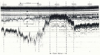
Fig. 11. Detail of the hanging dam of Figure 10 acquired with the 101C antenna unit.
Table II. Comparison between Radar and Drilling Data

The up-stream side of the open water in Figure 11 demonstrates the minimum ice thickness resolvable in the raw data produced by this antenna. The ice-surface and bottom reflections begin to merge at the right side of the open-water demarcation at a time difference of 3 ns or at about 0.14 m of ice. However, it is easy to trace the ice thickness to less than 0.05 m because the ice-bottom reflection is so much stronger than the surface reflection. The apparent difference in height between the water level and the adjacent ice surface is due to a lower flight altitude.
Figure 12 compares the ice thickness down-stream interpreted from the 101C radar profile with a drilling profile performed in the same vicinity on 15 April, 17 days after the radar profile with the 101C was performed. The discrepancy in time and positioning precludes the possibility of good correlation. However, the drilling confirmed the existence of solid ice at least 1.6 m thick in this area.

Fig. 12. Comparison between the drilling (solid line - performed 17 days after the radar survey) and radar surveys of ice thickness in the frazil dam.
Figure 13 summarizes ice depth for the entire 30 km 3102 profile as compiled from a hand digitization of 830 points. Measurements were made at ten equally spaced points between minute marks. The average depth of 0.83 m is typical of sections showing coherent surface and bottom returns. Thicknesses less than 0.2 m are associated with the open-water section of Figure 10 or 11.

Fig. 13. Statistics of the Yukon River ice thickness compiled from 830 digitized points along the entire profile.
Several stations along the Yukon River were sampled for ice and snow depth on 1 April, 5 days after the radar survey. The probability that we landed within 50 m of the station marking on the record is estimated at less than 10%, especially in the cross-river direction. Nevertheless, a comparison between radar and drilling data is attempted in Table II. The radar statistics for each station were compiled from points along the profile within an estimated 50 m of the station. The drilling data in Table II do not include the many measurements of snow density that were made at each station. Generally, snow density ranged between 0.16 and 0.39 Mg/m3, with an average of 0.22 Mg/m3 which, according to Reference CummingCumming (1952), has a dielectric constant of about 1.3, sufficient to cause the first reflection seen on the records, but low enough not to mask the ice reflections.
The comments under the drilling section in Table II reveal the wide variation of situations encountered. Two holes (all holes at each station were spaced 7–10 m apart) at station 13 revealed 64 cm of clear (“black”) ice, which corresponds excellently with the radar average of 66 cm. A third hole, however, revealed 109 cm of hard (no water) frazil ice and dirt. Similarly, two holes at station 27:00 revealed mostly hard frazil ice and dirt, while a third revealed clear ice to 79 cm. Most interesting were two holes at station 35:00, which revealed a section consisting of 79 cm of clear ice, 25 cm of liquid water, and then hard frazil ice to a depth beyond 180 cm, the length of our augers. A third hole in this area showed 107 cm of clear ice, 25 cm of water, and 36 cm of hard frazil ice. The radar data (Fig. 10) near this station gave depths of 110–130 cm, with much incoherency in the bottom returns.
Limited data were obtained at the remaining three stations (39:00, 62:17, 74:00) because the dirt (some pebbles) in the ice had ruined the cutters on our augers and core barrel, and the last three holes were done with great effort. Therefore, the chance of sampling anywhere near the flight line was one-third of what it was for the first three stations. The comparison of averages at the bottom of Table II is probably the most significant entry. The worst agreement is at station 62:17, where the drilled depth is clearly out of the measured radar range. Fortunately, several crosssections were done near station 62 in an attempt to discover very thick ice on the south-east shore. One of these profiles, done right at station 62:17 (easily identified by an obvious landmark), is shown in Figure 14 and reveals a section where ice depth did range around the sampled depth of 58 cm.

Fig. 14. 3102 profile of a cross-section of the Yukon River at station 62:17 along with the ice thickness measured on this record. Values beyond 100 m are estimated from the record.
V. Summary, conclusions, and recommendations
Despite the limited Yukon River sampling, the general accuracy of the Yukon River survey and the statistics of the ice-thickness distribution presented are believed reliable because: (1) the ground truth obtained on lakes and on the Tanana River conformed to the radar interpretation; (2) the fresh-water solid ice formations encountered generally conformed to the smoothly layered idealizations desired for geophysical exploration systems whose interpretations are based on plane-wave theory; and (3) variable dielectric permittivities in the main body of the ice were highly unlikely for late March and were not evidenced by any internal reflections within the ice sheets. A variable εr would be a factor for surveys conducted in late spring when ice begins to melt internally.
Surface roughness was a strong factor in deteriorating data quality. Any surface roughness would scatter the transmitted energy and make the bottom appear rough, whether or not the bottom is actually smooth. In no instance were temporally coherent bottom returns associated with incoherent surface returns, which is entirely logical. The presence of some coherency and hyperbolic shaping in the bottom returns, however, suggests that much of the bottom contouring could be recovered by migrating the data. This should be a simple procedure as there is only one layer present for which the dielectric constant should not vary significantly from 3.2.
The solid ice-thickness variations seen in the Tanana River cross-sections were well within the resolution capabilities of the radar so long as low altitude and low speed could be maintained. In neither of these cross-sections was there any evidence of the large top-to-bottom frazil dams that existed. Subsequent examination of these dams showed a high enough percentage of water to cause strong reflections from beneath the solid ice and little chance of penetration. The Yukon River profile at higher altitude and speed gave strong evidence of the presence of frazil ice because of its solid nature, the incoherency of the bottom returns, and their variable echo-delay times. The incoherency resulted from the greater lateral range of sensitivity inherent with higher altitudes, and demonstrates that “as low as possible” may not always be best.
Our future plans are to utilize a satellite-based positioning system and a lower-frequency antenna capable of giving water depth. The latter is entirely feasible to about 10 m depth with present, commercially available antennae operating between 50 and 100 MHz. Such a system would allow mapping of the presence of brash or wet frazil deposits, but probably not their depth due to the unknown dielectric permittivity. Deconvolution schemes based on Wiener least-squares filtering are presently being applied to facilitate automatic data interpretation.
Acknowledgements
This research was supported by the River Ice Management Program of Civil Works Project CWIS 32284 at the U.S. Army Cold Regions Research and Engineering Laboratory. We are indebted to Mr B. Brockett and Mr E. Chacho of CRREL, who developed the cross-sections in Figure 4 and assisted in the Yukon River drilling.


