2.1. Model design

Three airfoil models were used in the current experiment: a rigid airfoil, an airfoil with a flexible membrane skin on the leeward surface (hereinafter referred to as a flexible airfoil) and an airfoil with a flexible membrane skin actuated by MFCs on the leeward surface (hereinafter referred to as an actively controlled airfoil). The cross-section of the rigid airfoil was a complete NACA0012 airfoil. The flexible and the actively controlled airfoils were based on the NACA0012 airfoil with a cavity ranging from 16.7 % to 83.3 % of the chord length on the airfoil leeside. The cavity was deep to the airfoil centreline to ensure enough space to cover the flexible membrane skin. The cross-section shape of the flexible and the actively controlled airfoils is shown in figure 1. For all the three models, the chord lengths (c) and effective spans were 120 mm and 455 mm, respectively, resulting in aspect ratios of approximately 3.8. The models were made of stainless steel. The flexible skin adopted the same transparent thermoplastic polyurethanes (TPU) material as our previous single-layer membrane airfoil experiments (He & Wang Reference He and Wang2020; He et al. Reference He, Guo and Wang2022). The Young's modulus, thickness and density of the membrane were E = 31.2 MPa, t_m = 0.2 mm and ρ_m = 1.1 g cm⁻³, respectively. Small steps of ~5 mm width and ~0.2 mm depth were reserved before and behind the cavity to paste double-sided adhesive tape and fix the flexible membrane above the cavity. The chordwise length of the cavity and the original length of the membrane were 80 mm, while the length of the line connecting the front and rear of the cavity (d) was approximately 80.1 mm. To ensure the initially flatness of the membrane, a pre-strain of approximately 0.13 % was applied $({\varepsilon _0} = (80.1 - 80)/80 \approx 0.13\,\%)$. In addition, the joints between the membrane and the airfoil should be as smooth as possible.

Figure 1. Structural diagram of the actively controlled airfoil.

Figure 1 illustrates the detailed structure of the actively controlled airfoil. A complete active controller was installed in the middle of the model. The active controller consisted of MFC actuators and carbon-fibre substrate. To ensure the active control has sufficient spanwise length, inspired by Debiasi et al. (Reference Debiasi, Bouremel, Lu and Ravichandran2013) and Jones et al. (Reference Jones, Debiasi, Bouremel, Santer and Papadakis2015), three identical MFC actuators (Smart Material M5628-P1) were used in the experiment. For each actuator, the actuation length, actuation width and overall width were 56 mm, 28 mm and 35 mm, respectively. The capacitance was C = 8.7 nF, and the average shape variable per volt was approximately 0.75 μm m⁻¹. Due to the advantages of high strength, small mass and ease to process, a carbon-fibre sheet with 230 mm length, 60 mm width and 0.2 mm thickness was selected as the substrate. The MFC actuators and substrate were firmly bonded with epoxy in a vacuum. As shown by the locally enlarged view in figure 1, the active controller was pasted beneath the flexible membrane through double-sided tape to form a ‘sandwich’ structure of membrane–MFC actuator–carbon-fibre substrate. Along the airfoil section, the leading- and trailing-edges of the active controller were approximately 5 mm and 65 mm away from the front of the cavity, respectively. Along the spanwise direction, three MFC actuators were arranged on the substrate with equal distance. The active controller was in parallel with the span, while its central axis was located at the mid-span. The area ratio of the active controller to the entire flexible membrane skin was approximately 38 %. The model was installed vertically in the wind tunnel, so the effect of the active controller gravity on the membrane deformation could be ignored.

Moreover, it is seen from figure 1 that the direction of incoming flow is from left to right. Therefore, the three-dimensional coordinate system can be defined. The x-axis is the streamwise direction parallel to the incoming flow; the z-axis is the spanwise direction of the model; the y-axis is perpendicular to the x–z plane and referred to as the vertical direction. The origin of the x–y plane (cross-section plane) is located at the leading-edge when α = 0°. As a result, the trailing-edge non-dimensional coordinates normalized by the chord length are fixed as (1,0) at any α.

2.2. Measurements

The present experiment was carried out in the low-speed, open-loop and closed-jet D6 wind tunnel at Beijing University of Aeronautics and Astronautics (BUAA). The experimental set-up is shown in figure 2. The airfoil model passed through the upper wall of the wind tunnel and was vertically installed in the test section. End plates were installed approximately 20 mm away from the upper and lower walls to reduce the boundary layer influence of the wind tunnel wall on the flow around the airfoil. Accordingly, the effective span of the model was 455 mm. The free stream velocity U_∞ was 7.5 m s⁻¹, resulting in the Reynolds number based on c of Re = 6 × 10⁴. The free stream turbulent intensity Tu was less than 0.3 % at the current operating condition.

Figure 2. Set-up of the present experiment.

First, the aerodynamic forces of each model were measured in the wide range of α = −5° to 30° in 1° increments. As shown in figure 2, aerodynamic forces were determined by a six-component load cell (ATI-Mini40) with a range of 20 N (calibration standard SI-20-1). The load cell was factory-calibrated such that the static forces obtained were already corrected. In addition, the dynamic force calibration of the load cell at O(10¹–10²) Hz was conducted in the current study. Details can be found in Appendix A. The load cell and the airfoil model were connected through an aluminium clamp. All of them were connected to an electric turntable through an insulated connector. The electric turntable was finally fixed on a steel support which stretched across but not contacted with the wind tunnel. All connectors could ensure the connection stiffness. The insulated connector could eliminate the influence of static electricity generated by the motor of the electric turntable on the load cell. The positioning accuracy of the electric turntable was ±0.01°, so the angles of attack could be precisely adjusted. It was reported that the accuracy of load cell holds only if the measurements are made within 60 s due to the sensor output drift (Bleischwitz Reference Bleischwitz2016). To ensure reliable measurements, two wind-off tare points were obtained before and after each measurement, and then averaged as the baseline. Hence, the load repeatability error was less than ±5 × 10⁻³ N. Each measurement point was the average of data sampled at 4 kHz over 45 s, which could meet the requirements of high time-resolution and ergodicity. The sampling number of forces was approximately 1.8 × 10⁵. The resolution of the x- and y-axes of the load cell was 5 × 10⁻³ N. The uncertainties of force measurements in the current study are given here.

The lift and drag coefficients are calculated by

(2.1)\begin{gather}{C_l}\textrm{ = }\frac{L}{{{\textstyle{1 \over 2}}{\rho _a}U_\infty ^2S}},\end{gather}

(2.2)\begin{gather}{C_d}\textrm{ = }\frac{D}{{{\textstyle{1 \over 2}}{\rho _a}U_\infty ^2S}},\end{gather}

where L is the lift, D is the drag, and ρ_a and S are the air density and wing area, respectively. The uncertainty of C_l originating from both the uncertainties of L and U_∞ could be estimated by the uncertainty propagation formula (Kline & McClintock Reference Kline and Mcclintock1953):

(2.3) \begin{align}\begin{aligned} \varepsilon ({C_l}) & = \sqrt {{{\left( {\dfrac{{\partial {C_l}}}{{\partial L}}} \right)}^2}{\varepsilon ^2}(L) + {{\left( {\dfrac{{\partial {C_l}}}{{\partial {U_\infty }}}} \right)}^2}{\varepsilon ^2}({U_\infty })} \\ & = \sqrt {{{\left( {\dfrac{2}{{{\rho _a}U_\infty^2S}}} \right)}^2}{\varepsilon ^2}(L) + {{\left( {\dfrac{{ - 4L}}{{{\rho _a}U_\infty^3S}}} \right)}^2}{\varepsilon ^2}({U_\infty })} \\ & = \dfrac{2}{{{\rho _a}U_\infty ^2S}}\sqrt {{\varepsilon ^2}(L) + {{\left( {\dfrac{{2L}}{{{U_\infty }}}} \right)}^2}{\varepsilon ^2}({U_\infty })}, \end{aligned}\end{align}

where ε denotes the uncertainties. In the current study, ε(L) and ε(D) are the resolution of the load cell (5 × 10⁻³ N), and ε(U_∞) is the uncertainty of the Pitot tube used in the wind tunnel (~1 % U_∞ = 0.075 m s⁻¹). Accordingly, dividing (2.3) by (2.1) gives the relative uncertainty of C_l:

(2.4)\begin{equation}\frac{{\varepsilon ({C_l})}}{{{C_l}}} = \sqrt {\frac{{{\varepsilon ^2}(L)}}{{{L^2}}} + {{\left( {\frac{2}{{{U_\infty }}}} \right)}^2}{\varepsilon ^2}({U_\infty })} .\end{equation}

Similarly, the relative uncertainty of C_d is

(2.5)\begin{equation}\frac{{\varepsilon ({C_d})}}{{{C_d}}} = \sqrt {\frac{{{\varepsilon ^2}(D)}}{{{D^2}}} + {{\left( {\frac{2}{{{U_\infty }}}} \right)}^2}{\varepsilon ^2}({U_\infty })} .\end{equation}

It can be found that the uncertainties of lift and drag coefficients are related to specific values of forces, and thus they should be different. For the actively controlled airfoil at α = 12° in the current study, $\varepsilon ({C_l})/{C_l}$ and $\varepsilon ({C_d})/{C_d}$ are 2.0 % and 3.6 %, respectively.

Then, in specific cases, time-resolved synchronous measurements on forces, two-dimensional (2-D) deformations and flow fields were carried out. As displayed in figure 1, particle image velocimetry (PIV) measurement was undertaken at section A after preliminary tests. Section A was close to the mid-span of the model but avoided the middle MFC body, so that the damage to MFC caused by high temperature under direct laser irradiation could be avoided. In PIV measurement, dioctyl sebacate (DEHS) droplets with mean diameter $d_p \approx 1\;{\rm \mu}\mathrm{m}$ were generated and seeded by a MicoVec aerosol generator as tracer particles. According to Timpe et al. (Reference Timpe, Zhang, Hubner and Ukeiley2013), the relaxation time ${\tau_r} = d_p^\textrm{2}(\rho_p/18\ \mathrm{\mu})$ can determine how quickly the tracer particles can follow the flow under Stokes flow assumption for very small diameter spheres. Here, $\rho_p$ is the particle density. The relaxation time in this study was equal to 3 × 10⁻⁶ s (~300 kHz), which was enough for resolving different flow scales. As presented in figure 2, illumination of the desired plane was achieved by a Beamtech Vlite-Hi-527-30 high-speed double-pulsed laser with a minimum energy of 30 mJ pulse⁻¹ at 1 kHz frame rate. The laser pulse duration at the full-width-half-maximum (FWHM) location was less than 200 ns. The thickness of the laser sheet was approximately 1.5 mm. Because the steel models were opaque, the laser sheet could only illuminate the flow field above the airfoil leeside and in the wake. A Pco.dimax HS4 high-speed CMOS camera was arranged at the bottom to capture PIV image pairs. Thus, the instantaneous particle distributions and section deformations could be simultaneously recorded. The sampling frequency of image pairs was set to 800 Hz, also satisfying the requirements of time resolution. Due to the storage limitation of the camera, 8333 image pairs (namely 8333 snapshots of velocity fields) with the sampling time of approximately 10 s could be captured at one time. The diameters of most particles were approximately three pixels, so the peak-locking effect was negligible (Christensen Reference Christensen2004). The streamwise maximum stretching of particle images was less than two pixels, so its influence on the identification of particle image displacement should be small. The main PIV parameters are listed in table 1. The recorded 12-bit raw particle images were processed based on the multi-pass iterative Lucas–Kanade algorithm (MILK) accelerated by graphic processing units (GPUs) to obtain original velocity fields (Champagnat et al. Reference Champagnat, Plyer, Le Besnerais, Leclaire, Davoust and Le Sant2011; Pan et al. Reference Pan, Xue, Xu, Wang and Wei2015). The interrogation window size was set to 32 × 32 pixels with a 75 % overlap. The approach of recognizing membrane deformation was elaborated in previous studies (He & Wang Reference He and Wang2020; Hu, Feng & Wang Reference Hu, Feng and Wang2020; He et al. Reference He, Guo and Wang2022). It can provide a pixel accuracy of 0.08 % c (0.1/120 ≈ 0.08 %) with a resolution of 0.1 mm pixel⁻¹, the same as the magnification of PIV.

Table 1. PIV parameters.

The synchronous measurements on forces, deformations and flow fields were controlled by a MicroVec Micropulse-725 synchronizer. The four channels of the synchronizer were linked to a data acquisition card, a high-speed camera and the two heads of the laser. The deformation and flow field information were contained in the particle images simultaneously, so they were strictly synchronized. The synchronization of forces, deformations and flow fields was realized by controlling the accordant starting time of these three samplings. By setting the pulse period, pulse delay and other parameters of the synchronizer, the sampling frequency and straddle time could be adjusted. The control error of the synchronizer was less than 0.25 ns, which was high enough for accurate synchronous control.

2.3. Control parameters

In the experiment, the active control was realized by piezoelectric MFC actuators. The MFC is a layered, planar actuation device that employs rectangular cross-section, unidirectional piezoceramic (PZT) fibres embedded in a thermosetting polymer matrix. This active, fibre-reinforced layer is then sandwiched between copper-clad Kapton film layers that have an etched interdigitated electrode pattern (Bilgen et al. Reference Bilgen, Kochersberger, Diggs, Kurdila and Inman2007). It has both direct and inverse piezoelectric effects. This study used the inverse piezoelectric effect of the MFC. The working principle is shown in figure 3. Under applied voltage signals, the MFC actuator will undergo extension or contraction, driving the substrate to bend and resulting in the periodically transverse membrane vibration.

Figure 3. Working principle of the MFC actuator (Feng et al. Reference Feng, Guo, Wang and Xu2022).

To reinforce the 2-D property of the active controller along the spanwise direction, the three MFC actuators shown in figure 1 were connected into the circuit in parallel. It could be observed from a monitoring UNI-T UPO2104CS oscilloscope that the phase difference of the three electrical signals was zero. The quasi-2-D property at the actively controlled region is further verified in Appendix B. The maximum and minimum operating voltages of the MFC actuators were +1500 V and −500 V, respectively. To ensure sufficient control intensity and safety, a RIGOL DG1022U function/arbitrary waveform generator was used to produce a sinusoidal voltage signal with bias. The valley value of the signal was −1.5 V and the peak value was +7.5 V. The voltage signal from the generator was further amplified by a Smart Material HVA 1500/50-4 high-voltage amplifier with a voltage gain of 200 V/V. Consequently, the voltage signal could be amplified into the range of −300 V to +1500 V to actuate MFC to work normally. Meanwhile, the actuation signal was real-time monitored by the oscilloscope. The final actuation voltage signal is

(2.6)\begin{equation}V(t) = {\textstyle{1 \over 2}}{V_{pp}}\sin (2{\rm \pi}{f_a}) + {V_{bias}},\end{equation}

where V_pp is the peak-to-peak value of actuation voltage, f_a is the actuation frequency and V_bias is the bias voltage of +600 V. According to Leighton & Huang (Reference Leighton and Huang2010), the MFC actuator bonded to the substrate can be treated as a ‘piezoelectric unimorph beam’ structure. In this structure, the bending displacement is linearly correlated to the applied electric field. Accordingly, the mean deformation of the actuators is correlated to the mean actuation voltage (essentially the bias voltage). Actuation voltage and actuation frequency are two important control parameters in this experiment. By changing their amplitudes, the active control of flexible membrane could be realized. Furthermore, two non-dimensional parameters can be obtained, namely, reduced frequency ${f^ + } = {f_a}c/{U_\infty }$ and reduced voltage ${V^ + } = {V_{pp}}/{({V_{pp}})_{max}}$. The reduced voltage is non-dimensionalized by the maximum peak-to-peak value of ${({V_{pp}})_{max}} = 1800\;\textrm{V}$. The control parameters are listed in table 2.

Table 2. Control parameters.

The control effects of ${f^ + }$ and ${V^ + }$ on the lift coefficients are shown in figure 4. Rigid and flexible cases are also plotted. In figure 4(a), ${V^ + }$ is fixed to 1, and ${f^ + }$ is 0.16, 1.60, 2.88 and 3.52. It can be found that when α < 10° and α > 14°, there is little difference between the actively controlled airfoil at each ${f^ + }$. When 10° ≤ α ≤ 14°, the lift coefficient and stall angle of attack of the actively controlled airfoil gradually increase with the increase of ${f^ + }$. In figure 4(b), ${f^ + }$ is fixed to 1, and ${V^ + }$ is 0.33, 0.67 and 1. The control effect of ${V^ + }$ is similar to that of ${f^ + }$. When 10° ≤ α ≤ 14°, the lift coefficient and stall angle of attack of the actively controlled airfoil gradually increase with the increase of ${V^ + }$. Therefore, when the control parameters are $({f_a},{V_{pp}}) = (220,1800)$, the active control has the best effect on improving the aerodynamic characteristics. The corresponding non-dimensional parameters are $({f^ + },{V^ + }) = (3.52,1)$. Moreover, when ${V^ + } = 0.33$, the aerodynamic performance of the actively controlled airfoil is slightly worse than the flexible airfoil, implying that the active actuation is not necessarily better than passive flow control in certain cases.

Figure 4. Effects of control parameters on lift coefficients. (a) Effects of reduced frequency; (b) effects of reduced voltage.

3.1. Mean aerodynamics

The aerodynamic coefficient curves of each model are first shown in figure 5. Except for the rigid and flexible airfoils, two parameter combinations of $({f^ + },{V^ + }) = (0,0)$ (without actuation case) and $({f^ + },{V^ + }) = (3.52,1)$ (best actuation case) for the actively controlled airfoil are compared. The black dashed line in figure 5(a) is the lift curve C_l = 2α for linearized thin-airfoil theory. As presented in figure 5(a), when α ≤ 5°, the lift coefficients of each airfoil are basically consistent with the thin-airfoil theory, which verifies the accuracy of force measurement. With the increase of α, the lift variation of these models is different individually. When α < 0°, the lift curves of the rigid airfoil, flexible airfoil and actively controlled airfoil collapse well. When 0° ≤ α ≤ 10°, four models present a competitive relationship in lift characteristics, but the overall lift difference is small. When α > 10°, obvious difference appears in the lift curves. For the rigid airfoil, the stall angle of attack is α = 10°. After that, the rigid airfoil will gradually suffer stall at α > 10°, where the lift coefficient will decrease sharply. However, for the actively controlled airfoil, the lift will further increase at α > 10°. Compared with the rigid airfoil, the stall α of the actively controlled airfoil is delayed from 10° to 12°. The maximum lift coefficient is increased from 0.780 to 0.844 with an increment of 8.2 %. At α = 12°, the lift coefficient increment from 0.664 to 0.844 is the largest, which is 27.1 %. In short, the above results indicate that through proper active control, the maximum lift of the airfoil can be improved and the stall can be delayed. In addition, it can be found in figure 5(a) that the lift of each airfoil after stall (α > 15°) will further increase, which is consistent with previous studies on low-Reynolds-number wings (Michos, Bergeles & Athanassiadis Reference Michos, Bergeles and Athanassiadis1983; Zhou et al. Reference Zhou, Alam, Yang, Guo and Wood2011; Guo et al. Reference Guo, He, Wang and Wang2021).

Figure 5. Aerodynamic coefficients. (a) Lift curves; (b) drag curves.

The drag curves of the airfoils are displayed in figure 5(b). When α ≤ 10°, the drag coefficients of the rigid and the actively controlled airfoils are basically the same. When α > 10°, the drag coefficient of the rigid airfoil increases sharply due to stall, while the drag coefficient of the actively controlled airfoil does not increase significantly until α = 12°. It means that the active control can achieve lift-enhancement and drag-reduction simultaneously in the angle of attack range where the rigid airfoil encounters stall.

In addition, it can be discovered in figure 5 that there is little difference between the aerodynamic performance (both the lift and the drag) of the flexible and rigid airfoils. The without actuation case $({f^ + },{V^ + }) = (0,0)$ is also close to the former two airfoils. These findings indicate that the passive control method by simply changing the flexibility of the upper airfoil surface can hardly improve the aerodynamic characteristics, which is totally different from the previous research on a single-layer membrane airfoil (Rojratsirikul et al. Reference Rojratsirikul, Wang and Gursul2009; Bleischwitz et al. Reference Bleischwitz, de Kat and Ganapathisubramani2017; He & Wang Reference He and Wang2020; He et al. Reference He, Guo and Wang2022).

Figure 6 shows the lift-to-drag ratios and polar curves of the models, wherein the lift-to-drag ratios are exhibited in figure 6(a). When α < 10°, the maximum lift-to-drag ratio of the rigid airfoil is higher than that of the actively controlled airfoil, indicating that the active control cannot improve the maximum lift-to-drag ratio before stall. When 10° ≤ α ≤ 14°, active control can greatly improve the lift-to-drag ratio of the rigid airfoil in the post-stall state due to its advantages of lift-enhancement and drag-reduction. At α = 11° and 12°, the increments of the lift-to-drag ratios of the actively controlled airfoil are 126 % and 121 % compared with the rigid airfoil, respectively. With the further increase of α (α ≥ 15°), the lift-to-drag ratio of each model is completely consistent, indicating the active control no longer has advantages. Additionally, the polar curves are shown in figure 6(b). It is also found that the actively controlled airfoil has the best aerodynamic performance at approximately the first peak of lift curve. In a word, the best application environment of the actively controlled airfoil is at 10° ≤ α ≤ 14°, where the rigid airfoil is in the post-stall state. By active control, the disadvantage of premature stall of the rigid airfoil is overcome, and better aerodynamic performance is obtained.

Figure 6. Relationship between lift and drag. (a) Lift-to-drag ratios; (b) polar curves.

3.2. Active control efficiency

According to Seifert (Reference Seifert2015), the active control efficiency can be evaluated by the first, second and fourth Aerodynamic Figures of Merit (AFM), which are

(3.1)\begin{gather}AFM1 = \frac{{{U_\infty }{L_a}/({U_\infty }{D_a} + {P_a})}}{{{{(L/D)}_b}}},\end{gather}

(3.2)\begin{gather}AFM2 = \frac{{{U_\infty }({L_a} - {W_a} + {W_s})/({U_\infty }{D_a} + {P_a})}}{{{{(L/D)}_b}}},\end{gather}

(3.3)\begin{gather}AFM4 = \frac{{{U_\infty }{D_a} + {P_a}}}{{{U_\infty }{D_b}}},\end{gather}

where AFM1 evaluates the efficiency of boundary layer separation control as well as lift-to-drag ratio enhancement, AFM2 considers the weight for flight based on AFM1 and AFM4 evaluates the efficiency of drag reduction. The subscript ‘b’ is the baseline case (rigid airfoil) and the subscript ‘a’ is the actuation case (actively controlled airfoil). Here, W_a is the total weight of the actuation system and W_s is the weight savings due to active control, and P_a is the total power consumption of the actuator. Referring to Bai et al. (Reference Bai, Zhou, Zhang, Xu, Wang and Antonia2014), P_a is related to the dissipation of the PZT actuators operated at an actuation frequency f_a and peak-to-peak value of actuation voltage V_pp, which are calculated by

(3.4)\begin{equation}{P_a} = 2{\rm \pi} N{f_a}C\tan (\delta) {\left( {\frac{{{V_{pp}}}}{{2\sqrt 2 }}} \right)^2},\end{equation}

where N = 3 is the total number of MFC actuators, C = 8.7 nF is the capacitance of the MFC and tan(δ) = 2 % is the dissipation factor of the PZT material used in the MFC (Nováková & Mokrý Reference Nováková and Mokrý2011). According to (3.4), P_a equals to 0.29 W for the best actuation case $({f_a},{V_{pp}}) = (220,1800)$ in this study.

In (3.1), when AFM1 > 1, the separation control is efficient for additional power consumption. While in (3.3), when AFM4 < 1, the drag reduction is efficient for additional power consumption. As a result, AFM1 > 1 and AFM4 < 1 are preferred for efficient active control. The variations of AFM1 and AFM4 from α = 2° to 30° in the current study are shown in figure 7. It can be found that the two points α = 11° and 12° are in the efficient active control region. Although the drag of the actively controlled airfoil is lower than that of the rigid airfoil at α = 10° (see figure 5b), the additional power consumption makes AFM4 > 1, which is inefficient for drag reduction.

Figure 7. Variations of AFM1 and AFM4 from α = 2° to 30° for the actively controlled airfoil.

In addition, it is true that the active control system can bring additional weight, but it depends on the applications. It was reported by Seifert (Reference Seifert2015) that the active control system could replace or reduce the weight of an existing systems, such as simplified high-lift configurations. The weight for flight could be saved as long as W_a < W_s for AFM2 in (3.2).

3.3. Flow statistical characteristics

PIV measurement was further conducted at different angles of attack. The time-averaged streamlines are displayed in figure 8. The leeward skins of flexible and actively controlled airfoils are illustrated by time-averaged membrane deformations. The red dashed curves in figures 8(d) and 8(e) denote the positions where the mean streamwise velocity component equals to 0 $(\langle U\rangle = 0)$, which represent the scale of the leeward separation region (Munday & Taira Reference Munday and Taira2018). It can be seen from figure 8(a–c) that before the occurrence of stall (α ≤ 10°), the time-averaged flow is attached to the leeside of the airfoils without separation. Therefore, each airfoil shows similar aerodynamic characteristics in figure 5(a) when α ≤ 10°. However, in figure 8(d), there are large recirculation regions over the rigid and flexible airfoils, indicating the flow around them encounters severe separation at α = 12°. The scales of the two separation regions are approximately identical, implying the passive deformation in this experiment has little effect on the flow separation over the airfoil. This phenomenon explains why the difference between the aerodynamic characteristics of the flexible and rigid airfoils is small, as shown in figure 5, and further elucidates that simply changing the flexibility of the upper airfoil surface can hardly improve the aerodynamic characteristics. The flow around the actively controlled airfoil is completely different from the former two airfoils. The separation region over the airfoil totally disappears by active control and the streamlines pass smoothly along the airfoil surface. When α increases to 20° in figure 8(e), the three airfoils have large and similar recirculation regions, which means that both the passive and active control in the current study can hardly suppress the flow separation and improve the aerodynamic performance at high angle of attack. To sum up, the lift-enhancement and drag-reduction of the actively controlled airfoil in the range of 10° ≤ α ≤ 14° is attributed to the effective suppression of flow separation over the leeward surface.

Figure 8. Time-averaged streamlines at different angles of attack: (a) α = 0°; (b) α = 4°; (c) α = 10°; (d) α = 12°; (e) α = 20°. The leeward skins of flexible and actively controlled airfoils are illustrated by time-averaged membrane deformations. The scales of separation regions are illustrated by the line of $\langle U\rangle = 0$, depicted as the red dashed curves.

According to the mean aerodynamics in figure 5 and the time-averaged streamlines in figure 8, the maximum lift-enhancement for the actively controlled airfoil is achieved at α = 12°, so the statistical characteristics of the flow field around airfoils are analysed at α = 12° and shown in figure 9. Figure 9(a) exhibits the non-dimensional time-averaged velocity $(\sqrt {{{\langle U\rangle }^2} + {{\langle V\rangle }^2}} /{U_\infty })$ contours as well as the time-averaged streamlines. The good effect of active control on suppressing flow separation can be further observed. Figure 9(b) illustrates the non-dimensional time-averaged vorticity $(\langle \omega \rangle c/{U_\infty })$ contours. The negative and positive regions represent the clockwise and counterclockwise vorticity in the leading- and trailing-edge shear layers, respectively. Above the airfoil surface, the vorticity of the rigid and flexible airfoils is concentrated in the separated shear layer, while the vorticity of the actively controlled airfoil is close to the airfoil surface, which further indicates the flow separation is suppressed by the actively controlled airfoil.

Figure 9. Flow statistical characteristics at α = 12°. (a) Time-averaged velocity and streamlines; (b) time-averaged vorticity; (c) turbulent kinetic energy. Each row includes different models.

Moreover, the non-dimensional turbulent kinetic energy (TKE, $\langle {u^{\prime2}} + {v^{\prime2}}\rangle /U_\infty ^2$) is presented in figure 9(c). TKE characterizes the fluctuation characteristics of the flow around the airfoil. Similar to the vorticity distribution in figure 9(b), TKE of the former two airfoils is concentrated in the separated shear layer, while TKE of the actively controlled airfoil is close to the airfoil surface. Compared with the former two airfoils, the actively controlled airfoil has a slightly higher TKE level in the near-wall region. Nevertheless, the strong unsteadiness in the recirculation region is significantly weakened due to the suppression of flow separation, resulting in an obvious reduction in the overall fluctuation level. Figures 9(b) and 9(c) further show the boundary layer range over the actively controlled airfoil at α = 12°. The boundary layer thickness is calculated by integrating spanwise vorticity along the wall normal direction (more details will be described in § 4.1.2). The near-wall TKE is shown to be almost completely distributed in the leeward surface boundary layer, which means that the fluctuations in the boundary layer caused by active control are closely related to the separation suppression and aerodynamic performance improvement. The fluctuations of active control intensify the momentum mixing in the boundary layer, reduce the inverse pressure gradient, suppress the flow separation and finally improve the lift coefficient at post-stall angles of attack. This is similar to the lift-enhancement mechanism of passive vibration of single-layer membrane airfoil (He et al. Reference He, Guo and Wang2022).

4.1. Spectral characteristics

The spectral characteristics of the unsteady aerodynamics and fluid–structure interaction of the actively controlled airfoil are first studied. The spectra of instantaneous aerodynamic forces are obtained by fast Fourier transformation (FFT). The spectra of global membrane vibrations and flow fields are obtained by Fourier mode decomposition (FMD) proposed by Ma et al. (Reference Ma, Feng, Pan, Gao and Wang2015). The main principle of FMD is given here. For the selected flow fields, single-point discrete Fourier transform (DFT) is first applied to velocity data at every mesh node to get a Fourier mode matrix c_k,

(4.1)\begin{equation}{\boldsymbol{c}_k} = \frac{1}{N}\sum\limits_{n = 0}^{N - 1} {{\boldsymbol{F}_n}\,{\textrm{e}^{ - \textrm{i}(2{\rm \pi} k/N)n}}} ,\end{equation}

where N = 8333 is total sampling number of image pairs, F_n is the original velocity complex matrix where the real and imaginary parts are streamwise and vertical velocities, respectively. The global power spectrum density (PSD_k) is further defined as

(4.2)\begin{equation}PS{D_k} = \left\|{\frac{{2N|{\boldsymbol{c}_k}{|^2}}}{{{\rm \pi}{f_s}}}} \right\|,\end{equation}

where $||\cdot ||$ is the Frobenius norm, f_s is the sampling frequency. For the membrane vibrations, DFT of membrane displacements at 300 chordwise equidistant positions is similarly conducted through (4.1) and the PSD of global membrane vibrations is then obtained by (4.2).

The frequency spectra of the actively controlled airfoil at α = 12° are summarized in figure 10. The frequency is non-dimensionalized as the Strouhal number $St = fc/{U_\infty }$. In figure 10, St ₁ = 1.76, St ₂ = 3.52 and St ₃ = 5.28 correspond to 110 Hz, 220 Hz and 330 Hz, respectively. Here, St ₂ and St ₃ are the second and third harmonics of St ₁. According to the spectra of aerodynamic forces in figure 10(a), there are two peaks St ₁ and St ₃ in the lift spectrum. The PSD of the St ₃ peak is slightly higher than the St ₁ peak, so the dominant frequency of the lift is St ₃. Different from the lift, the dominant frequency of the drag is St ₁. Comparing the spectra of global membrane vibrations (figure 10b) and flow fields (figure 10c), it can be found that their dominant frequencies are both St ₁. The PSD of the two harmonic peaks (St ₂ and St ₃) decreases in turn. In sum, the drag, membrane vibrations and flow fields are completely coupled with the same dominant frequency of St ₁. Although the dominant frequency of lift is St ₃ instead of St ₁, the PSD peaks of the two frequencies are close, which means that the instantaneous lift is determined by both St ₁ and St ₃.

Figure 10. Spectral characteristics of the actively controlled airfoil at α = 12°. (a) Spectra of the aerodynamic forces; (b) spectrum of global membrane vibrations; (c) spectrum of global flow fields. Seven frequency bands in the membrane spectrum are defined by a frequency splitting vector for the following mPOD process.

Figures 11(a) and 11(b) show the energy distributions and Fourier modes based on vertical velocity components corresponding to the three frequencies at α = 12°. The three disturbances with different frequencies are shown to induce coherent structures continuously convecting downstream in the leeward surface boundary layer. Meanwhile, according to the energy distribution, the disturbances of St ₁ and St ₂ are mainly concentrated on the airfoil leeward surface. The disturbance of St ₃ is concentrated both on the airfoil leeward surface and in the wake. Next, the frequency response characteristics of membrane and flow fields under active control will be analysed.

Figure 11. Energy distributions and Fourier modes based on vertical velocity components corresponding to the three frequencies at α = 12°. (a) Energy distributions; (b) Fourier modes. The frequencies from left to right are St ₃, St ₂ and St ₁, respectively.

4.1.1. Frequency response characteristics of membrane vibrations

It is an interesting behaviour in figure 10(b) that the dominant frequency of membrane vibrations is half of the reduced frequency, namely, $S{t_1} = 0.5{f^ + }$. To determine the underlying mechanism, frequency response characteristics of membrane vibrations are investigated at reduced frequencies from 0.37 to 3.73. Membrane deformations of the actively controlled airfoil are measured at wind-off and wind-on. First, the chordwise vibration amplitudes y_std (standard deviations of the vertical membrane displacements) are shown in figure 12. It can be seen in figure 12(a–d) that the number of y_std peaks at wind-on is the same as that at wind-off, which means that the vibration behaviour of the membrane is similar at wind-on and wind-off when ${f^ + } < 3$. However, in figures 12(e) and 12( f), y_std has three peaks at wind-off, but it only has two peaks at wind-on. It means that the vibration behaviour at wind-on changes abruptly when ${f^ + } > 3$.

Figure 12. Chordwise vibration amplitudes: (a) ${f^ + } = 0.37$; (b) ${f^ + } = 1.55$; (c) ${f^ + } = 2.42$; (d) ${f^ + } = 2.90$; (e) ${f^ + } = 3.15$; ( f) ${f^ + } = 3.73$. The black and magenta curves indicate the wind-off and wind-on cases, respectively.

Furthermore, the spectral characteristics are analysed. The dominant frequencies of membrane vibrations at different reduced frequencies at wind-on are displayed in figure 13. When ${f^ + } < 3$, the dominant frequency of membrane vibration is the same as the reduced frequency, that is, $S{t_1} = {f^ + }$. However, when ${f^ + } > 3$, the dominant frequency of membrane vibration is half of the reduced frequency, that is, $S{t_1} = 0.5{f^ + }$. Thus, the half-frequency lock-in phenomenon at ${f^ + } > 3$ is newly discovered in this paper.

Figure 13. Relationship between dominant frequencies of membrane vibrations and reduced frequencies at wind-on.

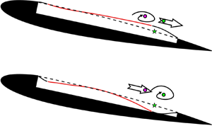
The reason for the half-frequency lock-in is then investigated based on instantaneous membrane vibrations at ${f^ + } = 3.52$. Due to the strong periodicity of the active control, the instantaneous membrane vibration signals are adopted as the reference for the phase-averaging process. Here, the instantaneous membrane vibrations in the time series of 8333 snapshots are cross-correlated with the membrane vibration at the basic instant (snapshot No. 1000 is arbitrarily selected). The obtained correlation coefficient signal is then low-pass filtered and the information of the dominant vibration frequency (St ₁) is retained. Hilbert transformation is then employed to get phase information (Pan, Wang & Wang Reference Pan, Wang and Wang2013). The phase-averaged membrane vibrations are plotted in figure 14. As shown, the active controller could incline and bend in a vibration cycle, driving the membrane to deform and vibrate.

Figure 14. Phase-averaged membrane vibrations of the actively controlled airfoil at α = 12°.

However, the membrane vibrations in figure 14 seem to be complicated. Hence, multi-scale proper orthogonal decomposition (mPOD), a data-driven reduced-order method proposed by Mendez, Balabane & Buchlin (Reference Mendez, Balabane and Buchlin2019), is used to analyse the frequency response characteristics of membrane vibrations. The mPOD combines multi-resolution analysis (MRA) with a standard POD. For MRA, the mPOD can split the correlation matrix into the contribution of different scales by a user-defined frequency splitting vector F_V, retaining non-overlapping portions of correlation spectra. Then, standard POD is conducted upon these scales to extract their optimal eigenbases, which can be kept mutually orthogonal and finally assembled into a single mPOD basis. Briefly, mPOD provides an excellent compromise between energy optimality and spectral purity.

As shown in figure 10(b), seven frequency bands in the membrane spectra are defined by a frequency splitting vector F_V = [100, 120, 210, 230, 320, 340] Hz to contain the three characteristic frequencies for mPOD. The corresponding non-dimensional frequency splitting vector is St_V = [1.60, 1.92, 3.36, 3.68, 5.12, 5.44]. The wind-off and wind-on cases are both investigated. Figure 15 presents the mode shape and spectrum of the first mPOD mode at wind-off. Clearly, this mode is the ‘bending’ mode of the active controller with a dominant frequency of St ₂ = 3.52. This frequency is equal to the reduced frequency ${f^ + }$, which means that the bending mode is directly caused by the actuation. However, the most energetic mode at wind-on (shown in figure 16a) is the ‘inclining’ mode with a dominant frequency of St ₁ = 1.76. In contrast, the bending mode becomes less energetic at wind-on (shown in figure 16c). Thus, the shift of the dominant vibration mode from bending to inclining is the reason for half-frequency lock-in when ${f^ + } > 3$.

Figure 15. mPOD results of the actively controlled airfoil at wind-off. (a) Mode shape of the first mPOD mode; (b) spectrum of the first mPOD mode.

Figure 16. mPOD results of the actively controlled airfoil at wind-on. (a) Mode shapes of the first two mPOD modes; (b) spectra of the first two mPOD modes.

4.1.2. Frequency response characteristics of flow fields

In figure 11, the disturbances of St ₁, St ₂ and St ₃ are concentrated on the airfoil leeward surface, which may be related to the natural frequencies of the local shear layer. According to Ho & Huerre (Reference Ho and Huerre1984), Hsiao, Liu & Shyu (Reference Hsiao, Liu and Shyu1990), Wu et al. (Reference Wu, Lu, Denny, Fan and Wu1998) and Bohnker & Breuer (Reference Bohnker and Breuer2019), there exist the most unstable frequencies in the shear layer. The shear layer is sensitive to the disturbance of these frequencies, resulting in the roll-up and shedding of leading-edge vortices. The most unstable frequency is referred to as the natural frequency of the shear layer and denoted by $f_{shear}^0$. The non-dimensional natural frequency is defined as

(4.3)\begin{equation}S{t_{shear}} = \frac{{f_{shear}^0\theta }}{{({U_\infty } + 0)/2}}\textrm{ = }\frac{{2f_{shear}^0\theta }}{{{U_\infty }}},\end{equation}

where θ is the momentum thickness which can be obtained by boundary layer thickness. The boundary layer thickness δ is defined as the wall-normal distance between the airfoil surface and the boundary layer edge $(Y_N^{edge})$. The location of $Y_N^{edge}$ is at the separatrix between the boundary layer flow and the inviscid free stream (Wang & Wang Reference Wang and Wang2021). However, the standard boundary layer assumption (the velocity at the boundary layer edge equals to 0.99U_∞) remains invalid due to the curved airfoil surface. Instead, as proposed by Marxen et al. (Reference Marxen, Lang, Rist, Levin and Henningson2009), the pseudo velocity attained by wall-normal integration of time-averaged spanwise vorticity $\langle \omega \rangle$ is used to determine $Y_N^{edge}$:

(4.4)\begin{equation}{u_{pseudo}} = \int_0^{Y_N} {\langle \omega \rangle \,\textrm{d}{Y_N}} ,\end{equation}

where $Y_N^{}$ is the wall-normal coordinate with the origin on the airfoil surface. Here, $Y_N^{edge}$ is defined as the position where the variation of ${u_{pseudo}}$ converges along the wall-normal direction. Then the displacement thickness δ* and momentum thickness θ are calculated by the following equations:

(4.5)\begin{gather}\delta^\ast= \int_0^{Y_N^{edge}} {\left( {1 - \frac{{{u_{pseudo}}({Y_N})}}{{{u_{pseudo}}(Y_N^{edge})}}} \right)\,\textrm{d}{Y_N}} ,\end{gather}

(4.6)\begin{gather}\theta = \int_0^{Y_N^{edge}} {\left( {1 - \frac{{{u_{pseudo}}({Y_N})}}{{{u_{pseudo}}(Y_N^{edge})}}} \right)\frac{{{u_{pseudo}}({Y_N})}}{{{u_{pseudo}}(Y_N^{edge})}}\,\textrm{d}{Y_N}} .\end{gather}

The streamwise variation of δ, δ* and θ of the actively controlled airfoil at α = 12° is illustrated in figure 17(a). Here, ${x_\delta }$ is the streamwise locations of the boundary layer edge. As shown, the three thicknesses gradually increase along the streamwise direction. For the natural frequency of the shear layer, $S{t_{shear}}$ is empirically determined to be approximately 0.034 for a laminar flow and between 0.044 and 0.048 for a turbulent flow (Ho & Huerre Reference Ho and Huerre1984; Wu et al. Reference Wu, Lu, Denny, Fan and Wu1998). Because of the large disturbance of actuation, the flow state over the airfoil surface should be turbulent. Thus, the natural frequencies of the shear layer can be calculated via substituting the θ values obtained by (4.6) into (4.3). Then the streamwise variation of $f_{shear}^0$ is identified and shown in figure 17(b). The current PIV sampling frequency is 800 Hz. To meet the requirements of Nyquist sampling theorem, the ceiling of the y-axis in figure 17(b) is limited to 400 Hz. Due to the inverse proportional relationship with θ, $f_{shear}^0$ gradually transits from high frequency to low frequency along the streamwise direction. Figure 17(b) further shows the frequencies of St ₃, St ₂ and St ₁ (as shown by three horizontal dashed lines). There are three intersection parts between these frequencies and the upper and lower limits of $f_{shear}^0$. By selecting the medians of these parts, the streamwise locations corresponding to the three disturbing frequencies can be obtained, which are ${x_\delta }/c\sim 0.37$, 0.45 and 0.65. It means that the three frequencies are likely to be amplified near these locations. In figure 17(c), the amplification locations of different disturbances are marked along the wall-normal direction in the flow field. Their relative positions with the airfoil can be seen more clearly, which are helpful to the following analyses of the unsteady coupling process.

Figure 17. Frequency response characteristics of flow field. (a) Streamwise variation of boundary layer thicknesses of the actively controlled airfoil at α = 12°; (b) streamwise variation of natural frequencies of the shear layer; (c) amplification locations of different disturbing frequencies. The background contour is the time-averaged vorticity.

4.2. Unsteady coupling process

After obtaining the Fourier modes for specific frequencies, the flow fields can be reconstructed from the modes with certain frequency bands based on the FMD method (Wang et al. Reference Wang, Feng, Wang and Li2018; Wang, Wang & Kim Reference Wang, Wang and Kim2019). The reconstructed flow fields can ensure the time localization in the current study, that is, the occurrence of a characteristic flow event in the reconstructed flow fields is at the same time as the original flow fields. Taking advantage of this feature, the original flow fields are decomposed and reconstructed by FMD, and the unsteady aerodynamics and fluid–structure coupling process corresponding to different frequencies are analysed. The frequency resolution of FMD in this study is Δf = 800/8333 = 0.096 Hz with a non-dimensional resolution of ΔSt = 1.5 × 10⁻³. For the frequencies of St ₁, St ₂ and St ₃, three narrow bands of St ₁ ± 2ΔSt, St ₂ ± 2ΔSt and St ₃ ± 2ΔSt are selected for reconstruction. As a result, three reconstructed flow fields are obtained, which are denoted as $St_1^{recon}$, $St_2^{recon}$ and $St_3^{recon}$.

4.2.1. Coupling between instantaneous lift and flow fields

In this section, we first conduct cross-correlation between instantaneous lift and flow fields to analyse their relationship. The instantaneous lift fluctuation ${C^{\prime}_l}$ and the global instantaneous swirl strength ${\lambda _{ci}}$ at every mesh node in the flow fields are selected as the correlation signals. Here, ${\lambda _{ci}}$, defined as the imaginary part of the complex eigenvalues of the velocity gradient tensor, is a vortex identification criterion and can distinguish the real vortical structures from the strong background shear flow. The ${\lambda _{ci}}$ values can characterize the strength of local vortical structures (Zhou et al. Reference Zhou, Adrian, Balachandar and Kendall1999). The cross-correlation equation is as follows:

(4.7)\begin{equation}{R_{{{C^{\prime}}_l}{\lambda _{ci}}}}(x,y,t) = \frac{{\langle {{C^{\prime}}_l}(t){\lambda _{ci}}(x,y,t)\rangle }}{{{\sigma _{{{C^{\prime}}_l}}}{\sigma _{{\lambda _{ci}}}}}}.\end{equation}

The spatial cross-correlation between two signals can be reflected by (4.7) with zero-time lag. The correlation results are displayed in figure 18, wherein, figure 18(a) is the correlation contour between lift fluctuation and original flow field. Figures 18(b)–18(d) show the correlation contours between lift fluctuation and three reconstructed flow fields $St_1^{recon}$, $St_2^{recon}$ and $St_3^{recon}$, respectively. It can be seen from figure 18(a) that the correlation regions between ${C^{\prime}_l}$ and ${\lambda _{ci}}$ are mainly located inside the boundary layer. The correlation coefficient presents alternately positive and negative distributions over the airfoil leeward surface and in the wake. The minimum (R = −0.40) and maximum (R = 0.62) correlation coefficients over the leeward surface appear at points P1 and P2, respectively. Points P1 and P2 are respectively situated upstream and downstream of the point L1 with maximum vibration amplitude in the membrane. They are also at the vertical positions with maximum TKE (the black thin curve indicates the maximum TKE positions along the streamwise direction). Due to the negative clockwise vorticity over the airfoil leeward surface, the negative correlation at P1 means that when the clockwise vortex with the largest vorticity appears at P1, the lift reaches the maximum; when the vortex moves away from P1, the lift reduces to the minimum. In contrast, the positive correlation at P2 means that when the clockwise vortex with the largest vorticity appears at P2, the lift reduces to the minimum; when the vortex leaves P2, the lift reaches the maximum. Comparing the correlation contours between lift fluctuation and reconstructed flow fields, it can be found that the lift has obvious correlation with the reconstructed flow fields $St_1^{recon}$ (figure 18b) and $St_3^{recon}$ (figure 18d). However, the correlation level with $St_2^{recon}$ (figure 18c) is very low. These results indicate that the flow structures of St ₁ and St ₃ have significant effects on the lift, while the flow structures of St ₂ have little influence. They further confirm the finding in figure 10 that the frequency of St ₂ has negligible contribution to the PSD of the lift. In addition, by comparing figures 18(b) and 18(d), a surprising phenomenon is discovered near L1 that there are two regions with high correlation levels at around P1 and P2, indicating that these two regions over the airfoil have the most significant influence on the instantaneous lift. The swirl strength of clockwise vortices in these regions is closely related to the lift.

Figure 18. Global cross-correlation coefficient contours between the instantaneous lift fluctuation ${C^{\prime}_l}$ and swirl strength ${\lambda _{ci}}$ at every mesh node in the flow field at α = 12°. (a) ${C^{\prime}_l}$ versus original flow field; (b) ${C^{\prime}_l}$ versus $St_1^{recon}$; (c) ${C^{\prime}_l}$ versus $St_2^{recon}$; (d) ${C^{\prime}_l}$ versus $St_3^{recon}$.

Moreover, the correlation concentration regions can reflect the location of the flow structures. In figures 18(b)–18(d), the amplification positions of three different disturbances St ₁, St ₂ and St ₃ are marked along the wall-normal direction (consistent with figure 17c). It is shown that the three disturbances are amplified near each unstable position in the flow field, triggering the flow instability and causing the roll-up, downstream convection and shedding of coherent structures. So far, the generation mechanism of the coherent structures over the airfoil leeward surface in this study is verified by the shear layer theory. Here, St ₁ and its harmonics are coupled with the theoretical natural frequencies of the leading-edge shear layer. Coherent structures with different scales and frequencies are generated near the most unstable positions. Combined with figure 9(c), the generation of these flow structures is accompanied by the enhancement of momentum mixing in the leeward surface boundary layer close to the wall. Finally, the flow structures help to suppress flow separation and improve the aerodynamic performance at post-stall angles of attack.

The aerodynamic forces, membrane vibrations and flow fields are averaged according to the phases in § 4.1.1 to obtain the final phase-averaged signals. As shown in figure 19, the curves on the left display time histories of the phase-averaged force fluctuation signals as well as phase-averaged vibration signal at L1. The contours on the right show the ${\lambda _{ci}}$ distributions of phase-averaged flow fields. From top to bottom are the original and reconstructed flow fields. Because of the very low correlation level of the second harmonic in figure 18(c), the second harmonic reconstructed flow field is not shown in figure 19.

Figure 19. Phase-averages forces, membrane vibrations and flow fields at α = 12°. (a) Φ = 100° with the maximum lift; (b) Φ = 270° with the minimum lift. The curves on the left display time histories of the phase-averaged force fluctuation as well as phase-averaged vibration signals at L1. For clarity, the drag fluctuation ${C^{\prime}_d}$ and vibration L1-y′ signals are multiplied by factors of 4 and 50, respectively. The contours on the right shows the ${\lambda _{ci}}$ distributions of phase-averaged flow fields. Phase-averaged membrane deformations with amplitudes amplified by a factor of five are appended for better display.

It can be seen from the curves in figure 19 that in a membrane vibration cycle with the dominant frequency St ₁, the lift has a global maximum at Φ = 100° and a global minimum value at Φ = 270°. The phase difference between them is ΔΦ ≈ 180°, namely a half cycle. In addition, there are two other local maxima at Φ ≈ 220° and 350° as well as two local minima at Φ ≈ 40° and 170°. The results indicate that the lift has the spectral features of St ₁ and St ₃ simultaneously. The drag has only a maximum at Φ ≈ 70° and a minimum at Φ = 270° due to its dominant frequency St ₁. These conclusions are consistent with the spectra of lift and drag in figure 10(a). In addition, it is presented that lift and drag reach their global minima simultaneously, which means that although the active control can successfully achieve the goal of lift-enhancement and drag-reduction, the largest reduction of instantaneous drag is accompanied by the cost of the lowest instantaneous lift.

The instantaneous flow fields are given in figure 19 at the phases where the lift reaches the global maximum (figure 19a) and minimum (figure 19b). Intuitively, at Φ = 100° with the maximum lift, there is a vortex concentrated at P1. At Φ = 270° with the minimum lift, a larger vortex is concentrated at P2. This further elucidates the distribution of correlation coefficients in figure 18 from the perspective of instantaneous vortical structures.

Furthermore, the phase-averaged time histories of ${C^{\prime}_l}$, L1-y′, and instantaneous ${\lambda _{ci}}$ values at P1 and P2 (denoted as P1-${\lambda _{ci}}$ and P2-${\lambda _{ci}}$) in a membrane vibration cycle are given in figure 20(a). First, at Φ = 100° with the maximum lift, the swirl strength of the reconstructed flow fields $St_1^{recon}$ and $St_3^{recon}$ at P2, denoted as $\textrm{P2 - }\lambda _{ci}^{St_1^{recon}}$ and $\textrm{P2 - }\lambda _{ci}^{St_3^{recon}}$, both are equal to zero. At Φ = 270° with the minimum lift, $\textrm{P2 - }\lambda _{ci}^{St_1^{recon}}$ and $\textrm{P2 - }\lambda _{ci}^{St_3^{recon}}$ drop to near the global minima corresponding to the largest clockwise swirl strength. Second, the variation of lift is found to be in-phase with $\textrm{P2 - }\lambda _{ci}^{St_3^{recon}}$. The three minima of $\textrm{P2 - }\lambda _{ci}^{St_3^{recon}}$ are respectively located at Φ ≈ 40°, 160° and 280°, which are basically consistent with the instantaneous lift. However, the three minima of $\textrm{P2 - }\lambda _{ci}^{St_3^{recon}}$ are very close, but the three minima of lift show different magnitudes. It means that even if the lift is determined by St ₁ and St ₃ (see figure 10a), the effects of the two frequencies are different. Here, St ₁ determines the phases of global maximum and minimum of lift, while St ₃ determines the phases of local maxima and minima of lift. When the effects of the two frequencies are superposed, the lift can reach its global maximum and minimum. Therefore, $\textrm{P2 - }\lambda _{ci}^{St_1^{recon} + St_3^{recon}}$ is obtained by linear superposition of $\textrm{P2 - }\lambda _{ci}^{St_1^{recon}}$and $\textrm{P2 - }\lambda _{ci}^{St_3^{recon}}$, whose variation is also shown by the green curve in figure 20(a). Amazing similarity can be found between $\textrm{P2 - }\lambda _{ci}^{St_1^{recon} + St_3^{recon}}$ and the lift where the variation of lift follows well with $\textrm{P2 - }\lambda _{ci}^{St_1^{recon} + St_3^{recon}}$ regardless of the phases of global or local minima, indicating a close in-phase relationship. Since the correlation level between ${\lambda _{ci}}$ and ${C^{\prime}_l}$ at P2 in figure 18(a) is higher, P1 is not selected here.

Figure 20. Relationship between signals at α = 12°. (a) Phase-averaged time histories of ${C^{\prime}_l}$, L1-y′, $\textrm{P1 - }{\lambda _{ci}}$ and $\textrm{P2 - }{\lambda _{ci}}$ in a membrane vibration cycle; (b) correlation coefficients with phase lags.

Based on figure 20(a), phase lead-lag properties of two signals can be derived from cross-correlation in figure 20(b). The maximum correlation coefficient between lift and drag fluctuations is 0.80 with a phase difference of ΔΦ = 0°, that is, the lift and drag are essentially in-phase. The maximum correlation coefficients of ${C^{\prime}_l}$ versus $\textrm{P2 - }\lambda _{ci}^{original}$ and ${C^{\prime}_l}$ versus $\textrm{P2 - }\lambda _{ci}^{St_1^{recon} + St_3^{recon}}$ are close, with phase differences of ΔΦ = 0° and −4°, respectively, indicating that they are all in-phase. The two correlation curves are similar, which proves the feasibility of using the linearly superposed swirl strength $\textrm{P2 - }\lambda _{ci}^{St_1^{recon} + St_3^{recon}}$. Compared with $\textrm{P2 - }\lambda _{ci}^{original}$, the linearly superposed $\textrm{P2 - }\lambda _{ci}^{St_1^{recon} + St_3^{recon}}$ can eliminate the influence of other irrelevant frequencies (such as the little correlation of ${C^{\prime}_l}$ versus $\textrm{P2 - }\lambda _{ci}^{St_2^{recon}}$ in figure 20b) on the lift, and can reflect the variation of lift more intuitively.

Here, the reason why the instantaneous swirl strength at P2 affects the lift is also explained. The flow fields at Φ = 100° and Φ = 270°, corresponding to figures 19(a) and 19(b), are respectively exhibited in figures 21(a) and 21(b) by streamlines. Referring to the research of Jones, Yao & Allan (Reference Jones, Yao and Allan2006) on circulation-control wings, the streamline deflection is related to lift-enhancement through the augmentation of the circulation around the wing. In this experiment, an upstream point S (x/c = 0.1, y/c = 0.245) with a normal height from the local airfoil surface of 0.15 mm is selected. From the point S, we release two streamlines in figures 21(a) and 21(b) simultaneously. The streamlines at the two phases are shown with red lines in the figures. They are further put together for comparison in figure 21(c). It can be found that at Φ = 270°, the streamline deflects upward at P2. It is because the instantaneous swirl strength of the vortex at P2 is the largest and the local streamline is lifted-up by the strong vortex. At the downstream of P2, the streamline at Φ = 270° is always higher than Φ = 100°. Additionally, the blue curves in figure 21(c) represent the slope variation of the two streamlines along the streamwise direction. The most obvious difference in the slope curves is still at point P2: at Φ = 270°, the absolute value of streamline slope decreases obviously, which also reflects the upward deflection of the streamline at P2. In the wake, the slopes of the two streamlines (linear fitted) at Φ = 100° and Φ = 270° remain unchanged and equal to −0.068 and −0.056, respectively. Consequently, at Φ = 270°, the upward deflection of the streamline reduces the clockwise circulation around the airfoil and further reduces the lift. At Φ = 100°, the more downward streamline deflection leads to the larger clockwise circulation around the airfoil and higher lift. The above conclusions can still be obtained by comparing other streamlines near the airfoil surface in figures 21(a) and 21(b). It should be noted that the explanation about figure 21 is based on quasi-steady assumption, in which the instantaneous lift is determined by the instantaneous circulation (Theodorsen Reference Theodorsen1935; Gao Reference Gao2012). The additional unsteady lift caused by virtual mass force is ignored because the vibration velocity of the membrane on the airfoil surface is one order of magnitude smaller than the free stream velocity. Therefore, through the analysis of the instantaneous streamline deflection, the influence of instantaneous swirl strength at P2 on the lift is reasonably explained.

Figure 21. (a) Flow field at Φ = 100° with the maximum lift; (b) flow field at Φ = 270° with the minimum lift; (c) comparison of selected streamlines and their slopes.

4.2.2. Coupling between membrane vibrations and flow fields

Subsequently, the membrane vibrations are considered to investigate the unsteady aerodynamics and fluid–structure coupling characteristics. For the unsteady membrane vibrations, the point L1 with maximum vibration amplitude is located closely between P1 and P2, so the variation of L1-y′ has a significant impact on the instantaneous swirl strength of P1 and P2. The phase difference between ${C^{\prime}_l}$ and L1-y′ in figure 20(b) is ΔΦ = 56°. In other words, both the instantaneous lift fluctuation and the swirl strength at P2 lag behind the membrane vibration signal at L1. According to the time histories in figure 20(a), the maximum of L1-y′ is located at Φ = 50°. At this phase, a local bulge appears around L1 in the membrane, hindering the downstream development of the local shear layer. After some time, vorticity will accumulate around the upstream point P1 (absolute value of $\textrm{P1 - }\lambda _{ci}^{St_1^{recon} + St_3^{recon}}$ is the largest at Φ = 80°–100°), while the vorticity around the downstream point P2 will convect away ($\textrm{P2 - }\lambda _{ci}^{St_1^{recon} + St_3^{recon}}$ is 0 at Φ = 100°). In contrast, the minimum of L1-y′ is located at Φ = 200°. At this phase, a local dent appears around L1 in the membrane, no longer hindering the development of the shear layer. Therefore, the vorticity around P1 will gradually convect downstream ($\textrm{P1 - }\lambda _{ci}^{St_1^{recon} + St_3^{recon}}$ is 0 at Φ = 250°– 290°), while strong vorticity will accumulate around P2 (absolute value of $\textrm{P2 - }\lambda _{ci}^{St_1^{recon} + St_3^{recon}}$ is near the largest at Φ = 270°). To intuitively display the above events, figure 22 shows the coupling relationship between membrane vibrations and flow structures. The fluid–structure coupling events after the appearance of local membrane bulge at Φ = 50° (figure 22a) and dent at Φ = 200° (figure 22b) are described.

Figure 22. Sketch of fluid–structure coupling relationship at α = 12°. (a) Fluid–structure coupling events after the appearance of local membrane bulge at Φ = 50°; (b) fluid–structure coupling events after the appearance of local membrane dent at Φ = 200°. Phase-averaged membrane deformations with amplitudes amplified by a factor of five are appended for better display.

So far, a close in-phase relationship between instantaneous lift fluctuation and linearly superposed swirl strength of the vortex at the P2 point is found above. The coupling mechanism between membrane deformation and vortices is also expounded. The unsteady coupling process can be then described as follows. The periodic occurrences of the local membrane bulge and dent around the maximum vibration amplitude location affect the instantaneous swirl strength of flow structures. The local swirl strength further influences the deflection of the local streamlines. Finally, the variations of circulation around the airfoil and the instantaneous lift are determined.