


1. INTRODUCTION
In this paper we use laser ablation-inductively coupled plasma-mass spectrometry (LA-ICP-MS) to measure sodium (Na), calcium (Ca) and iron (Fe) from three glacial age ice archive sections of the Siple Dome-A core (SDMA, Fig. 1). Resulting ultra-high resolution 121 µm sampling yields an average of 62 samples a−1 for the sections under study, providing sub-seasonal characterization of atmospheric circulation proxies and precipitation changes such as large storm events. For the first time at this depth in the SDMA core, we are able to annually date the record adding information to the current depth/age scale that has until now relied primarily on methane tie points to annually dated Greenland ice cores.
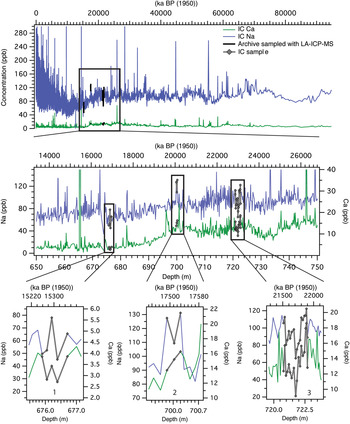
Fig. 1. Top time series – Original Siple Dome soluble calcium and sodium based on ion chromatography (IC). Middle and bottom time series – zoomed in views showing the three sections investigated in this study. Original IC sampling resolution is 16 cm for sections 1 and 2, and 11 cm for section 3 (Mayewski and others, Reference Mayewski2012).
2. METHODS
We utilize the Climate Change Institute's W.M. Keck Laser Ice Core Facility's LA-ICP-MS system for the ultra-high resolution glaciochemical analysis presented in this study following techniques presented by Sneed and others (Reference Sneed2015) and applications presented by Mayewski and others (Reference Mayewski, Sneed, Birkel, Kurbatov and Maasch2013). Components include a Thermo Element 2 ICP-MS coupled to a New Wave UP-213 laser system and the Sayre Cell™, a cryocell chamber designed to seal a 1 m ice core from the surrounding air, while maintaining a uniform temperature of −15°C and a 121 µm sampling resolution (Sneed and others, Reference Sneed2015). To calculate glaciochemical concentrations measured by LA-ICP-MS, a calibration technique using both liquid and frozen standards is used (Sneed and others, Reference Sneed2015). The SDMA ice archive sections used in this study are ~3 cm × 3 cm rods. Prior to analysis, the surface of the ice is scraped using a Lie Nielson stainless-steel blade to ensure a contaminant-free surface. The sample is then transferred into the Sayre Cell™ for analysis. We were able to sample ~180.28 cm of ice in this study, equating to 90 163 individual sample levels for Fe, Ca and Na. It was not possible to sample the selected archives continuously because the SDMA ice core is now over two decades old, and some of the ice is too fractured on the surface for sampling reliably by LA-ICP-MS. An airtight seal over the ice is required by the laser ablation system for the Argon carrier gas to transfer the ablated ice material into the ICP-MS, and the presence of any fractures interferes with the maintenance of the airtight seal. We measured Na, Ca and Fe from individual ablated lines along the surface of the ice core, to guarantee the necessary sample volume for analyses (Sneed and others, Reference Sneed2015).
3. RESULTS AND DISCUSSION
3.1. Sample intervals for climate snapshot analysis
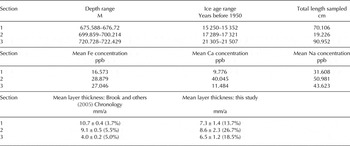
Table 1 below shows information regarding depth range, ice age range, length of ice sampled, mean annual layer thickness and mean concentrations of the three sections sampled in the SDMA archive. The SDMA ice archives sampled were chosen to investigate snapshots of late glacial ice constrained by the availability of fracture free, LA-quality ice for sampling. To calculate the mean annual layer thickness of each section of ice, we assumed that the non-sampled intervals had the same mean annual layer thickness as the sampled section.
Table 1. Information on the three sections sampled: depth range, Ice Age range (using the Brook and others, Reference Brook2005 depth/age model top depth for the ice sample in this study and then annual layer counting results in this study), total length sampled, mean concentrations of glaciochemistry measured and resulting mean annual layer thickness results with uncertainties from Brook and others (Reference Brook2005) and this study
3.2. Comparison of LA-ICP-MS with original ion chromatography (IC) results
Figure 2 shows the LA-ICP-MS 121 µm data with a highly smoothed (200 point binomial smooth) version compared with the original SDMA IC samples (11–16 cm mean sampling resolution). The sample smoothing is chosen primarily for ease of viewing. There is some agreement between LA-ICP-MS and IC results. However, IC and LA-ICP-MS results are not expected to be identical because the original IC record is a significantly coarser record, and IC measures only soluble chemistry, whereas LA-ICP-MS measures total element chemistry.
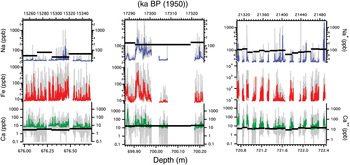
Fig. 2. laser ablation-inductively coupled plasma-mass spectrometry (LA-ICP-MS) data for section 1, 2 and 3 (left to right) with a 200-pt binomial smooth (raw 121 µm data plotted in background) compared with the original 16, 16 and 11 cm (left to right) mean sampling resolution of ion chromatography (IC) data (black dots). IC data from Mayewski and others (Reference Mayewski2012). Note: LA-ICP-MS data in this study is oversampled, and comparison of various timeseries smoothing parameters reveals that a 200-pt smooth does not detract from the overall trends in the dataset.
3.3. Glaciochemistry- sources and proxies for atmospheric circulation
To better understand the sources of the chemistry measured in this study, we calculated the seasalt (ss) and non-seasalt (nss) contributions using Nam as the conservative marine indicator. Seasalt sodium levels (ssNa) have been shown to decrease with distance from the ocean and elevation above sea level (Legrand and Mayewski, Reference Legrand and Mayewski1997; Bertler and others, Reference Bertler2005). The SDMA ice core IC Na+ results have been interpreted as inversely related to the Amundsen Sea Low pressure variability (Kreutz and others, Reference Kreutz2000) as well as to the ice dynamics/deglaciation of the Ross Sea Embayment (Mayewski and others, Reference Mayewski2012). Non-seasalt calcium (nssCa) is shown to be transported in the troposphere to the SD site by the austral circumpolar zonal westerlies, primarily in spring (Yan and others, Reference Yan, Mayewski, Kang and Meyerson2005). A climate proxy for nssCa-containing northerly air mass incursions into West Antarctica was developed based on the examination of 21 ITASE (International Trans Antarctic Scientific Expedition) ice core nssCa records, including SD (Dixon and others, Reference Dixon2011). Fe is primarily crustal in origin, transported from arid regions to oligotrophic ocean gyres, where it is an essential nutrient in phytoplankton productivity (Duce and Tindale, Reference Duce and Tindale1991; Raiswell and others, Reference Raiswell2006; Crusius and others, Reference Crusius2011).
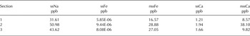
We found the vast majority of Fe to be of crustal origin (mean nssFe concentration is >99.9% of total) and a majority of the Ca to be crustal in origin (mean nssCa is 89.1% of total). The mean ss and nss contributions of the glaciochemistry measured are found in Table 2 below.
Table 2. Mean concentrations of non-seasalt (nss) and seasalt (ss) glaciochemistry contributions
3.4. Seasonal accumulation examination
The ultra-high sampling resolution of LA-ICP-MS makes it possible to extract information about relative seasonal accumulation rates. To do this we selected a 30 a sample size from each section. Because there are only 22 a counted in section 2, we used all years in section 2. For each annual layer counted in this study, we measure net winter accumulation and net summer accumulation using a 20-point binomial smooth. Net winter accumulation for a given year is measured as the distance between the rise of the deepest (earliest) local maximum in an element used to count a year and the fall of the shallowest (latest) local maximum in an element used to count the same year. Net summer accumulation for a given year is measured as the distance between the fall of the shallowest local maximum in an element used to count a year and the rise of the deepest local maximum in an element used to count the next year. Net accumulation values have not been corrected for layer thinning, thus do not represent values at the surface, but they still carry information relevant to relative changes. Results for net seasonal accumulation can be found in Table 3. The results show that the ratio of winter to summer precipitation (inferred from net winter and summer layer thicknesses) are relatively consistent (1.7, 1.3, and 1.6 for sections 1, 2 and 3 (~15.3, 17.3, 21.4 ka ago, respectively)). Notably the winter season is longer than the summer season in all sections, as would likely be expected in glacial age ice. This finding is consistent with a doubling of the summer season at the transition from the Younger Dryas cold period to the Holocene in LA-ICP-MS examination of the Greenland ice sheet project 2 (GISP2) (central Greenland) ice core (Mayewski and others, Reference Mayewski, Sneed, Birkel, Kurbatov and Maasch2013).
Table 3. Shown are mean net seasonal accumulation rates, inferred from summer and winter/spring layer thicknesses
3.5. Annual layer counting and comparison with SDMA depth/age model
The depth/age relationship for the SDMA ice core was developed from a variety of core parameters including: annual layering of visual stratigraphy; electrical conductivity; stable isotopes; major anions and cations; 10Be (Kreutz and others, Reference Kreutz2000; Taylor and others, Reference Taylor2004) plus ice dynamics modeling (Hamilton, Reference Hamilton2002). The depth/age relationship for the SDMA ice core from 8.3 ka to 57 ka was calculated by correlating methane and the isotopic composition of O2 in the SD ice core with that of GISP2 and Greenland ice core project (Brook and others, Reference Brook2005).
Previous studies show that heightened storm frequency during the winter and spring results in the transport of increased quantities of sea salts and dusts to the Antarctic ice sheet (Whitlow and others, Reference Whitlow, Mayewski and Dibb1992; Kreutz and others, Reference Kreutz1999). Given that seasonal storm structure (storm timing, magnitude, frequency) can vary annually, we assume that glaciochemical proxies used to understand seasonality, and hence annual layering, can also vary in seasonal timing. Therefore, dust and sea salt inputs to Antarctica are expected to vary during the winter and spring storm season and, as a consequence, glaciochemical proxies should not always be precisely in phase with each other. As such the ultra-high resolution sampling of LA-ICP-MS should reveal these differences.
Therefore, as a first approximation for identifying annual layers in this study, we define a winter/spring season for a given year as a ‘synchronous’ peak in all the three elements (Na, Ca and Fe) measured. ‘Synchronous’ troughs of background level concentrations are indicative of less stormy summers. We define ‘synchronous’ as peaks differing in depth by less than half the calculated mean annual layer thickness estimated using the Brook and others (Reference Brook2005) methane age control points.
Winters/springs, in which a single element peak is not present or is asynchronous with the other three element peaks do exist. This phenomenon could be explained most simply by either a change in the atmospheric transport pathway, by an atmospheric blocking pattern that prevents weather systems from reaching the ice core site, or by a change in the source area, or the seasonal input timing of the chemistry. Years counted that have two or fewer near-synchronous element peaks are noted as ‘less confident’ year picks and were used to develop our annual layer counting uncertainty, although, as noted these annual layers may be environmentally as significant. We define uncertainty as the percentage of less confident picks of all the annual layers counted in the study. In the 180.28 cm of ice sampled, we counted 249 a with an overall uncertainty of 19.2%. Examples showing annual layer picks for each of the three sections and their respective uncertainties are in Figure 3.
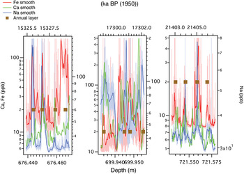
Fig. 3. Annual layer counting example taken from section 1, 2 and 3 (left to right, see Fig. 1 for locations), an ~3 cm section shown for sodium (blue), calcium (green) and iron (red). Brown boxes represent the center-point for annual layer picks, centered on winter/spring season maxima. 4 a are shown. A 200-point binomial smoothing is used for annual signal clarity. Raw 121 µm data for iron and sodium are shown as an example. Note: laser ablation-inductively coupled plasma-mass spectrometry (LA-ICP-MS) data in this study are oversampled, and comparison of various timeseries smoothing parameters reveals that a 200-pt smooth does not detract from the overall trends in the dataset.
The average annual layer thickness for each of the three sections sampled, and the model comparison, is found in Table 1. Given that the SDMA core from a depth of 514.8 m (gas age 8.3 ka) was dated by synchronizing methane signatures to annually dated Greenland core data (Brook and others, Reference Brook2005), we suggest annual counting to be a more accurate method to determine annual ice layer thicknesses on decadal scales. While methane is well-mixed globally it can also be argued that using methane tie points at the coarse resolution presented in Brook and others, Reference Brook2005 does not account for annual-decadal scale variability in snow accumulation, or the absence of years by wind scouring of snow. Only section 2 of this study is in exact agreement with the Brook and others, Reference Brook2005 depth/age model. If our estimated layer thicknesses based on annual layer counting are correct within the given uncertainty, this would suggest that the model's age of the ice near section 1 is slightly underestimated, and the age of the ice near section 3 is slightly overestimated.
4. CONCLUSION
The goal of this paper is to display the capabilities of ultra-high resolution LA-ICP-MS in the seasonal analysis of compressed sections of the SDMA ice core record. We show that the SDMA ice core record can be annually dated at a depth not previously possible using the original ~10–20 cm resolution. This resolution of record offers promise for future investigation of abrupt climate change events as demonstrated by Mayewski and others (Reference Mayewski, Sneed, Birkel, Kurbatov and Maasch2013) for the Younger Drays/Holocene abrupt climate transition in Greenland. The annual layer thickness results of this study are worth consideration for: future studies that use the SD ice core, further interpretations of the methane-based age scale in the deeper section of the SD record and in further understanding past changes to the West Antarctic ice sheet during the late glacial period.
ACKNOWLEDGEMENTS
This work was supported by National Science Foundation grants no. 1203640 and 1042883 to P. Mayewski. Data used in this paper are available at http://nsidc.org/data/nsidc-0636.


 Open access