


1. INTRODUCTION
There has been increasing interest in the use of underwater vehicles to explore and exploit the ocean, such as mine-hunting, target or animal tracking, disaster response, and oceanographic surveys (Moradi et. al., Reference Moradi, Rezazadeh and Ismail2012; Erol-Kantarci et. al., Reference Erol-Kantarci, Mouftah and Oktug2011; Waite, Reference Waite2002). Precise positioning of underwater vehicles is important for the safety and effectiveness of all these autonomous missions. However, the underwater environment is complex and access-constrained, presenting unique challenges to accurate positioning compared with land and air environments. In the underwater environment, the popular Global Positioning System (GPS) is not feasible due to the strong attenuation that the electromagnetic field suffers in water (Sukkarieh et. al., Reference Sukkarieh, Nebot and Durrant-Whyte1999; Yun et. al., Reference Yun, Bachmann, McGhee, Whalen, Roberts, Knapp, Healey and Zyda1999). Therefore, acoustic-based positioning systems have been sought in the past, including systems such as Long Baseline (LBL), Short Baseline (SBL), and Ultra-Short Baseline (USBL) (Tan et. al., Reference Tan, Diamant, Seah and Waldmeyer2011; Olson et. al., Reference Olson, Leonard and Teller2006; Kinsey et. al., Reference Kinsey, Eustice and Whitcomb2006).
In LBL, a set of three or more baseline transponders are deployed on the sea floor, and the positions of the transponders must be determined in advance (Jakuba et. al., Reference Jakuba, Roman, Singh, Murphy, Kunz, Willis, Sato and Sohn2008). In SBL, three or more transponders are mounted on a surface vessel and connected to a central control station. In both systems, a trilateration algorithm is used to estimate the target position (Tan et. al., Reference Tan, Zhong-ying and Hong-yuan2009). In USBL, a set of transponders assembled in a single device is installed on a support ship, and the target position is estimated by measuring the relative phases between the signals arriving at the transponders (Beaujean et. al., Reference Beaujean, Bon and An2010; Philips, Reference Philips2003). All of these systems have their merits and drawbacks. SBL and USBL require less infrastructure, but the positioning accuracy and the operational area are constrained. In comparison with SBL and USBL, LBL can achieve higher accuracy, but it has several shortcomings, e.g., requiring a long time for deployment and calibration, and a limited operating region.
Moving Long Baseline (MLBL) is a generalisation of LBL by replacing the pre-calibrated arrays of static transponders with self-calibrated and fully mobile transponders (Caiti et. al., Reference Caiti, Garulli, Livide and Prattichizzo2005; Alcocer et. al., Reference Alcocer, Oliveira and Pascoal2007). The absolute position of the target can be estimated by the Least Squares (LS) method based on the acoustic and GPS observations (Vaganay et. al., Reference Vaganay, Leonard, Curcio and Willcox2004; Kussat et. al., Reference Kussat, Chadwell and Zimmerman2005). In this way, the MLBL overcomes the shortcomings of LBL. In the past few years, many algorithms for efficient target position estimation have been proposed in the literature, such as Extended Kalman Filtering (EKF) (Olson et. al., Reference Olson, Leonard and Teller2006; Batista et. al., Reference Batista, Silvestre and Oliveira2014), Particle Filtering (PF) (Fox et. al., Reference Fox, Burgard, Kruppa and Thrun2000), and Maximum Likelihood Estimation (MLE) (Howard et. al., Reference Howard, Matark and Sukhatme2002).
In MLBL, the absolute position of the target is calculated by using the position measurements of the mobile buoys and the distance measurements between the target and the mobile buoys. The positioning error may arise from three factors, i.e., the position error of the mobile buoy relative to the earth reference frame, the traveling time error and the deviation of actual sound speed from the assumed sound speed (Moradi et. al., Reference Moradi, Rezazadeh and Ismail2012; Kinsey et. al., Reference Kinsey, Eustice and Whitcomb2006; Isik and Akan, Reference Isik and Akan2009; Liu et. al., Reference Liu, Chen, Zhong and Poor2010; Kaplan and Hegarty, Reference Kaplan and Hegarty2005; Teymorian et. al., Reference Teymorian, Cheng, Ma, Cheng, Lu and Lu2009). The distance between the mobile buoy and the target is calculated by the sound speed and the One-Way Travel Time (OWTT). Hence the positioning accuracy of the target is mainly affected by the position error of the mobile buoy and the distance error between the mobile buoy and the target. Considering that the positioning accuracy is only affected by the distance error, some researchers have found that the accuracy of the position estimates can be computed through the Cramer-Rao bound (CRB) and Fisher Information Matrix (FIM). Then the optimal geometry by minimizing the CRB or maximizing the FIM is provided (Van Trees, Reference Van Trees2004; Savvides et. al., Reference Savvides, Garber, Moses and Srivastava2005; Alcocer et. al., Reference Alcocer, Oliveira and Pascoal2006; Moreno-Salinas et. al., Reference Moreno-Salinas, Pascoal and Aranda2011; MartíNez and Bullo, Reference MartíNez and Bullo2006; Moreno-Salinas et. al., Reference Moreno-Salinas, Pascoal and Aranda2012; Purvis et. al., Reference Purvis, Astrom and Khammash2008; Oshman and Davidson, Reference Oshman and Davidson1999; Xu and Choi, Reference Xu and Choi2011). However, the position error of the mobile buoy is ignored. This work differs from the aforementioned approaches by considering that the positioning accuracy is affected by the distance error and the position error of the mobile buoy. According to the estimation theory, we propose a Positioning Accuracy Metric (PAM) to measure the positioning accuracy with the distance error and the position errors are also considered. We find that the positioning accuracy is related to the distance between the mobile buoy and the target. The optimal distance is determined by the depth of the target and the parameter of the distance error.
The remainder of the paper is organised as follows. Section 2 presents the mathematical model of MLBL. The PAM with the distance error and the position error considered is proposed in Section 3. Section 4 presents the optimal geometry and the optimal distance. Section 5 illustrates the simulation results. Finally, we conclude our work in Section 6.
2. MATHEMATICAL MODEL OF MLBL
As shown in Figure 1, the mobile buoys on the water surface are equipped with transponders, Differential GPS (DGPS), wireless communications, and the target is equipped with transponders. The position of the target is determined by the position measurements of the mobile buoys and the distance measurements between the target and each mobile buoy.

Figure 1. MLBL positioning system consists of four mobile buoys.
2.1. Kinematics model
As shown in Figure 2, consider an earth fixed reference frame {O}: = {x 0, y 0, z 0} with z = 0 on the water surface, and the z-axis pointing downward from the water surface. The coordinate of the target at stamp k is (x k, yk, zk).

Figure 2. The kinematics model of the target.
The kinematics model of the target is described as
 $$\left\{ {\matrix{ {x_{k + 1} = x_k + T_s v_{xk} = x_k + T_s v_k \cos \psi _k \cos \theta _k,} \cr {y_{k + 1} = y_k + T_s v_{yk} = y_k + T_s v_k \sin \psi _k \cos \theta _k,} \cr\hskip-30pt {z_{k + 1} = z_k + T_s v_{zk} = z_k + T_s v_k \sin \theta _k,} \cr}} \right.$$
where T s is the sampling period, v k is the velocity, ψ k is the yaw, θ k is the pitch. Suppose there are m mobile buoys on the water surface, their coordinates at stamp k are (x i,k, y i,k, z i,k), with z i,k = 0. The kinematics model of each mobile buoy is described as
 $$\left\{ {\matrix{ {x_{i,k + 1} = x_{i,k} + T_s v_{i,k} \cos \psi _{i,k},} \cr {y_{i,k + 1} = y_{i,k} + T_s v_{i,k} \sin \psi _{i,k},} \cr} \; \; i = 1,...,m} \right.,$$
where v i,k is the velocity, ψ i,k is the yaw.
2.2. Positioning model
Assuming that the positions of the mobile buoys and the distances between the target and each mobile buoy are known, the estimated position of the target (x k, yk, zk) should satisfy
 $$\left( {x_k - x_{i,k}} \right)^2 + \left( {y_k - y_{i,k}} \right)^2 + \left( {z_k - z_{i,k}} \right)^2 = r_{i,k}^2, i = 1,...,m.$$
As mentioned before, the mobile buoys are on the water surface with z i,k = 0, then we have
 $$2\left( {x_{i,k} - x_{\,j,k}} \right)x_k + 2\left( {y_{i,k} - y_{\,j,k}} \right)y_k = - r_{i,k}^2 + r_{\,j,k}^2 + x_{i,k}^2 + y_{i,k} ^2 - x_{\,j,k}^2 - y_{\,j,k}^2$$
where i ≠ j, x k and y k are unknown variables to be estimated. The positioning model can be expressed as
 $${\bi AX} = {\bi B},$$
where
 $${\bi A} = \left[ {\matrix{ {2\left( {x_{1,k} - x_{2,k}} \right)} & {2\left( {y_{1,k} - y_{2,k}} \right)} \cr {2\left( {x_{2,k} - x_{3,k}} \right)} & {2\left( {y_{2,k} - y_{3,k}} \right)} \cr \vdots & \vdots \cr {2\left( {x_{m - 1,k} - x_{m,k}} \right)} & {2\left( {y_{m - 1,k} - y_{m,k}} \right)} \cr {2\left( {x_{m,k} - x_{1,k}} \right)} & {2\left( {y_{m,k} - y_{1,k}} \right)} \cr}} \right],{\bi X} = \left[ {x_k, y_k} \right]^T, $$
and
 $${\bi B} = \left[ {\matrix{ { - r_{1,k}^2 + r_{2,k}^2 + x_{1,k}^2 + y_{1,k}^2 - x_{2,k}^2 - y_{2,k}^2} \cr { - r_{2,k}^2 + r_{3,k}^2 + x_{2,k}^2 + y_{2,k}^2 - x_{3,k}^2 - y_{3,k}^2} \cr \vdots \cr { - r_{m - 1,k}^2 + r_{m,k}^2 + x_{m - 1,k}^2 + y_{m - 1,k}^2 - x_{m,k}^2 - y_{m,k}^2} \cr { - r_{m,k}^2 + r_{1,k}^2 + x_{m,k}^2 + y_{m,k}^2 - x_{1,k}^2 - y_{1,k}^2} \cr}} \right].$$
3. POSITIONING ACCURACY METRIC (PAM)
In this Section, we find that the positioning accuracy is related to the position error of the mobile buoy and the distance error between the mobile buoy and the target via the Partial Differential Equation (PDE). On this basis, we will design the PAM to measure the positioning accuracy.
3.1. Analysis of error sources
The differential form of Equation (4) is written as
 $$\eqalign{& \left( {x_{i,k} - x_{\,j,k}} \right){\rm d}x_k + \left( {y_{i,k} - y_{\,j,k}} \right){\rm d}y_k + x_k {\rm d}x_{i,k} - x_k {\rm d}x_{\,j,k} + y_k {\rm d}y_{i,k} - y_k {\rm d}y_{\,j,k} \cr & = - r_{i,k} {\rm d}r_{i,k} + r_{\,j,k} {\rm d}r_{\,j,k} + x_{i,k} {\rm d}x_{i,k} + y_{i,k} {\rm d}y_{i,k} - x_{\,j,k} {\rm d}x_{\,j,k} - y_{\,j,k} {\rm d}y_{\,j,k}.} $$
In a compact form,
 $${\bi C}{\rm d}{\bi X} = {\rm d}{\bi D}_{station} + {\rm d}{\bi D}_{distance}, $$
where
 $${\bi C} = \left[ {\matrix{ {\left( {x_{1,k} - x_{2,k}} \right)} & {\left( {y_{1,k} - y_{2,k}} \right)} \cr {\left( {x_{2,k} - x_{3,k}} \right)} & {\left( {y_{2,k} - y_{3,k}} \right)} \cr \vdots & \vdots \cr {\left( {x_{m - 1,k} - x_{m,k}} \right)} & {\left( {y_{m - 1,k} - y_{m,k}} \right)} \cr {\left( {x_{m,k} - x_{1,k}} \right)} & {\left( {y_{m,k} - y_{1,k}} \right)} \cr}} \right],$$
 $${\rm d}{\bi X} = \left[ {{\rm d}x_k, {\rm d}y_k} \right]^T, $$
 $$\eqalign{&{\rm d}{\bi D}_{station} \cr&= \left[ {\matrix{ {\left( {x_{1,k} - x_k} \right){\rm d}x_{1,k} + \left( {y_{1,k} - y_k} \right){\rm d}y_{1,k} - \left( {x_{2,k} - x_k} \right){\rm d}x_{2,k} - \left( {y_{2,k} - y_k} \right){\rm d}y_{2,k}} \cr {\left( {x_{2,k} - x_k} \right){\rm d}x_{2,k} + \left( {y_{2,k} - y_k} \right){\rm d}y_{2,k} - \left( {x_{3,k} - x_k} \right){\rm d}x_{3,k} - \left( {y_{3,k} - y_k} \right){\rm d}y_{3,k}} \cr \vdots \cr {\!\!\left( {x_{m - 1,k} - x_k} \right){\rm d}x_{m - 1,k} \!+\! \left( {y_{m - 1,k} - y_k} \right){\rm d}y_{m - 1,k} \!-\! \left( {x_{m,k} - x_k} \right){\rm d}x_{m,k} \!-\! \left( {y_{m,k} \!-\! y_k} \right){\rm d}y_{m,k}} \cr {\left( {x_{m,k} - x_k} \right){\rm d}x_{m,k} + \left( {y_{m,k} - y_k} \right){\rm d}y_{m,k} - \left( {x_{1,k} - x_k} \right){\rm d}x_{1,k} - \left( {y_{1,k} - y_k} \right){\rm d}y_{1,k}} \cr}} \!\!\right]},$$
and
 $${\rm d}{\bi D}_{distance} = \left[ {\matrix{ { - r_{1,k} {\rm d}r_{1,k} + r_{2,k} {\rm d}r_{2,k}} \cr { - r_{2,k} {\rm d}r_{2,k} + r_{3,k} {\rm d}r_{3,k}} \cr \vdots \cr { - r_{m - 1,k} {\rm d}r_{m - 1,k} + r_{m,k} {\rm d}r_{m,k}} \cr { - r_{m,k} {\rm d}r_{m,k} + r_{1,k} {\rm d}r_{1,k}} \cr}} \right].$$
According to the LS algorithm, we have
 $${\rm d}{\bi X} = ({\bi C}^T {\bi C})^{ - 1} {\bi C}^T ({\rm d}{\bi D}_{station} + {\rm d}{\bi D}_{distance} ).$$
From Equation (14), it can be seen that the positioning error of the target dX is related to the distance error dD distance and the position error of the mobile buoy dD station.
3.2. Derivation of PAM
In the water, the distance error is caused by variable sound speed, physical propagation barriers, ambient noise, and degrading signal-to-noise ratio as the distance between the two objects increases. It is commonly assumed that the distance measurement can be captured by white Gaussian noise, the variance of which is distance-dependent (Moreno-Salinas et. al., Reference Moreno-Salinas, Pascoal and Aranda2011; Jourdan and Roy, Reference Jourdan and Roy2008). The distance error at stamp k is established,
 $${\bi \varepsilon} _{r,k} = \left( {{\bi I} + \eta {\bi r}_k} \right){\bi \varepsilon} _r, $$
where εr,k = diag{ε 1,k, ε 2,k, …, ε m,k} and r k = diag{r 1,k, r 2,k, …, r m,k}. ε i,k is a Gaussian stochastic process with ε i,k ~ N(0, σ r i,k2), ε r is a Gaussian stochastic process with εr ~ N(0, σ r2I), and η is the parameter for the distance-dependent error component. The distance error should satisfy
 $$\sigma _{r_{i,k}} ^2 = \left( {1 + \eta r_{i,k}} \right)^2 \sigma _r^2. $$
The mobile buoys are on the water surface, and they are positioned by GPS. The position error of the mobile buoy can be captured by Gaussian zero mean additive noises with constant covariance. The position error of the mobile buoy (x i,k, y i,k) is described as (ε x i,k, ε y i,k), and (ε x i,k, ε y i,k) is a zero mean Gaussian process with ε x i,k ~ N(0, σ x i,k2), ε y i,k ~ N(0, σ y i,k2). It is commonly assumed that
 $$\sigma _s^2 = \sigma _{x_{i,k}} ^2 = \sigma _{y_{i,k}} ^2 = \sigma _{x_{\,j,k}} ^2 = \sigma _{y_{\,j,k}} ^2 $$
The distance error and the position error are uncorrelated, then the covariance matrix of dX is obtained as
 $${\bi Q} = E\left[ {{\rm d}{\bi X}{\rm d}{\bi X}^T} \right] = {\bi GFG}^T, $$
where
 $${\bi G} = ({\bi C}^T {\bi C})^{ - 1} {\bi C}^T, $$
 $${\bi F} = E\left[ {{\rm d}{\bi D}_{station} {\rm d}{\bi D}_{station}^T} \right] + E\left[ {{\rm d}{\bi D}_{distance} {\rm d}{\bi D}_{distance}^T} \right].$$
The covariance matrix of dD station is written as
 $$E\left[ {{\rm d}{\bi D}_{station} {\rm d}{\bi D}_{station}^T} \right] = \left[ {\matrix{ {\sigma _{X_1} ^2 + \sigma _{X_2} ^2} & * & * & * & * \cr * & {\sigma _{X_2} ^2 + \sigma _{X_3} ^2} & * & * & * \cr * & * & \ddots & * & * \cr * & * & * & {\sigma _{X_{m - 1}} ^2 + \sigma _{X_m} ^2} & * \cr * & * & * & * & {\sigma _{X_m} ^2 + \sigma _{X_1} ^2} \cr}} \right]$$
where
 $$\sigma _{X_i} ^2 = \left( {x_{i,k} - x_k} \right)^2 \sigma _{x_{i,k}} ^2 + \left( {y_{i,k} - y_k} \right)^2 \sigma _{y_{i,k}} ^2. $$
Define r i,k2 = z k2 + R i,k2, then we have
 $$\sigma _{X_i} ^2 = R_{i,k}^2 \sigma _s^2. $$
It follows that
 $$\eqalign{& E\left[ {{\rm d}{\bi D}_{station} {\rm d}{\bi D}_{station}^T} \right] \cr & = \left[ {\matrix{ {\left( {R_{1,k}^2 + R_{2,k}^2} \right)\sigma _s^2} & * & * & * & * \cr * & {\left( {R_{2,k}^2 + R_{3,k}^2} \right)\sigma _s^2} & * & * & * \cr * & * & \ddots & * & * \cr * & * & * & {\left( {R_{m - 1,k}^2 + R_{m,k}^2} \right)\sigma _s^2} & * \cr * & * & * & * & {\left( {R_{m,k}^2 + R_{1,k}^2} \right)\sigma _s^2} \cr}} \right]} $$
The covariance matrix of dD distance is written as
 $$\eqalign{& E\left[ {{\rm d}{\bi D}_{distance} {\rm d}{\bi D}_{distance}^T} \right] \cr & = \left[ {\matrix{ {r_{1,k}^2 \sigma _{r_{1,k}} ^2 + r_{2,k}^2 \sigma _{r_{2,k}} ^2} & * & * & * & * \cr * & {r_{2,k}^2 \sigma _{r_{2,k}} ^2 + r_{3,k}^2 \sigma _{r_{3,k}} ^2} & * & * & * \cr * & * & \ddots & * & * \cr * & * & * & {r_{m - 1,k}^2 \sigma _{r_{m - 1,k}} ^2 + r_{m,k}^2 \sigma _{r_{m,k}} ^2} & * \cr * & * & * & * & {r_{m,k}^2 \sigma _{r_{m,k}} ^2 + r_{1,k}^2 \sigma _{r_{1,k}} ^2} \cr}} \right]} $$
The optimal positioning accuracy can be determined by minimizing the trace of the covariance matrix with respect to the exteroceptive measurements (Lütkepohl, Reference Lütkepohl1996). As a result, we have
 $${\rm tr}\left( {\bi Q} \right) = {\rm tr}\left( {{\bi GFG}^T} \right) = {\rm tr}\left( {{\bi FG}^T {\bi G}} \right) \le {\rm tr}\left( {\bi F} \right){\rm tr}\left( {{\bi G}^T {\bi G}} \right),$$
where
 $${\rm tr}\left( {\bi F} \right) = 2\sigma _s^2 \sum\limits_{i = 1}^m {R_{i,k}^2} + 2\sigma _r^2 \sum\limits_{i = 1}^m {\left( {1 + \eta r_{i,k}} \right)^2} r_{i,k}^2 = 2\sigma _s^2 \sum\limits_{i = 1}^m {\left( {r_{i,k}^2 - z_k^2} \right)} + 2\sigma _r^2 \sum\limits_{i = 1}^m {\left( {1 + \eta r_{i,k}} \right)^2} r_{i,k}^2, $$
 $${\rm tr}\left( {{\bi G}^T {\bi G}} \right) = {\rm tr}\left( {\left( {{\bi C}^T {\bi C}} \right)^{ - 1}} \right).$$
According to Equation (10), we have
 $${\bi C}^T {\bi C} = \left[ {\matrix{ {\sum\limits_{i = 1}^m {a_{i,k}^2}} & {\sum\limits_{i = 1}^m {a_{i,k}} b_{i,k}} \cr {\sum\limits_{i = 1}^m {a_{i,k}} b_{i,k}} & {\sum\limits_{i = 1}^m {b_{i,k}^2}} \cr}} \right],$$
and
 $$\left\{ {\matrix{ {a_{i,k} = x_{i,k} - x_{i + 1,k},} \cr {a_{m,k} = x_{m,k} - x_{1,k},} \cr {b_{i,k} = y_{i,k} - y_{i + 1,k},} \cr {b_{m,k} = y_{m,k} - y_{1,k},} \cr} \; \; i = 1,...,m - 1.} \right.$$
It follows that
 $${\rm tr}\left( {\left( {{\bi C}^T {\bi C}} \right)^{ - 1}} \right) = \displaystyle{{\sum\limits_{i = 1}^m {a_{i,k}^2} + \sum\limits_{i = 1}^m {b_{i,k}^2}} \over {\left( {\sum\limits_{i = 1}^m {a_{i,k}^2}} \right)\left( {\sum\limits_{i = 1}^m {b_{i,k}^2}} \right) - \left( {\sum\limits_{i = 1}^m {a_{i,k}} b_{i,k}} \right)^2}}. $$
Then the PAM function J can be described as
 $$\eqalign{& J = {\rm tr}\left( {\bi F} \right){\rm tr}\left( {{\bi G}^T {\bi G}} \right) = {\rm tr}\left( {\bi F} \right){\rm tr}\left( {\left( {{\bi C}^T {\bi C}} \right)^{ - 1}} \right) \cr & {\rm} = \left[ {2\sigma _s^2 \sum\limits_{i = 1}^m {\left( {r_{i,k}^2 - z_k^2} \right)} + 2\sigma _r^2 \sum\limits_{i = 1}^m {\left( {1 + \eta r_{i,k}} \right)^2} r_{i,k}^2} \right] \cdot \displaystyle{{\sum\limits_{i = 1}^m {a_{i,k}^2} + \sum\limits_{i = 1}^m {b_{i,k}^2}} \over {\left( {\sum\limits_{i = 1}^m {a_{i,k}^2}} \right)\left( {\sum\limits_{i = 1}^m {b_{i,k}^2}} \right) - \left( {\sum\limits_{i = 1}^m {a_{i,k}} b_{i,k}} \right)^2}}.} $$
4. OPTIMAL DISTANCE
In this Section, we will derive the optimal distance by minimizing the J that was established in Section 3.2. We find that the positioning accuracy is related to the geometry of the mobile buoys and the distances between the target and each mobile buoy.
4.1. Derivation of optimal geometry
The PAM J is composed of two parts: tr(F) and tr((CTC)−1). From Equation (27), it can be seen that tr(F) is irrelevant to the geometry of the mobile buoys. So our work is to minimize tr((CTC)−1). By defining  $p_1 = \sum\limits_{i = 1}^m {a_{i,k}^2} $, $p_2 = \sum\limits_{i = 1}^m {b_{i,k}^2} $, $p_3 = \sum\limits_{i = 1}^m {a_{i,k}} b_{i,k} $ and P(p 1, p 2, p 3) = tr((CTC)−1), Equation (31) can be written as
 $$P(\,p_1, p_2, p_3 ) = \displaystyle{{\,p_1 + p_2} \over {\,p_1 p_2 - p_3^2}}. $$
According to the Lagrange multiplier method (Bertsekas, Reference Bertsekas1982), we know that the P(p 1, p 2, p 3) reaches the minimum value when p 1, p 2 and p 3 satisfy
 $$\left\{ {\matrix{ {\displaystyle{{\partial P(\,p_1, p_2, p_3 )} \over {\partial p_1}} = 0,} \cr {\displaystyle{{\partial P(\,p_1, p_2, p_3 )} \over {\partial p_2}} = 0,} \cr {\displaystyle{{\partial P(\,p_1, p_2, p_3 )} \over {\partial p_3}} = 0.} \cr}} \right.$$
Thus, we have
 $$\left\{ {\matrix{ {\,p_1 = p_2,} \cr {\,p_3 = 0.} \cr}} \right.$$
This means that the tr((CTC)−1) reaches the minimum value when
 $$\left\{ {\matrix{ {\sum\limits_{i = 1}^m {a_{i,k}^2} = \sum\limits_{i = 1}^m {b_{i,k}^2},} \cr {\sum\limits_{i = 1}^m {a_{i,k}} b_{i,k} = 0.} \cr}} \right.$$
From Equation (30), it can be seen that a i,k and b i,k are determined by the positions of the mobile buoys, and Equation (36) can be reached by adjusting the positions of mobile buoys. Here, we use Figure 3 to illustrate how to reach Equation (36). As shown in Figure 3, a 2-dimensional (2D) Cartesian is established. O is the projection of the target to the horizontal plane, (x 1,k, y 1,k) is in the axis of abscissas, α i,k is the angular distance between

Figure 3. Positions of the target and the mobile buoys.
(x i,k, y i,k) and (x i+1,k, y i+1,k) measured from (x k, yk). Define α 0,k = 0, then we have
 $$\left\{ {\matrix{ {a_{i,k} = R_{i,k} \cos \left( {\sum\limits_{n = 0}^{i - 1} {\alpha _{n,k}}} \right) - R_{i + 1,k} \cos \left( {\sum\limits_{n = 0}^i {\alpha _{n,k}}} \right),} \cr {a_{m,k} = R_{m,k} \cos \left( {\sum\limits_{n = 0}^{m - 1} {\alpha _{n,k}}} \right) - R_{1,k} \cos \left( {\sum\limits_{n = 0}^m {\alpha _{n,k}}} \right),} \cr {b_{i,k} = R_{i,k} \sin \left( {\sum\limits_{n = 0}^{i - 1} {\alpha _{n,k}}} \right) - R_{i + 1,k} \sin \left( {\sum\limits_{n = 0}^i {\alpha _{n,k}}} \right),} \cr {b_{m,k} = R_{m,k} \sin \left( {\sum\limits_{n = 0}^{m - 1} {\alpha _{n,k}}} \right) - R_{1,k} \sin \left( {\sum\limits_{n = 0}^m {\alpha _{n,k}}} \right),} \cr}} \right.$$
Equation (36) is satisfied when
 $$\left\{ {\matrix{ {\alpha _{i,k} = \displaystyle{{2\pi} \over m},} \cr {R_{1,k} = R_{2,k} =... = R_{m,k}.} \cr}} \right.$$
From this, we can see that the optimal geometry is that the mobile buoys are on the vertices of a regular polygon centred at the target.
4.2. PAM in optimal geometry
In this sub-section, we will calculate the PAM when the optimal geometry has been reached. Here, we use Figure 4 to illustrate how to calculate the PAM. As shown in Figure 4, m mobile buoys are on the vertices of a regular polygon, R i,k is the circumradius of the regular m-gons, and l i,k is the side length (Williams, Reference Williams1996). By defining R = R i,k, we have
 $$l_{i,k} = 2R\sin \displaystyle{\pi \over m},$$
 $$\left\{ {\matrix{ {l_{i,k}^2 = \left( {x_{i,k} - x_{i + 1,k}} \right)^2 + \left( {y_{i,k} - y_{i + 1,k}} \right)^2 = a_{i,k}^2 + b_{i,k}^2,} \cr {l_{m,k}^2 = \left( {x_{m,k} - x_{1,k}} \right)^2 + \left( {y_{m,k} - y_{1,k}} \right)^2 = a_{m,k}^2 + b_{m,k}^2,} \cr} \; \; i = 1,2,...,m - 1,} \right.$$
and
 $$\sum\limits_{i = 1}^m {l_{i,k}^2} = \sum\limits_{i = 1}^m {a_{i,k}^2} + \sum\limits_{i = 1}^m {b_{i,k}^2}. $$
Figure 4. Positions of the target and the mobile buoys in the optimal geometry.
Combining Equations (36)-(41) with Equation (31), it follows that
 $$\mathop {\min} \limits_{\left( {x_{i,k}, y_{i,k}} \right) \in {\opf R}^2} {\rm tr}\left( {\left( {{\bi C}^T {\bi C}} \right)^{ - 1}} \right) = \displaystyle{4 \over {\sum\limits_{i = 1}^m {l_{i,k}^2}}} = \displaystyle{1 \over {m\left( {R\sin \displaystyle{\pi \over m}} \right)^2}}. $$
Thus, the PAM function J in optimal geometry can be described as
 $$J = \left[ {2\sigma _s^2 \sum\limits_{i = 1}^m {\left( {r_{i,k}^2 - z_k^2} \right)} + 2\sigma _r^2 \sum\limits_{i = 1}^m {\left( {1 + \eta r_{i,k}} \right)^2} r_{i,k}^2} \right] \cdot \displaystyle{1 \over {m\left( {R\sin \displaystyle{\pi \over m}} \right)^2}}. $$
4.3. Derivation of optimal distance
In this sub-section, we will study how to derive the optimal distance between the target and each mobile buoy. According to the Pythagorean theorem r i,k2 = z k2 + R i,k2, we have
 $$r_{1,k} = r_{2,k} =... = r_{m,k}. $$
By defining r = r i,k, σ s2 = μσ r2 and z k = h, it follows that
 $$\eqalign{& \mathop {\min} \limits_{\left( {x_{i,k}, y_{i,k}} \right) \in {\opf R}^2} J = \mathop {\min} \limits_{\left( {x_{i,k}, y_{i,k}} \right) \in {\opf R}^2} {\rm tr}\left( {\bi F} \right){\rm tr}\left( {{\bi G}^T {\bi G}} \right) = {\rm tr}\left( {\bi F} \right){\rm tr}\left( {\left( {{\bi C}^T {\bi C}} \right)^{ - 1}} \right) \cr & {\rm} = \mathop {\min} \limits_{\left( {x_{i,k}, y_{i,k}} \right) \in {\opf R}^2} \left[ {2\sigma _s^2 \sum\limits_{i = 1}^m {\left( {r_{i,k}^2 - z_k^2} \right)} + 2\sigma _r^2 \sum\limits_{i = 1}^m {\left( {1 + \eta r_{i,k}} \right)^2} r_{i,k}^2} \right] \cdot \displaystyle{1 \over {m\left( {R\sin \displaystyle{\pi \over m}} \right)^2}} \cr & {\rm} = \mathop {\min} \limits_{\left( {x_{i,k}, y_{i,k}} \right) \in {\opf R}^2} 2m\sigma _r^2 \left[ {\mu \left( {r^2 - h^2} \right) + \left( {1 + \eta r} \right)^2 r^2} \right] \cdot \displaystyle{1 \over {m\left( {R\sin \displaystyle{\pi \over m}} \right)^2}} \cr & {\rm} = \mathop {\min} \limits_{\left( {x_{i,k}, y_{i,k}} \right) \in {\opf R}^2} \displaystyle{{2\sigma _r^2} \over {\left( {\sin \displaystyle{\pi \over m}} \right)^2}} \cdot \left[ {\mu + \displaystyle{{\left( {1 + \eta r} \right)^2 r^2} \over {r^2 - h^2}}} \right] \cr & {\rm} = d \cdot \mathop {\min} \limits_{\left( {x_{i,k}, y_{i,k}} \right) \in {\opf R}^2} g(\mu, \eta, h,r).} $$
where
 $$d = \displaystyle{{2\sigma _r^2} \over {\left( {\sin \displaystyle{\pi \over m}} \right)^2}}, $$
 $$g(\mu, \eta, h,r) = \left[ {\mu + \displaystyle{{\left( {1 + \eta r} \right)^2 r^2} \over {r^2 - h^2}}} \right].$$
Note that d is a constant, therefore the minimum value of J is determined by g(μ, η, h, r). The optimal distance r between target and each mobile buoy can be described when the parameter μ, η and the depth of the target h are known. The differential equation of g(μ, ,η, h, r) is written as
 $$\displaystyle{{\partial g} \over {\partial r}}{\rm} = \displaystyle{{2r\left( {1 + \eta r} \right)\left( {\eta r^3 - 2\eta h^2 r - h^2} \right)} \over {\left( {r^2 - h^2} \right)^2}} = l \cdot \left( {\eta r^3 - 2\eta h^2 r - h^2} \right),$$
where
 $$l = \displaystyle{{2r\left( {1 + \eta r} \right)} \over {\left( {r^2 - h^2} \right)^2}} \gt 0.$$
The minimum value of J is reached when ∂g/∂r = 0. Assuming ∂g/∂r = 0, the optimal distance can be calculated by the Cardan method (Nickalls, Reference Nickalls1993), then we have
 $$r = \left[ {\left( {\displaystyle{{h^4} \over {4\eta ^2}} - \displaystyle{{8h^6} \over {27}}} \right)^{\textstyle{1 \over 2}} + \displaystyle{{h^2} \over {2\eta}}} \right]^{\textstyle{1 \over 3}} + \displaystyle{{2h^2} \over {3\left[ {\left( {\displaystyle{{h^4} \over {4\eta ^2}} - \displaystyle{{8h^6} \over {27}}} \right)^{\textstyle{1 \over 2}} + \displaystyle{{h^2} \over {2\eta}}} \right]^{\textstyle{1 \over 3}}}}. $$
From Equation (45) and Equation (50), it can be seen that the positioning accuracy is determined by the geometry of mobile buoys and the distance between the mobile buoy and the target. The optimal geometry is that the mobile buoys are on the vertices of a regular polygon centred at the target, and the optimal distance is related to the parameter η and the depth of the target h.
5. SIMULATIONS
This section describes two simulations to illustrate the optimal distance for the target positioning. In this simulation, Unmanned Surface Vehicles (USVs) equipped with transponders, GPS and wireless communications are employed as the mobile buoys, and an Autonomous Underwater Vehicle (AUV) equipped with a transponder is employed as the target. The positioning system consists of four USVs and an AUV. We assume that the distance error ε i,k between USV and AUV is around 1 m when this distance is small, and the distance error is about 0.1% of the distance when the distance is large. Then we can choose the parameters as σ r = ε r2 = ε i,r2 = 1 and η = ε i,r / ε rri = 0.001r i / ε rri = 0.001 m−1. The parameter σ r increases along with the distance error when the distance is small, and the parameter η also increases as distance error increases when the distance is large. The position errors of the USVs are assumed to be σ s = 1. The first example shows the evaluation of the PAM. The second example presents the evaluation through Monte Carlo method.
5.1. Evaluation of PAM
a) Optimal geometry: Figures 5 and 6 show the evaluations of the PAM.

Figure 5. The evaluation of the PAM when USVs are moving: (a) the trajectories of the USVs, (b) the value of the PAM.

Figure 6. The evaluation of the PAM when AUV is moving: (a) 3-dimensional mesh graph, (b) contour graph.
In Figure 5, the AUV is static and the USVs are moving. The parameters of the AUV and the USVs are shown in Table 1, and the USVs are on the vertices of the square when t = 200 s. As shown in Figure 5(a), the initial positions and the positions at t = 200 s of the USVs are denoted by ‘▲’ and ‘■’, respectively. Figure 5(b) shows that the minimum value of the PAM is reached when t = 200 s, with J = 12.477.
Table 1. The parameters of the USVs and the AUV.

In Figure 6, the static USVs are in the positions of (400 m, 0 m, 0 m), (0 m, 400 m, 0 m), (−400 m, 0 m, 0 m), (0 m, −400 m, 0 m), and the positions of the USVs are denoted by ‘*’. The AUV moves in a bounded region (x, y, z)|−800 m ≤ x ≤ 800 m, −800 m ≤ y ≤ 800 m, z = 100 m. The results show that the minimum value of the PAM is reached when (x, y) = (0 m, 0 m), with J = 12.477.
These results verify that the minimum value of the PAM is reached when the USVs are on the vertices of the square centred at the AUV.
b) Optimal distance: In this example, the optimal geometry has been reached. We assume that the AUV is at a constant depth of 100 m, and the distances between the AUV and each USV change. As shown in Figure 7, the PAM reaches the minimum value with J = 11.439 when the distance is r = 246.221 m. According to Equation (50), the optimal distance is r = 246.205 m, and the slight difference is caused by the calculation. The value of the PAM is J = 12.477 when the distance is  $r = \sqrt {400^2 + 100^2} = 412.311\,{\rm m}$, and it coincides with the result in part (a).

Figure 7. Relationship between the distance and the PAM.
5.2. Evaluation through Monte Carlo method
Since the position errors of the USVs and AUV are random in nature, we compare the positioning errors by using Monte Carlo method. In this part, the positioning errors are simulated for 100 Monte Carlo trials. Firstly, we calculate the positioning errors  $e_{q,k} = \sqrt {\left( {x_k^q - \tilde x_k^q} \right)^2 + \left( {y_k^q - \tilde y_k^q} \right)^2} $ of the AUV in 100 experiments at stamp k, where (x kq, yk q) and ( $\tilde x_{k}^{q}, \tilde y_{k}^{q})$ are the real and estimated positions of the AUV. Then the mean positioning error e k can be acquired by averaging these positioning errors, i.e., $e_k = \displaystyle{1 \over {100}}\sum\limits_{q = 1}^{100} {e_{q,k}} $.
a) Optimal geometry: Two groups of USVs are used to position the target. One group consists of USV1, USV2, USV3 and USV4, and the other group consists of USV5, USV6, USV7 and USV8. Two groups are both in the optimal geometry originally. The parameters of the AUV and the USVs are shown in Table 2. The trajectories of the USVs are shown in Figure 8. The positions of the USVs and the AUV at t = 0 s, t = 1000 s and t = 2000 s are denoted by ‘▲’,‘■’ and ‘✶’, respectively. Figure 9(a) shows the maximum and minimum positioning errors of 100 experiments in the optimal geometry, and Figure 9(b) shows the maximum and minimum positioning errors of 100 experiments in the general geometry. The mean positioning error is shown in Figure 10, and we can see that the group in the optimal geometry has a higher positioning accuracy.

Figure 8. The trajectories of the USVs: (a) in optimal geometry, (b) in general geometry.

Figure 9. Maximum and minimum positioning errors of 100 experiments: (a) in optimal geometry, (b) in general geometry.

Figure 10. Comparison of the positioning error between optimal and general geometry.
Table 2. The parameters of the USVs and the AUV.

b) Optimal distance: In this example, the optimal geometry has been reached. In Figure 11, three groups of USVs are used to position the target, and each group consists of four USVs. The distances in each group are 102.0 m, 246.2 m and 510.0 m, respectively. Comparing these positioning errors, we find that the group at the optimal distance r = 246.2 m has the highest positioning accuracy. The positioning errors correspond to the results in Figure 7.
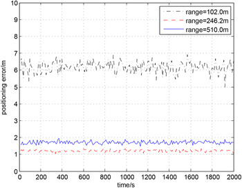
Figure 11. Relationship between the distance and the positioning error.
The simulation results indicate that the positioning accuracy depends directly on the PAM, and the optimal distance can apparently improve the positioning accuracy.
6. CONCLUSION
In this paper, we have investigated the problem of how to derive the optimal distance between the mobile buoy and the target to improve the positioning accuracy. The positioning model and error sources of MLBL have been developed. Considering the distance error and the position error of the mobile buoy, we propose the PAM to measure the positioning accuracy, based on which the optimal distance has been derived. We have shown that the optimal geometry is that the mobile buoys are on the vertices of the regular polygon centred at the target, and the optimal distance is related to the depth of the target and the parameter of the distance error. Simulation results have demonstrated the optimal distance and its effectiveness.
ACKNOWLEDGMENTS
This work was supported by the National Natural Science Foundation of China (NSFC) under grant 51209174, 61472325 and 61273333, the NSFC-RS joint research project under grants 51311130137 in China and IE121414 in UK, and the State Key Laboratory of Robotics and System (HIT) under grant SKLRS-2012-MS-04.


