2. Algorithm of constructing the exact solution

Let the fluid occupy a certain domain $D_{z0}$ in a physical plane $z = x + {\rm i} y$ at the initial time. The boundary of this domain is free, and its evolution in time is not known. Let us take an auxiliary complex plane $\zeta = \xi + {\rm i} \eta$. In this plane, we choose a certain simple canonical domain $D_\zeta$ (circle, half-plane or strip). One of the advantages of this approach is the fact that the flow region in the auxiliary plane $\zeta$ is fixed in time. The goal is to find the conformal mapping of the domain $D_\zeta$ to a variable domain $D_z$ occupied by the fluid in the plane $z$. This mapping is described by the formula $z = Z (\zeta, t)$, where $Z (\zeta, t)$ is an unknown function. Another sought function is the complex velocity $U (\zeta, t) = u - {\rm i} v$, where $(u, v)$ are the components of the fluid velocity vector $\boldsymbol {v}$.

The function $U$ is an analytical function. The validity of the Cauchy–Riemann conditions for this function follows from satisfying the conditions of potentiality and continuity of the flow of an ideal incompressible fluid:

(2.1)$$\begin{gather} \textrm{rot} \,\boldsymbol{v} = 0 \Rightarrow \frac{\partial u}{\partial y} = \frac{\partial v}{\partial x}, \end{gather}$$

(2.2)$$\begin{gather}\textrm{div} \,\boldsymbol{v} = 0 \Rightarrow \frac{\partial u}{\partial x} =- \frac{\partial v}{\partial y}. \end{gather}$$

Thus, finding the evolution of the fluid flow is reduced to finding two functions $U(\zeta, t)$ and $Z(\zeta, t)$ that are analytical in the domain $D_\zeta$ and satisfy the kinematic and dynamic conditions on the free boundary. These conditions are usually written in terms of a conformal mapping and a complex potential (see, e.g. Dyachenko et al. Reference Dyachenko, Dyachenko, Lushnikov and Zakharov2019). In our studies, we proposed to use a complex velocity instead of a complex potential. This was done for the first time by Karabut (Reference Karabut1991) and then discussed in more detail in Karabut, Petrov & Zhuravleva (Reference Karabut, Petrov and Zhuravleva2019). Let us consider derivation of these conditions in more detail.

The kinematic condition means that the free boundary is a fluid line, i.e. it consists of the same particles; hence, the projection of the velocity $\bar {U}$ of the fluid particle located on the free boundary and the projection of the velocity of the boundary itself $Z_t$ onto the normal to the free boundary coincide with each other. In other words, the vector $Z_t - \bar {U}$ is directed tangentially to the free boundary. Let us recall that the vector tangential to the free boundary is defined as $Z_s$ (therefore, the normal vector is $\textrm {i} Z_s$). Here, $s$ is the length of the arc corresponding to the free boundary in the plane $\zeta$. The scalar product of two vectors $Z_1$ and $Z_2$ is defined by the formula $\textrm {Re} [Z_1 \bar {Z}_2]$. Therefore, the kinematic condition can be written as

(2.3)\begin{equation} \textrm{Im}[Z_s(\bar{Z}_t - U)] = 0. \end{equation}

The dynamic condition means that the pressure on the free boundary is constant. In view of the Euler equation, this means that the acceleration vector is orthogonal to the free surface. To derive this condition, we denote the time by the letters $T$, $\tau$ and $t$, while the remaining independent variables are the Lagrangian coordinates, the Euler coordinates $x$, $y$ and the complex variable $\zeta$, respectively. In such a way, it is possible to avoid the confusion in writing partial derivatives with respect to time. Thus, though $T = \tau = t$, the partial derivatives with respect to these variables have different meanings and do not coincide, i.e.

(2.4)\begin{equation} \frac{\partial}{\partial T} \neq \frac{\partial}{\partial \tau} \neq \frac{\partial}{\partial t}. \end{equation}

As the acceleration is defined as $\bar {U}_T$, we obtain the dynamic condition

(2.5)\begin{equation} \textrm{Re} (Z_s U_T) = 0. \end{equation}

As $Z$ and $\tau$ are independent variables, then $Z_\tau = 0$, and

(2.6)\begin{equation} Z_\tau = Z_t + Z_\zeta \zeta_\tau = 0 \ \Rightarrow \ \zeta_\tau =- \frac{Z_t}{Z_\zeta}. \end{equation}

Therefore, we have

(2.7)\begin{equation} \frac{\partial}{\partial \tau} = \frac{\partial}{\partial t} - \frac{Z_t}{Z_\zeta} \frac{\partial}{\partial \zeta}. \end{equation}

Taking into account that

(2.8)\begin{equation} \frac{\partial}{\partial Z} = \frac{\partial \zeta}{\partial Z} \frac{\partial}{\partial \zeta}, \end{equation}

we obtain

(2.9)\begin{equation} \frac{\partial}{\partial T} = \frac{\partial}{\partial \tau} + \frac{\partial Z }{\partial T} \frac{\partial }{\partial Z} = \frac{\partial}{\partial \tau} + \bar{U} \frac{\partial }{\partial Z} = \frac{\partial}{\partial \tau} + \bar{U} \frac{\partial \zeta}{\partial Z} \frac{\partial}{\partial \zeta}, \end{equation}

and, hence,

(2.10)\begin{equation} \frac{\partial U}{\partial T} = \frac{\partial U}{\partial t} - \frac{Z_t}{Z_\zeta} \frac{\partial U}{\partial \zeta} + \bar{U} \frac{\partial \zeta}{\partial Z} \frac{\partial U}{\partial \zeta}. \end{equation}

Substituting the resultant expression (2.10) into condition (2.5) and noting that $U_\zeta \zeta _Z Z_s = U_s$, we can write the dynamic boundary condition as

(2.11)\begin{equation} \textrm{Re} (Z_s U_T) = \textrm{Re} (Z_s U_t - Z_t U_\zeta \zeta_Z Z_s + \bar{U} U_\zeta \zeta_Z Z_s) = \textrm{Re} (Z_s U_t - U_s (Z_t - \bar{U})) = 0. \end{equation}

Thus, the kinematic and dynamic boundary conditions take the form

(2.12)\begin{equation} \left.\begin{array}{c@{}} \textrm{Im} [Z_s (\bar{Z}_t - U)] = 0, \\ \textrm{Re} [Z_s U_t - U_s (Z_t - \bar{U})] = 0. \end{array}\right\} \end{equation}

Let us consider the special case of general boundary conditions (2.12). It should be noted that both boundary conditions (dynamic and kinematic conditions) are satisfied if the sought functions on the free boundary satisfy the following system of equations:

(2.13)\begin{equation} \left.\begin{array}{c@{}} Z_t = \bar{U}, \\ U_t = 0. \end{array}\right\} \end{equation}

Certainly, using the boundary conditions (2.13) instead of the dynamic and kinematic conditions (2.12), we reduce the set of solutions. However, (2.13) can be integrated, which allows finding exact solutions of the original problem. It follows from the second equation of system (2.13) that the function $U$ is independent of $t$; hence, $U (\zeta, t) = U(\zeta, 0) \equiv f(\zeta )$. Here $f(\zeta )$ is the initial complex velocity of the fluid. Integrating the first equation of system (2.13) on the free boundary, we obtain $Z(\zeta, t) = t \overline {f(\zeta )} + g(\zeta )$. Here $g(\zeta ) \equiv Z(\zeta, 0)$ is the initial conformal mapping.

Thus, the following relations are satisfied on the free boundary:

(2.14)\begin{equation} \left.\begin{array}{c@{}} U (\zeta, t) = f(\zeta), \\ Z(\zeta, t) = t \overline{f(\zeta)} + g(\zeta). \end{array}\right\} \end{equation}

As the left and right sides of the first equation of system (2.14) are analytical functions of the complex variable $\zeta$, which coincide on a certain line, then, by virtue of the analytical continuation principle, they coincide everywhere in the domain $D_\zeta$; therefore, we have found the function of the complex velocity $U (\zeta, t) = f(\zeta )$ everywhere in the domain. To continue the second equation, we need information about the domain shape and about the function $f(\zeta )$. Knowing the value of $\overline {f(\zeta )}$ on the free boundary, we have to find an analytical function $F(\zeta )$ that coincides with $\overline {f(\zeta )}$ on the free boundary. Then, by virtue of the analytical continuation principle, we can argue that the equation $Z(\zeta, t) = t F(\zeta ) + g(\zeta )$ is satisfied everywhere in the domain and coincides with the initial equation on the free boundary.

Thus, the following algorithm is proposed for finding exact solutions that describe the flow of an ideal fluid in the domain whose boundary is free.

1. 1. In the auxiliary plane $\zeta$, we choose a domain $D_\zeta$ corresponding to the domain occupied by the fluid in the plane $z$. In fact, this choice means setting the initial conformal mapping, i.e. the function $g(\zeta ) \equiv Z(\zeta, 0)$.

2. 2. We define the fluid velocity at the initial time. The initial complex velocity is taken to be an arbitrary analytical function or a function having pole-type singular points in the flow domain (these singular points can be interpreted as sources or sinks located in the flow domain). However, one has to understand that we can estimate whether the entire procedure of obtaining an exact solution for the chosen initial velocity was successful only after the last stage of the procedure (studying whether the resultant solution is analytical) is finalized. Knowing the form of the initial conformal mapping and the fluid velocity at $t =0$, we determine the function $f(\zeta ) \equiv U(\zeta, 0)$.

3. 3. Using the first equation of system (2.14), we find the explicit form of the complex velocity functions $U(\zeta, t)$ on the free boundary in the auxiliary plane $\zeta$. The principle of analytical continuation allows us to conclude that in this way we determined the complex velocity function everywhere in the domain where this function is analytical.

4. 4. We find the function $F(\zeta )$ coinciding with $\overline {f(\zeta )}$ on the free boundary and obtain a function performing the conformal mapping $Z(\zeta, t) = t F(\zeta ) + g(\zeta )$.

5. 5. We study singular points of the resultant functions. If the function of the conformal mapping is analytical in the flow domain, while the function of the complex velocity is analytical or has a pole-type singular point, we can conclude that the exact solution of the original problem was successfully derived.

For solutions found by this method, the acceleration $U_T$ is equal to zero on the free boundary. Indeed, it follows from (2.10) that

(2.15)\begin{equation} \frac{\partial U}{\partial T} = \frac{\partial U}{\partial t} - \frac{U_\zeta}{Z_\zeta} (Z_t - \bar{U}), \end{equation}

whence it follows in view of conditions (2.13) that the acceleration on the free boundary is ${\partial U}/{\partial T} = 0$.

3. Initial position of the fluid inside or outside the unit circle

Let us consider some examples of exact solutions obtained by the method described above. Let $g(\zeta ) = \zeta$. This means that $D_\zeta$ is chosen to be the domain occupied by the fluid at the initial time $D_{z0}$. One of the simplest cases is the exterior $|\zeta | > 1$ or the interior $|\zeta | < 1$ a unit circle. Let the initial complex velocity have a pole

(3.1)\begin{equation} U(z,0) = \frac{A}{z - \zeta_0} \quad (\textrm{Im}\,A = 0, \ \textrm{Im}\,\zeta_0 = 0). \end{equation}

Here, $A$ is the initial intensity of the source or sink, and $\zeta _0$ is a constant defining the source or sink position. Let us choose $\zeta _0$ in such a way that it is located in the domain $D_{z0}$. Thus, there is a source ($A > 0$) or a sink ($A < 0$) in the flow region at the initial time. Situations with the singularity $\zeta _0$ located inside the unit circle $|z| < 1$ or outside it $|z| > 1$ are principally different.

As the conformal mapping at $t = 0$ is performed by the function $Z(\zeta,0) = g(\zeta ) =\zeta$, the initial complex velocity in the plane $\zeta$ has the form

(3.2)\begin{equation} U(\zeta, 0) = f(\zeta) = \frac{A}{\zeta - \zeta_0}. \end{equation}

Knowing the function $f(\zeta )$, we determine the complex velocity for any value of $t$,

(3.3)\begin{equation} U(\zeta, t) = \frac{A}{\zeta - \zeta_0}. \end{equation}

Let us consider the second equation of system (2.14). Let us recall that it is satisfied on the free boundary corresponding to a unit circumference in the plane $\zeta$, i.e. $|\zeta | =1$, which means that $\zeta = \textrm {e}^{\textrm {i} \theta }$. In this case, we have

(3.4)\begin{equation} \bar{\zeta} = {\rm e}^{-{\rm i} \theta} = \frac{1}{\zeta}. \end{equation}

Thus, it follows from the second equation of system (2.14) that the function $Z(\zeta, t)$ on the free boundary $\zeta = \textrm {e}^{\textrm {i} \theta }$ has the form

(3.5)\begin{equation} Z (\zeta,t) = t \overline{f(\zeta)} + g(\zeta) = \zeta + \frac{A t}{1/\zeta - \zeta_0}, \quad \text{here } \zeta = {\rm e}^{{\rm i} \theta}. \end{equation}

Now it is possible to apply the analytical continuation principle to this function. Therefore, the problem is completely solved in the domain $D_\zeta$,

(3.6a,b)\begin{equation} U (\zeta, t) = \frac{A}{\zeta - \zeta_0}, \quad Z(\zeta, t) = \zeta + \frac{A t}{1/\zeta - \zeta_0}. \end{equation}

Eliminating the variable $\zeta$ from system (3.6), we obtain the form of the complex velocity in the physical plane $z$,

(3.7)\begin{equation} U(z,t) = \frac{A(A t + z \zeta_0 - 2 \zeta_0^2) \pm A \sqrt{(z \zeta_0 + A t -1)^2 + 4 A t}}{2(z(1-\zeta_0^2)-\zeta_0(A t + 1- \zeta_0^2))}. \end{equation}

Let us recall that the free boundary corresponds to the unit circumference $|\zeta | = 1$ in the plane $\zeta$. Assuming that $\zeta = \textrm {e}^{\textrm {i} \theta }$ in the second equation of system (3.6) and separating the real and imaginary parts, we obtain a parametric equation of the free boundary in the physical plane

(3.8a,b)\begin{equation} x = \textrm{Re} \left [{\rm e}^{{\rm i} \theta} + \frac{A t}{{\rm e}^{-{\rm i} \theta} - \zeta_0}\right], \quad y = \textrm{Im} \left [{\rm e}^{{\rm i} \theta} + \frac{A t}{{\rm e}^{-{\rm i} \theta} - \zeta_0}\right], \quad \text{here } \theta \in [0, 2{\rm \pi}]. \end{equation}

However, for the solution to describe a certain fluid flow adequately, its singular points should either be located outside the flow region or allow some hydrodynamic interpretation. Obviously, the function $U(\zeta, t)$ in the plane of the complex variable $\zeta$ has a pole at the point $\zeta _0$. Let us demonstrate that the corresponding point $z_0 = Z(\zeta _0,t)$ in the physical plane $z$ is also a pole of the complex velocity. For this purpose, we calculate the limit, which is equal to the source (sink) intensity in the physical plane,

(3.9)\begin{align} \lim_{z \rightarrow z_0} U ( z - z_0) &= \lim_{z \rightarrow z_0} \frac{A}{\zeta - \zeta_0} \left( \zeta -\zeta_0 + \frac{A t}{1/\zeta - \zeta_0} - \frac{A t}{1/\zeta_0 - \zeta_0}\right)\nonumber\\ & = A + \frac{A^2 t}{(1-\zeta^2_0)^2} \equiv B. \end{align}

It should be noted that the pole in the physical plane

(3.10)\begin{equation} z_0 = Z(\zeta_0,t) = \zeta_0 - \frac{A \zeta_0}{\zeta_0^2-1} t, \end{equation}

moves along the real axis with a constant velocity. This fact is difficult to explain from the physical point of view, but it is easily eliminated by transition to a new coordinate system moving relative to the initial one with constant velocity $u_0 = A \zeta _0/(\zeta _0^2-1)$. Indeed, let us use the Galilean transformation, denoting the new complex variable – $\tilde {z}$, the complex velocity in the new coordinate system – $\tilde {U}$. We denote the time in the new coordinate system by $\tilde {\tau }$. By virtue of the Galilean transformation, we have

(3.11)\begin{equation} \left.\begin{array}{c@{}} \tilde{\tau} = \tau, \\ \tilde{z} = z + u_0 \tau, \\ \tilde{U} = U + u_0. \end{array}\right\} \end{equation}

The pole position in the new system will be fixed,

(3.12)\begin{equation} \widetilde{z_0} = z_0 + u_0 \tau = \zeta_0 - \frac{A \zeta_0}{\zeta_0^2-1} + u_0 t = \zeta_0. \end{equation}

It is seen from presentation (3.7) that, in addition to the pole $z_0$, the function $U(z,t)$ has two more singular points of the square root type $z_1$ and $z_2$, which are the roots of the equation

(3.13)\begin{equation} (z \zeta_0 + A t -1)^2 + 4 A t =0. \end{equation}

If there is a sink at the singular point $z_0$, i.e. $A < 0$, then the singularities $z_1$ and $z_2$ move along the real axis $z_{1, 2} = (\sqrt {-A t} \pm 1)^2/\zeta _0$. In view of the free boundary equation (3.8), we can determine that one of the singularities in this case reaches the free boundary at the time instant $t^\ast = -(1- \zeta _0)^2/A$. Thus, the solution breaks down within a finite time due to the formation of the cusp point on the free boundary.

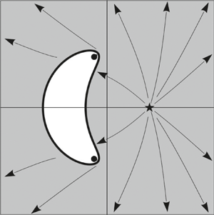
Figure 1 shows an example of such a flow. The domain occupied by the fluid is coloured grey, and the streamlines are shown there. At the initial time, the fluid occupies a unit circle. In the fluid region, at the point $z_0 = 1/2 - 2 t/3$, there is a singular point, which is a sink of intensity $A = -1$. This point is marked by the star in the figure. Two other singularities of the square root type have the form $z_{1, 2} = 2 (\sqrt {t} \pm 1)^2$. Arising at the initial time at the point $z =2$, they move along the real axis in the opposite directions (at $t < 1$). One of them passes to infinity and does not affect the solution. The other one, which is shown by the dot in the figure, approaches the free boundary and reaches it at $t^\ast = 1/4$, leading to solution breakdown. Thus, we obtain an example of the solution broken within a finite time due to the fact that the singular point initially located outside the flow region reaches the free boundary.

Figure 1. Evolution of a droplet with a sink.

Another situation is observed if there is a source in the fluid at the initial time, i.e. $A > 0$. In this case, it is more convenient to study the behaviour of singularities in the plane $\zeta$. Let us recall that the complex velocity function is not analytical at points where $Z_\zeta =0$ because $U_z = U_\zeta /Z_\zeta$. The second equation of system (3.6) yields

(3.14)\begin{align} Z_\zeta = 1 + \frac{A t (1- \zeta \zeta_0) + \zeta_0 A t \zeta}{(1- \zeta \zeta_0)^2} = 0 \ \Rightarrow \ (1- \zeta \zeta_0)^2 =- A t \ \Rightarrow \ \zeta = \frac{1}{\zeta_0} \pm {\rm i} \frac{\sqrt{A t}}{\zeta_0}. \end{align}

Therefore, there are two singularities in the plane $\zeta$ at $A > 0$, which are formed at the initial time on the real axis at the point $\xi = 1/\zeta _0$ and move along the straight line $\xi = 1/\zeta _0$ in the opposite directions to infinity. There may be two principally different cases here. In the first case, the fluid occupies a unit circle at the initial time and there is a source at a certain point $\zeta _0$ located on the real axis inside this circle ($|\zeta _0| < 1$); therefore, the singularities are always outside the fluid because the flow region is bounded by the unit circle and the singular points move along the straight line $\xi = 1/\zeta _0 > 1$. We obtain droplet spreading with a source, which is an example of the solution that exists for an unlimited time. Figure 2 illustrates the evolution of such a droplet at $A = 1$, $\zeta _0 = 1/2$. The domain occupied by the fluid is coloured grey, and the streamlines are shown. The source position is marked by the star.

Figure 2. Growth of the droplet containing a source.

The second case with the fluid initially occupying the exterior of the unit circle is much more interesting. There is a source in the flow region ($|\zeta _0| > 1$). We actually consider a bubble of a unit radius located in an unbounded fluid with a source. In this case, the singularities are formed inside the circle because $\xi = 1/\zeta _0 < 1$ and reach the free boundary $|\zeta | = 1$ at the time $t^\ast = (\zeta _0^2-1)/A$. The solution breaks down, and the bubble collapses. Let us study the shape of the free boundary in the plane $z$ at the instant of solution breakdown $t^\ast$. Substituting $t = t^\ast$ into the second equation of system (3.6), we find that the free boundary in the plane $z$ at the solution breakdown instant is defined by

(3.15)\begin{equation} \left. z = \zeta + \frac{A t \zeta}{1- \zeta \zeta_0} = \frac{\zeta \zeta_0 (\zeta_0 - \zeta)}{1- \zeta \zeta_0}\right|_{\zeta = {\rm e}^{{\rm i} \theta}}. \end{equation}

As $|\zeta |$ on the free boundary is equal to unity, we obtain that $|z|$ for the free boundary points has the form

(3.16)\begin{equation} |z| = |\zeta| |\zeta_0| \left|\frac{\zeta_0 - \zeta}{1- \zeta \zeta_0} \right| = |\zeta_0| \left|\frac{\zeta_0 - \zeta}{1- \zeta \zeta_0} \right|. \end{equation}

Let us calculate the absolute value assuming that $\zeta = \textrm {e}^{\textrm {i} \theta }$,

(3.17)\begin{equation} \left|\frac{\zeta_0 - \zeta}{1- \zeta \zeta_0} \right| = \left|\frac{\zeta_0 - \cos \theta - {\rm i} \sin \theta}{1- \zeta_0 \cos \theta - {\rm i} \zeta_0 \sin \theta} \right| = \left|\frac{(\zeta_0 - \cos \theta)^2 + \sin^2 \theta}{(1- \zeta_0 \cos \theta)^2 + \zeta_0^2 \sin^2 \theta} \right| = 1. \end{equation}

Substituting the absolute value (3.17) into (3.16), we find that the equality $|z| = |\zeta _0|$ is valid for the points located on the free boundary at the solution breakdown instant. Therefore, the free boundary at the bubble collapse instant transforms to an arc of a circumference of radius $|\zeta _0|$ with the centre at the origin of the coordinate system. Let us determine the degree measure of this arc. For this purpose, we study the smoothness of the free boundary in the plane $z$ at the time $t^\ast$. Let us recall that the equation of the free boundary in the physical plane can be derived as a parametrically defined curve. Assuming that $z = x + \textrm {i} y$ in (3.15) and separating the real and imaginary parts, we obtain

(3.18a,b)\begin{equation} x = \zeta_0 \left(\frac{2 \sin^2 \theta}{\zeta_0^2 - 2 \zeta_0 \cos \theta +1} -1\right), \quad y = \frac{2 \zeta_0 \sin \theta ( \zeta_0 - \cos \theta )}{\zeta_0^2 - 2 \zeta_0 \cos \theta +1}. \end{equation}

If the curve $y(x)$ is defined parametrically, then its smoothness is violated at those points where the derivative $x_\theta$ with respect to the parameter $\theta$ vanishes. After differentiating the first equation of system (3.18) with respect to $\theta$ and some transformations, we obtain

(3.19)\begin{equation} x_\theta = 0 \Leftrightarrow (\cos \theta - \zeta_0) (1 - \zeta_0 \cos \theta ) = 0. \end{equation}

In the case considered here, we have $|\zeta _0| > 1$; then it follows from (3.19) that $\theta = \pm \arccos (1/\zeta _0)$. For certainty, let us assume that $\zeta _0 = 2$. Substituting the found values of the parameters into (3.15), we see that the free boundary smoothness in this case is violated at the points $z = -1 \pm \textrm {i} \sqrt {3}$. It is of interest that the singularities $z_{1, 2}$, which reached the free boundary at the time $t^\ast$, are also located at the points $z = -1 \pm \textrm {i} \sqrt {3}$.

Figure 3 illustrates the evolution of the bubble located in an unbounded fluid. The domain occupied by the fluid is coloured grey, and the streamlines are shown. There is a source of intensity $A = 1$ in the fluid at the point $\zeta _0 = 2$ at the initial time. Its position is marked by the star. Two other singularities are formed at the initial time at the point $z = 1/2$. Then they separate from each other and move inside the bubble. Their positions are marked by the dots in the figure. At the time $t^\ast = 3$, the singularities reach the free boundary, and the bubble collapses into an arc of a circumference of radius $2$ (the value of this arc is $120^\circ$). The solution breaks down.

Figure 3. Evolution of the bubble located in an unbounded fluid with a source.

4. Initial form of the fluid is a strip

Let the fluid at the initial time occupy a strip

(4.1)\begin{equation} D_{z0} = \left\{(x, y) : - \infty < x <+\infty, \ -\frac{\rm \pi}{4} < y < \frac{\rm \pi}{4}\right\}, \end{equation}

bounded by free boundaries. We assume that a pole of the first order of intensity $A$ is located in the flow region at the origin and the velocity field at $t = 0$ is defined by the complex velocity of the form

(4.2)\begin{equation} U(z, 0) = \frac{A}{\tanh z}, \quad ({\rm Im}\,A = 0). \end{equation}

The flow domain in the auxiliary plane $D_\zeta$ is taken to be a unit circle with the centre at the origin of the coordinate system $\zeta = 0$. It is known that the strip $D_{z0}$ is mapped to a unit circle by the function $\zeta = \tanh z$; therefore, the function $g(\zeta ) \equiv Z(\zeta, 0)$ is taken to be an inverse function to the hyperbolic tangent

(4.3)\begin{equation} g(\zeta) = \tanh^{-1} z = \frac{1}{2} \ln \left(\frac{1+\zeta}{1-\zeta}\right). \end{equation}

The initial complex velocity in the plane $\zeta$ has the form $U(\zeta,0) = A/\zeta$. According to the solution algorithm described above, it follows that, for any $t$,

(4.4)\begin{equation} U(\zeta,t) = \frac{A}{\zeta}. \end{equation}

Let us find the function that performs conformal mapping. Let us recall that conditions (2.13) are satisfied on the free boundary corresponding to the unit circumference $|\zeta | = 1$ in the plane $\zeta$; therefore, the following transformations are valid for $\zeta = \textrm {e}^{\textrm {i} \theta }$ ($\theta \in [0, 2{\rm \pi} ]$):

(4.5)\begin{equation} Z_t = \bar{U} \ \Rightarrow \ Z_t = \overline{ \frac{A}{\zeta} } = A \zeta \Rightarrow \ Z = A \zeta t + g(\zeta). \end{equation}

This function is analytical; therefore, it may be continued from the free boundary to the entire plane $\zeta$. Thus, we obtain the problem solution in the auxiliary plane $\zeta$,

(4.6a,b)\begin{equation} U(\zeta,t) = \frac{A}{\zeta}, \quad Z(\zeta, t) = \frac{1}{2} \ln\left(\frac{1+\zeta}{1-\zeta}\right) + A \zeta t. \end{equation}

After the mapping defined by the second equation of system (4.6), the segment of the real axis $\xi \in [-1, 1]$ in the complex plane $\zeta$ is mapped into the abscissa axis in the plane $z$. The non-penetration condition is satisfied on this line, i.e.

(4.7)\begin{equation} U(\xi, t) = \frac{A}{\xi} = u - {\rm i} v \ \Rightarrow \ v \equiv 0. \end{equation}

Thus, it is possible to consider not only the flow in a strip bounded by two free boundaries, which was initially declared, but it is also possible to talk about the flow of a fluid layer on a motionless solid wall.

Let us study the singular points of the constructed solution. In the auxiliary plane $\zeta$, the complex velocity has a pole at the point $\zeta = 0$. This point corresponds to $z =0$ in the physical plane. Let us calculate the limit $\lim _{z \rightarrow 0} (z U)$ and show that there is also a pole in the plane $z$ at the origin of the coordinate system:

(4.8)\begin{align} \lim_{z \rightarrow 0} z U& = \lim_{\zeta \rightarrow 0} \left(\frac{A}{2 \zeta} \ln \frac{1+\zeta}{1-\zeta} + A^2 t \right)\nonumber\\ & = \lim_{\zeta \rightarrow 0} \left( \frac{A}{2 \zeta} \ln \left( 1 + \frac{2 \zeta}{1-\zeta}\right) + A^2 t \right) = A + A^2 t. \end{align}

Thus, the complex velocity function in the physical plane has a source or a sink of variable intensity linearly increasing with time at the origin of the coordinate system.

In addition to the pole, the analytical character of the complex velocity function is violated at the points $Z_\zeta = 0$. Let us study these points in the plane $\zeta$,

(4.9)\begin{equation} Z_\zeta = \frac{\partial}{\partial \zeta}\left(\frac{1}{2} \ln\left(\frac{1+\zeta}{1-\zeta}\right) + A \zeta t \right) = \frac{1}{1-\zeta^2} + A t = 0 \ \Rightarrow \ \zeta^2 = 1+\frac{1}{A t}. \end{equation}

If the fluid at the initial time contains a source $(A > 0)$, then the singularities defined by (4.9) arise at infinitely distant points and move along the real axis. However, these singular points reach the boundaries of the flow region $|\zeta |<1$ only as $t \rightarrow \infty$ because

(4.10)\begin{equation} \lim_{t \rightarrow \infty} \left( 1+\frac{1}{A t} \right) = 1. \end{equation}

Therefore, there is only one singularity (source) inside the flow region at any finite time instant. Thus, we constructed an example of the exact solution that describes the fluid flow with a free boundary located on a motionless solid surface with a source. As a result, a droplet growing with time is formed on the free surface. This process is illustrated in figure 4. The domain occupied by the fluid is coloured grey, and the streamlines are shown. The source marked by the star is located at the origin of the coordinate system. Two singularities (marked by the dots in the figure) move outside the flow region, form the line of the free boundary and approach it as $t \rightarrow \infty$.

Figure 4. Fluid flow on a solid substrate containing a source.

If there is a sink $(A < 0)$ at the initial time on the solid wall bounding the flow region, the singular points defined by (4.9) move at $t \in (0, -1/A)$ along the imaginary axis toward each other from infinity to the origin:

(4.11)\begin{equation} \zeta^\ast= \pm {\rm i} \sqrt{- 1 - 1/(A t)}. \end{equation}

Obviously, they will cross the free boundary $|\zeta | = 1$ at a certain time instant and enter the flow region. The instant of solution breakdown is easily calculated, i.e.

(4.12)\begin{equation} \zeta^\ast= {\rm i} \sqrt{- 1 - 1/(A t^\star)} = {\rm i} \ \Rightarrow \ \sqrt{- 1 - 1/(A t^\star)} = 1 \ \Rightarrow \ t^\star=- \frac{1}{2 A}. \end{equation}

Thus, we constructed an example of the solution that describes the fluid flow with a free boundary on a solid substrate with a sink. The solution breaks down within a finite time with the formation of a cusp point on the free boundary. The evolution of such a flow at $A = -1$ is illustrated in figure 5. The domain occupied by the fluid is coloured grey, and the streamlines are shown. The sink located at the origin of the coordinate system is marked by the star. Two other singularities, as was shown above, move along the imaginary axis. One of them, which has a negative coordinate, does not affect the flow at all. The other one, which is marked by the dot in the figure, approaches the free boundary and forms a dip on it. At the time $t^\star = 1/2$, the singular point reaches the flow region boundary, thus breaking the solution.

Figure 5. Fluid flow on a solid substrate containing a sink.

5. Method of conformal mappings and Hopf equation

In our previous publications (Karabut & Zhuravleva Reference Karabut and Zhuravleva2014; Karabut et al. Reference Karabut, Zhuravleva and Zubarev2020), we found exact solutions that describe flows with zero acceleration on the free boundary by using the Hopf equation $U_\tau + U U_z =0$ or its generalization in the form

(5.1)\begin{equation} U_\tau + C(U) U_z = 0, \end{equation}

where $C(U)$ is a rational function depending on the complex velocity. Solutions were found for the cases with $C(U) = U$, $C(U) = -U$ and $C(U) = 1/U$. It is of interest to note that the solutions found in the present study also satisfy the generalized Hopf equation (5.1). Let us demonstrate this fact. According to (2.7), we have

(5.2)\begin{equation} U_\tau = U_t -\frac{Z_t}{Z_\zeta} U_\zeta. \end{equation}

Let us recall that we tried to find solutions satisfying system (2.13); hence, $U_t =0$ for them. Then, taking into account that $U_\zeta /Z_\zeta = U_z$, we can rewrite (5.2) in the form

(5.3)\begin{equation} U_\tau =- Z_t U_z \ \Rightarrow \ U_\tau + Z_t U_z = 0. \end{equation}

Comparing (5.1) and (5.3), we see that the solutions obtained in the present study satisfy the generalized Hopf equation with the function $C(U) = Z_t$.

Let us find the explicit form of the function $C(U)$ for solutions where the free boundary in the physical plane at the initial time is a unit circumference. According to the second equation of system (3.6), we have

(5.4)\begin{equation} Z(\zeta, t) = \zeta + \frac{A t}{1/\zeta -\zeta_0} \ \Rightarrow \ Z_t = \frac{A}{1/\zeta -\zeta_0}. \end{equation}

From the first equation of system (3.6), we express $\zeta$ via $U$ and substitute it into the expression for $Z_t$, thus obtaining

(5.5)\begin{equation} U(\zeta, t) = \frac{A}{\zeta - \zeta_0}\ \Rightarrow\ \zeta = \frac{A}{U} + \zeta_0 \Rightarrow \ Z_t = \frac{A}{\dfrac{U}{A + U \zeta_0} -\zeta_0} = \frac{A^2+ A U \zeta_0}{(1-\zeta_0^2) U - A \zeta_0}. \end{equation}

Therefore, the solutions found in the present study for which the free boundary at the initial time is a unit circle satisfy the generalized Hopf equation (5.1) with the function $C(U)$ of the form

(5.6)\begin{equation} C(U) = \frac{A^2 + A U \zeta_0}{(1-\zeta_0^2) U - A \zeta_0}. \end{equation}

Thus, we extended the family of the functions $C(U)$ for which the solutions of the generalized Hopf equation describe the ideal fluid flow with a free boundary. However, if we apply the Galileo transformation (3.11) and pass to the coordinate system with respect to which the pole of the complex velocity is stationary, it turns out that the found flows are described by the generalized Hopf equation for which

(5.7)\begin{equation} C(\tilde{U}) = \frac{A^2}{(1-\zeta_0^2)^2 \tilde{U}}. \end{equation}