


1 Introduction
1.1 The description of our result
The quantum toroidal algebra $U_{q_1,q_2}(\ddot {gl}_1)$
(Definition 1.3) is an affinisation of the quantum Heisenberg algebra which has been realised in several contexts:
$U_{q_1,q_2}(\ddot {gl}_1)$
(Definition 1.3) is an affinisation of the quantum Heisenberg algebra which has been realised in several contexts:
-
• the elliptic Hall algebra in [Reference Burban and Schiffmann2, Reference Schiffmann30],
-
• the double shuffle algebra in [Reference Feigin, Hashizume, Hoshino, Shiraishi and Yanagida8, Reference Feigin and Odesskii9, Reference Neguţ23],
-
• the trace of the deformed Khovanov Heisenberg category in [Reference Cautis, Lauda, Licata, Samuelson and Sussan4](when $q_1=q_2$
).
$q_1=q_2$
).

Given a smooth quasiprojective surface S over $k=\mathbb {C}$
, let
$k=\mathbb {C}$
, let
 $$ \begin{align*}\mathcal{M}=\bigsqcup_{n=0}^{\infty} S^{[n]}\end{align*} $$
be the Hilbert schemes of points on S. Schiffmann-Vasserot [Reference Schiffmann and Vasserot32], Feigin-Tsymbaliuk [Reference Feigin and Tsymbaliuk10] and Neguţ [Reference Neguţ26] constructed the $U_{q_1,q_2}(\ddot {gl}_1)$
action on the Grothendieck group of
$U_{q_1,q_2}(\ddot {gl}_1)$
action on the Grothendieck group of $\mathcal {M}$
. It generalises the action of
$\mathcal {M}$
. It generalises the action of
-
• the Heisenberg algebra (Nakajima [Reference Nakajima22] and Grojnowski [Reference Grojnowski11])
-
• the W algebra (Li-Qin-Wang [Reference Li, Qin and Wang21])
on the cohomology of Hilbert schemes.
The main result of this paper is a weak categorification of the above quantum toroidal algebra action. First let us state our results precisely. Given a nonnegative integer n, let $S^{[n,n+1]}$
be the nested Hilbert scheme
$S^{[n,n+1]}$
be the nested Hilbert scheme
 $$ \begin{align*}S^{[n,n+1]}:=\{(\mathcal{I}_n,\mathcal{I}_{n+1},x)\in S^{[n]}\times S^{[n+1]}\times S|\mathcal{I}_{n+1}\subset \mathcal{I}_n, \mathcal{I}_n/\mathcal{I}_{n+1}=k_x\},\end{align*} $$
which is a closed subscheme of $S^{[n]}\times S^{[n+1]}\times S$
. There is a tautological line bundle
$S^{[n]}\times S^{[n+1]}\times S$
. There is a tautological line bundle ${\mathcal {L}}$
on
${\mathcal {L}}$
on $S^{[n,n+1]}$
, such that its fibre at each closed point is
$S^{[n,n+1]}$
, such that its fibre at each closed point is $\mathcal {I}_{n}/\mathcal {I}_{n+1}$
. We abuse the notation to denote
$\mathcal {I}_{n}/\mathcal {I}_{n+1}$
. We abuse the notation to denote $\mathcal {I}$
as the universal ideal sheaf on
$\mathcal {I}$
as the universal ideal sheaf on ${\mathcal {M}}{\times }S$
. We will write
${\mathcal {M}}{\times }S$
. We will write $S_1,S_2$
for two copies of S, in order to emphasise the factors of
$S_1,S_2$
for two copies of S, in order to emphasise the factors of $S\times S$
. Let
$S\times S$
. Let ${\Delta }:{\mathcal {M}}{\times }S{\to }{\mathcal {M}}{\times }{\mathcal {M}}{\times }S_{1}{\times }S_{2}$
be the diagonal embedding and
${\Delta }:{\mathcal {M}}{\times }S{\to }{\mathcal {M}}{\times }{\mathcal {M}}{\times }S_{1}{\times }S_{2}$
be the diagonal embedding and $\iota :{\mathcal {M}}{\times }{\mathcal {M}}{\times }S_{1}{\times }S_{2}{\to }{\mathcal {M}}{\times }{\mathcal {M}}{\times }S_{2}{\times }S_{1}$
be the involution map which changes the order of two copies of S. We denote
$\iota :{\mathcal {M}}{\times }{\mathcal {M}}{\times }S_{1}{\times }S_{2}{\to }{\mathcal {M}}{\times }{\mathcal {M}}{\times }S_{2}{\times }S_{1}$
be the involution map which changes the order of two copies of S. We denote $D^{b}(X)$
to be the (bounded) derived categories of coherent sheaves on a given scheme X. We prove that
$D^{b}(X)$
to be the (bounded) derived categories of coherent sheaves on a given scheme X. We prove that
Theorem 1.1 (Theorem 5.1, see Section 1.8 for the notations).
Consider the Fourier-Mukai kernels $e_k,f_k:D^b(\mathcal {M})\to D^b(\mathcal {M}\times S)$
induced from:
$e_k,f_k:D^b(\mathcal {M})\to D^b(\mathcal {M}\times S)$
induced from:
 $$ \begin{align*} e_{k}:=\mathcal{L}^{k}\mathcal{O}_{S^{[n,n+1]}}\in D^b(S^{[n]}\times S^{[n+1]}\times S) \\ f_k:=\mathcal{L}^{k-1}\mathcal{O}_{S^{[n,n+1]}}[1]\in D^b(S^{[n+1]}\times S^{[n]}\times S). \end{align*} $$
-
(1) For every two integers m and r, there exists natural transformations
(1.1)
$$ \begin{align} \begin{cases} f_re_{m-r}\to \iota_{*}e_{m-r}f_r & \text{ if } m>0 \\ \iota_{*}e_{m-r}f_r\to f_re_{m-r} & \text{ if } m<0 \\ f_re_{-r}=\iota_{*}e_rf_{-r}\oplus \mathcal{O}_{\Delta}[1] \end{cases} ,\end{align} $$
where
$\Delta $
is the diagonal of
$\mathcal {M}\times \mathcal {M}\times S \times S$
. -
(2) When
$m\neq 0$
, the cone of the natural transformations in (1.1) has a filtration with associated graded object
$$ \begin{align*} \begin{cases} \bigoplus\limits_{k=0}^{m-1}R\Delta_*(h_{m,k}^{+}) & \text{ if } m>0 \\ \bigoplus\limits_{k=m+1}^{0}R\Delta_*(h_{m,k}^{-}) & \text{ if } m<0 \end{cases} ,\end{align*} $$
where
$h_{m,k}^{+},h_{m,k}^{-}\in D^{b}(\mathcal {M}\times S)$
are complexes of wedge and symmetric product of universal sheaves on
$\mathcal {M}\times S$
.


It is natural to expect that Theorem 1.1 should be compatible with the computation in [Reference Neguţ24], which we show in Theorem 3.2.
The nontriviality of the extension is a feature of the derived category statement, which is not visible at the level of Grothendieck groups. Proposition 6.3 provides a precise extension formula.
1.2 The weak categorification of an algebra action
Categorification can take place in a very general setting. Roughly speaking, it lifts a certain quantity to a chain complex whose Betti number is the quantity. Here we follow the notation of Savage [Reference Savage29] for the naive, weak and strong categorifications of algebra and representations.
Let A be a commutative ring and $B=(\{b_{i}\}_{i,\in I},\{c_{j}\}_{j\in J})$
be a unitial associative A-algebra, where
$B=(\{b_{i}\}_{i,\in I},\{c_{j}\}_{j\in J})$
be a unitial associative A-algebra, where $\{b_{i}\}_{i\in I}$
is the generating set and
$\{b_{i}\}_{i\in I}$
is the generating set and $\{c_{j}\}_{j\in J}$
is a set of relations which generate all the relations in B. Let M be a B-module. The action of each
$\{c_{j}\}_{j\in J}$
is a set of relations which generate all the relations in B. Let M be a B-module. The action of each $b_{i}$
defines an endomorphism
$b_{i}$
defines an endomorphism $b_{i}^{M}$
of M and each
$b_{i}^{M}$
of M and each $c_{j}$
defines a relation in the endomorphism ring of M which we denote as
$c_{j}$
defines a relation in the endomorphism ring of M which we denote as $c_{j}^{M}$
. For a triangulated category
$c_{j}^{M}$
. For a triangulated category $\mathcal {M}$
, we denote
$\mathcal {M}$
, we denote $K_{0}({\mathcal {M}})$
as the Grothendieck group of
$K_{0}({\mathcal {M}})$
as the Grothendieck group of ${\mathcal {M}}$
. For any
${\mathcal {M}}$
. For any $F\in {\mathcal {M}}$
, we denote
$F\in {\mathcal {M}}$
, we denote $[F]\in K_{0}({\mathcal {M}})$
as the class generated by F.
$[F]\in K_{0}({\mathcal {M}})$
as the class generated by F.
Definition 1.2 (Weak categorification).
A weak categorification of $(B,\{b_{i}\},\{c_{i}\},M)$
is a quadruple
$(B,\{b_{i}\},\{c_{i}\},M)$
is a quadruple $({\mathcal {M}},\phi ,\{F_{i}\}_{i\in I},\{E_{i}\}_{j\in J})$
, where
$({\mathcal {M}},\phi ,\{F_{i}\}_{i\in I},\{E_{i}\}_{j\in J})$
, where
-
(1)
${\mathcal {M}}$
is a triangulated category with an isomorphism
$\phi :K_{0}({\mathcal {M}})\to M$
; -
(2) for each
$i\in I$
,
$F_{i}:{\mathcal {M}}\to {\mathcal {M}}$
is an triangulated endofunctor of
${\mathcal {M}}$
, such that
$[F_{i}]=b_{i}^{M}$
under the isomorphism
$\phi $
; -
(3) for each
$j\in J$
,
$E_{j}=\{E_{j}^{1}\xrightarrow {e_{j}^{1}}E_{j}^{2}\xrightarrow {e_{j}^{2}}E_{j}^{3}\}$
, where
$E_{j}^{1},E_{j}^{2},E_{j}^{3}$
are endofunctors of
${\mathcal {M}}$
which are generated by
$F_{i}$
,
$e_{j}^{1}$
and
$e_{j}^{2}$
are natural transformations, such that for each element
$K\in {\mathcal {M}}$
,
$E_{j}^{1}(K)\xrightarrow {e_{j}^{1}(K)}E_{j}^{2}(K)\xrightarrow {e_{j}^{3}(K)}E_{j}^{3}(K)$
is an exact triangle in
${\mathcal {M}}$
and the relation
$c_{j}^{M}=\{[E_{j}^{1}]-[E_{j}^{2}]+[E_{j}^{3}]=0\}$
under the isomorphism
$\phi $
.


Now we recall an integral version of the quantum toroidal algebra $U_{q_1,q_2}(\ddot {gl}_1)$
.
$U_{q_1,q_2}(\ddot {gl}_1)$
.
Definition 1.3 ([Reference Neguţ26]).
Given two formal parameters $q_1$
and
$q_1$
and $q_2$
, let
$q_2$
, let $q=q_1q_2$
. Let
$q=q_1q_2$
. Let $\mathbb {K}=\mathbb {Z}[q_1+q_{2},q,q^{-1}]$
. The quantum toroidal algebra
$\mathbb {K}=\mathbb {Z}[q_1+q_{2},q,q^{-1}]$
. The quantum toroidal algebra $U_{q_1,q_2}(\ddot {gl_1})$
is the
$U_{q_1,q_2}(\ddot {gl_1})$
is the $\mathbb {K}$
-algebra with generators:
$\mathbb {K}$
-algebra with generators:
 $$ \begin{align*} \{E_{k},F_{k},H_{l}^{\pm}\}_{k\in \mathbb{Z},l\in \mathbb{N}} \end{align*} $$
modulo the following relations:
 $$ \begin{align} (z-wq_1)(z-wq_2)(z-\frac{w}{q})E(z)&E(w)= \\ &\quad =(z-\frac{w}{q_1})(z-\frac{w}{q_2})(z-wq)E(w)E(z) \notag \end{align} $$
 $$ \begin{align} (z-wq_1)(z-wq_2)(z-\frac{w}{q})E(z)&H^{\pm}(w)= \\ & \ \ =(z-\frac{w}{q_1})(z-\frac{w}{q_2})(z-wq)H^{\pm}(w)E(z) \notag \end{align} $$
 $$ \begin{align} [[E_{k+1},E_{k-1}],E_k]=0 \quad \forall k\in \mathbb{Z} \end{align} $$
together with the opposite relations for $F(z)$
instead of
$F(z)$
instead of $E(z)$
, as well as:
$E(z)$
, as well as:
 $$ \begin{align} [E(z),F(w)]=\delta(\frac{z}{w})(1-q_1)(1-q_2)(\frac{H^+(z)-H^{-}(w)}{1-q}) ,\end{align} $$
where
 $$ \begin{align} E(z)=\sum_{k\in \mathbb{Z}}\frac{E_k}{z^k}, \quad F(z)=\sum_{k\in \mathbb{Z}}\frac{F_k}{z^k}, \quad H^{\pm}(z)=\sum_{l\in \mathbb{N}\cup \{0\}}\frac{H_l^{\pm}}{z^{\pm l}} ,\end{align} $$
where
 $$ \begin{align*} \delta(z)=\sum_{n\in \mathbb{Z}}z^n\in \mathbb{Q}\{\{z\}\}. \end{align*} $$
We will set $H_0^+=q$
and
$H_0^+=q$
and $H_0^{-}=1$
.
$H_0^{-}=1$
.
The weak categorification of relations (1.2), (1.3), (1.4) was obtained in the main theorem of [Reference Neguţ26]. Hence, we still need to categorify (1.5) to obtain a weak categorification of the quantum toroidal algebra action, which is the purpose of Theorem 1.1.
1.3 Outline of the proof
Let us first review the categorification of the commutation of $e_k$
and
$e_k$
and $e_l$
for different k and l in [Reference Neguţ26]. Consider the moduli spaces
$e_l$
for different k and l in [Reference Neguţ26]. Consider the moduli spaces $\mathfrak {Z}_2,\mathfrak {Z}_{2}'$
which parameterise diagrams
$\mathfrak {Z}_2,\mathfrak {Z}_{2}'$
which parameterise diagrams
respectively, of ideal sheaves, where each successive inclusion is colength $1$
and supported at the point indicated on the diagrams. Then
$1$
and supported at the point indicated on the diagrams. Then $e_ke_l$
and
$e_ke_l$
and $e_le_k$
are the derived pushfoward of line bundles on
$e_le_k$
are the derived pushfoward of line bundles on $\mathfrak {Z}_2$
and
$\mathfrak {Z}_2$
and $\mathfrak {Z}_2'$
to
$\mathfrak {Z}_2'$
to $S^{[n-1]}\times S^{[n+1]}\times S\times S$
, respectively. In order to compare
$S^{[n-1]}\times S^{[n+1]}\times S\times S$
, respectively. In order to compare $e_ke_l$
and
$e_ke_l$
and $e_le_k$
, [Reference Neguţ26] introduced the quadruple moduli space
$e_le_k$
, [Reference Neguţ26] introduced the quadruple moduli space $\mathfrak {Y}$
which parameterises the diagram
$\mathfrak {Y}$
which parameterises the diagram

of ideal sheaves, where each successive inclusion is colength $1$
and supported at the point indicated on the diagrams.
$1$
and supported at the point indicated on the diagrams. $\mathfrak {Y}$
is smooth and induces resolutions of
$\mathfrak {Y}$
is smooth and induces resolutions of $\mathfrak {Z}_{2}$
and
$\mathfrak {Z}_{2}$
and $\mathfrak {Z}_{2}'$
. Proposition 2.30 of [Reference Neguţ26] proved that
$\mathfrak {Z}_{2}'$
. Proposition 2.30 of [Reference Neguţ26] proved that $\mathfrak {Z}_{2}$
and
$\mathfrak {Z}_{2}$
and $\mathfrak {Z}_{2}'$
are rational singularities, based on the fact that any fibre of the resolution has dimension
$\mathfrak {Z}_{2}'$
are rational singularities, based on the fact that any fibre of the resolution has dimension $\leq 1$
. Thus,
$\leq 1$
. Thus, $e_ke_l$
and
$e_ke_l$
and $e_le_k$
could be compared through line bundles on
$e_le_k$
could be compared through line bundles on $\mathfrak {Y}$
.
$\mathfrak {Y}$
.
Now in order to compare $f_re_{m-r}$
and
$f_re_{m-r}$
and $e_{m-r}f_r$
, we introduce the triple moduli spaces
$e_{m-r}f_r$
, we introduce the triple moduli spaces $\mathfrak {Z}_+,\mathfrak {Z}_{-}$
which parameterise diagrams
$\mathfrak {Z}_+,\mathfrak {Z}_{-}$
which parameterise diagrams


Then $f_re_{m-r}$
and
$f_re_{m-r}$
and $e_{m-r}f_r$
are the derived pushforward of line bundles on
$e_{m-r}f_r$
are the derived pushforward of line bundles on $\mathfrak {Z}_+,\mathfrak {Z}_{-}$
, respectively. The quadruple moduli space
$\mathfrak {Z}_+,\mathfrak {Z}_{-}$
, respectively. The quadruple moduli space $\mathfrak {Y}$
still induces resolutions of
$\mathfrak {Y}$
still induces resolutions of $\mathfrak {Z}_{-}$
, but
$\mathfrak {Z}_{-}$
, but $\mathfrak {Z}_{+}$
have two irreducible components. One irreducible component is
$\mathfrak {Z}_{+}$
have two irreducible components. One irreducible component is $S^{[n,n+1]}$
, denoted by
$S^{[n,n+1]}$
, denoted by $W_1$
, and the other irreducible component is denoted by
$W_1$
, and the other irreducible component is denoted by $W_0$
in Section 6.
$W_0$
in Section 6. $\mathfrak {Y}$
induces a resolution of
$\mathfrak {Y}$
induces a resolution of $W_0$
.
$W_0$
.
In order to compare $f_re_{m-r}$
and
$f_re_{m-r}$
and $e_{m-r}f_r$
through line bundles on
$e_{m-r}f_r$
through line bundles on $\mathfrak {Y}$
, one must prove that
$\mathfrak {Y}$
, one must prove that $\mathfrak {Z}_{-}$
and
$\mathfrak {Z}_{-}$
and $W_0$
are rational singularities. The approach in [Reference Neguţ26] did not work here, as the fibre could have pretty large dimensions. Instead, we study the singularity structure of
$W_0$
are rational singularities. The approach in [Reference Neguţ26] did not work here, as the fibre could have pretty large dimensions. Instead, we study the singularity structure of $\mathfrak {Z}_{+}$
and
$\mathfrak {Z}_{+}$
and $\mathfrak {Z}_-$
through the viewpoint of the minimal model program (MMP) [Reference Kollár17, Reference Kollár and Mori18]. We prove that
$\mathfrak {Z}_-$
through the viewpoint of the minimal model program (MMP) [Reference Kollár17, Reference Kollár and Mori18]. We prove that
Proposition 1.4 (Propositions 4.6 and 4.13).
The pair $(\mathfrak {Z}_+,0)$
is semi-dlt.
$(\mathfrak {Z}_+,0)$
is semi-dlt. $\mathcal {Z}_{-}$
and
$\mathcal {Z}_{-}$
and $W_0$
are canonical singularities.
$W_0$
are canonical singularities.
We prove Proposition 1.4 by explicitly computing the discrepancy (see Section 6 for the definitions of semi-dlt, canonical singularities and the discrepancy). Canonical singularities are always rational singularities by Theorem B.7.
Remark 1.5. One should notice the elliptic Hall algebra of [Reference Burban and Schiffmann2] contains more relations than Definition 1.3, which we would investigate in the future. The main obstacle of generalising our result to the elliptic Hall algebra is that for the action of other operators, the corresponding nested moduli space is not Cohen-Macaulay, and, hence, the enhancement in derived algebraic geometry has to be considered. It is also the obstacle of generalising our result to the quantum toroidal algebra action on the Grothendieck group of higher rank stable sheaves [Reference Neguţ26], as $\mathfrak {Z}_+$
is no longer equidimensional in this situation.
$\mathfrak {Z}_+$
is no longer equidimensional in this situation.
1.4 Categorical Heisenberg actions
Khovanov [Reference Khovanov16] defined the Heisenberg category through graphical calculus. Cautis-Licata [Reference Cautis and Licata5] constructed a categorical Heisenberg action on the derived category of Hilbert schemes of points of the minimal resolution of the type ADE singularities. Krug [Reference Krug20] constructed the weak categorical Heisenberg action on the derived category of Hilbert schemes of points on smooth surfaces. Our categorification is different from those above, as it is given in terms of explicit correspondences and independent of the derived McKay correspondence.
Although the higher Nakajima operators were categorified by the objects $e_{(0,\ldots ,0)}$
of [Reference Neguţ26], the relations between them (as well as the morphisms between them in Khovanov’s Heisenberg category) are still unclear to us.
$e_{(0,\ldots ,0)}$
of [Reference Neguţ26], the relations between them (as well as the morphisms between them in Khovanov’s Heisenberg category) are still unclear to us.
1.5 Double categorified Hall algebra
The study of Cohomological Hall algebra was initiated by Kontsevich-Soibelman [Reference Kontsevich and Soibelman19] and Schiffmann-Vasserot [Reference Schiffmann and Vasserot31]. Kapranov-Vasserot [Reference Kapranov and Vasserot15] and the author [Reference Zhao37] constructed the K-theoretic Hall algebra on surfaces, which was categorified by Porta-Sala [Reference Porta and Sala27]. It also categorified the positive half of $U_{q}(\ddot {gl}_1)$
when
$U_{q}(\ddot {gl}_1)$
when $S=\mathbb {A}^2$
. The relation between the categorified Hall algebra of minimal resolution of type A singularities and quivers was studied by Diaconescu-Porta-Sala [Reference Diaconescu, Porta and Sala6]. On the other hand, the Drinfeld double of the categorified Hall algebra is still mysterious. As an attempt to understand the action of the ‘double Categorified Hall algebra’, it is natural to expect that our approach could be generalised to categorifications in other settings, like those of Toda [Reference Toda36] and Rapcak-Soibelman-Yang-Zhao [Reference Rapcak, Soibelman, Yang and Zhao28].
$S=\mathbb {A}^2$
. The relation between the categorified Hall algebra of minimal resolution of type A singularities and quivers was studied by Diaconescu-Porta-Sala [Reference Diaconescu, Porta and Sala6]. On the other hand, the Drinfeld double of the categorified Hall algebra is still mysterious. As an attempt to understand the action of the ‘double Categorified Hall algebra’, it is natural to expect that our approach could be generalised to categorifications in other settings, like those of Toda [Reference Toda36] and Rapcak-Soibelman-Yang-Zhao [Reference Rapcak, Soibelman, Yang and Zhao28].
1.6 Other related work
Recently, Addington-Takahashi [Reference Takahashi35] studied certain sequences of moduli spaces of sheaves on $K3$
surfaces and showed that these sequences can be given the structure of a geometric categorical
$K3$
surfaces and showed that these sequences can be given the structure of a geometric categorical $\mathfrak {sl}_2$
action in the sense of [Reference Cautis, Kamnitzer and Licata3]. It would be interesting to explore the interactions between their action and ours.
$\mathfrak {sl}_2$
action in the sense of [Reference Cautis, Kamnitzer and Licata3]. It would be interesting to explore the interactions between their action and ours.
Another related work is Jiang-Leung’s projectivisation formula [Reference Jiang and Leung14]. Through this formula, they obtained a semiorthogonal decomposition of the derived category of the nested Hilbert schemes.
1.7 The organisation of the paper
The proof of the main theorem is in Section 5 and the extension formula is in Section 6. The other sections are organised as follows:
-
Section 2: we review the action of
$U_{q_1,q_2}(\ddot {gl}_1)$
on the Grothendieck group of Hilbert schemes [Reference Feigin and Tsymbaliuk10, Reference Neguţ24, Reference Neguţ26, Reference Schiffmann and Vasserot32]; -
Section 3: we define
$h_{m,k}^{+}\in D^b(\mathcal {M}\times S)$
and prove the third part of Theorem 1.1; -
Section 4: we study the singularity structures of
$\mathfrak {Z}_{-}$
and
$\mathfrak {Z}_{+}$
through the singularity theory of the minimal model program.


1.8 Notations
In this paper, we will always work over $k=\mathbb {C}$
.
$k=\mathbb {C}$
.
1.8.1 Derived categories and the Grothendieck groups
For any scheme X, we denote $D_{qcoh}(X)$
as the derived category of quasicoherent sheaves on X. We denote
$D_{qcoh}(X)$
as the derived category of quasicoherent sheaves on X. We denote $D^{u}(X)$
as the full subcategory of
$D^{u}(X)$
as the full subcategory of $D_{qcoh}(X)$
which consists of elements, such that all the cohomologies are coherent sheaves on X. We denote
$D_{qcoh}(X)$
which consists of elements, such that all the cohomologies are coherent sheaves on X. We denote $D^{b}(X)$
as the full subcategory of
$D^{b}(X)$
as the full subcategory of $D^{u}(X)$
, such that the cohomologies are bounded. We denote
$D^{u}(X)$
, such that the cohomologies are bounded. We denote $K(X):=K_{0}(D^{b}(X))$
.
$K(X):=K_{0}(D^{b}(X))$
.
1.8.2 Fourier-Mukai transforms associated to a surface
We will write $S_1,S_2$
for two copies of S, in order to emphasise the factors of
$S_1,S_2$
for two copies of S, in order to emphasise the factors of $S\times S$
and write
$S\times S$
and write $\mathcal {M}_1$
,
$\mathcal {M}_1$
, $\mathcal {M}_2$
and
$\mathcal {M}_2$
and $\mathcal {M}_3$
for three copies of
$\mathcal {M}_3$
for three copies of $\mathcal {M}$
, in order to emphasise the factors of
$\mathcal {M}$
, in order to emphasise the factors of $\mathcal {M}\times \mathcal {M}\times \mathcal {M}$
. We define elements P in
$\mathcal {M}\times \mathcal {M}\times \mathcal {M}$
. We define elements P in $D^{b}(\mathcal {M}_{1}\times \mathcal {M}_{2}\times S)$
to be the Fourier-Mukai kernels associated to S. Given
$D^{b}(\mathcal {M}_{1}\times \mathcal {M}_{2}\times S)$
to be the Fourier-Mukai kernels associated to S. Given $P\in D^{b}(\mathcal {M}_{1}\times \mathcal {M}_{2}\times S_1)$
and
$P\in D^{b}(\mathcal {M}_{1}\times \mathcal {M}_{2}\times S_1)$
and $Q\in D^{b}(\mathcal {M}_{2}\times \mathcal {M}_{3}\times S_2)$
, we define the composition
$Q\in D^{b}(\mathcal {M}_{2}\times \mathcal {M}_{3}\times S_2)$
, we define the composition $QP\in D^{b}(\mathcal {M}_{1}\times \mathcal {M}_{3}\times S_1\times S_2)$
by
$QP\in D^{b}(\mathcal {M}_{1}\times \mathcal {M}_{3}\times S_1\times S_2)$
by
 $$ \begin{align*}QP:=\mathbf{R}\pi_{13_{*}}(\mathbf{L}\pi_{12}^*P\otimes \mathbf{L}\pi_{23}^*Q),\end{align*} $$
where $\pi _{12},\pi _{23}$
and
$\pi _{12},\pi _{23}$
and $\pi _{13}$
are the projections from
$\pi _{13}$
are the projections from $\mathcal {M}_1\times \mathcal {M}_2\times \mathcal {M}_3\times S_1\times S_2$
to
$\mathcal {M}_1\times \mathcal {M}_2\times \mathcal {M}_3\times S_1\times S_2$
to $\mathcal {M}_1\times \mathcal {M}_2\times S_1$
,
$\mathcal {M}_1\times \mathcal {M}_2\times S_1$
, $\mathcal {M}_2\times \mathcal {M}_3\times S_2$
and
$\mathcal {M}_2\times \mathcal {M}_3\times S_2$
and $\mathcal {M}_1\times \mathcal {M}_3\times S_1\times S_2$
, respectively.
$\mathcal {M}_1\times \mathcal {M}_3\times S_1\times S_2$
, respectively.
1.8.3 Complexes
In this paper, we adapt the cohomological degree for complexes, that is the degree of a complex is always increasing. For any complex
 $$ \begin{align*}\{\cdots \to C_{-1}\to C_0\to 0\},\end{align*} $$
we will assume that $C_0$
has cohomological degree
$C_0$
has cohomological degree $0$
unless explicitly pointing out the cohomological degree. Given a two term complex of locally free sheaves
$0$
unless explicitly pointing out the cohomological degree. Given a two term complex of locally free sheaves $U:=\{W\xrightarrow {s}V\}$
, we denote the symmetric product and the wedge product complexes:
$U:=\{W\xrightarrow {s}V\}$
, we denote the symmetric product and the wedge product complexes:
 $$ \begin{align*} S^{k}(U):=\{\wedge^{k}W\cdots \to \cdots \to W\otimes S^{k-1}V\to S^k(V) \}\\ \wedge^{k}(U):=\{S^{k}W\to \cdots \to \wedge^{k-1}(V)\otimes W\to \wedge^k(V)\} \end{align*} $$
and $S^{k}(U)=\wedge ^{k}(U)=0$
when
$S^{k}(U)=\wedge ^{k}(U)=0$
when $k<0$
. At the level of Grothendieck groups, we have
$k<0$
. At the level of Grothendieck groups, we have
 $$ \begin{align*}[\wedge^k(U)]:=\sum_{i=0}^k(-1)^i[S^iW][\wedge^{k-i}V] \quad [S^k(U)]:=\sum_{i=0}^k(-1)^i[\wedge^iW][S^{k-i}V].\end{align*} $$
We define $det(U):=\frac {det(V)}{det(W)}$
and
$det(U):=\frac {det(V)}{det(W)}$
and $U^{\vee }$
as the two term complex
$U^{\vee }$
as the two term complex
 $$ \begin{align*}\{V^{\vee}\xrightarrow{\mathfrak{u}^{\vee}}W^{\vee}\}.\end{align*} $$
Given complexes $\{C_i| i\in \mathbb {Z}\}$
with morphisms
$\{C_i| i\in \mathbb {Z}\}$
with morphisms $d_i:C_i\to C_{i+1}$
, such that
$d_i:C_i\to C_{i+1}$
, such that $d_i\circ d_{i+1}=0$
, we will write
$d_i\circ d_{i+1}=0$
, we will write
 $$ \begin{align*}\{\cdots \to C_{i+1}\to C_i\to \cdots \}\end{align*} $$
for the total complex of the double complex $C_{\bullet }$
. Given a complex
$C_{\bullet }$
. Given a complex $C_{\bullet }$
and an integer k, we denote the complex
$C_{\bullet }$
and an integer k, we denote the complex $C_{\bullet }[k]$
, such that the degree n term is
$C_{\bullet }[k]$
, such that the degree n term is $C_{n+k}$
.
$C_{n+k}$
.
2 The quantum toroidal algebra
$U_{q_1,q_2}(\ddot {gl}_1)$
and the K-theory of Hilbert scheme of points on surfaces

In this section, we will review the action of $U_{q_1,q_2}(\ddot {gl}_1)$
on the K-theory on Hilbert scheme of points on surfaces from [Reference Feigin and Tsymbaliuk10, Reference Neguţ24, Reference Neguţ26, Reference Schiffmann and Vasserot32]. The main theorem will be formulated in Theorem 2.6.
$U_{q_1,q_2}(\ddot {gl}_1)$
on the K-theory on Hilbert scheme of points on surfaces from [Reference Feigin and Tsymbaliuk10, Reference Neguţ24, Reference Neguţ26, Reference Schiffmann and Vasserot32]. The main theorem will be formulated in Theorem 2.6.
2.1 Hilbert and nested Hilbert schemes
Given an integer $n>0$
and a smooth quasiprojective surface S over
$n>0$
and a smooth quasiprojective surface S over $k=\mathbb {C}$
, let
$k=\mathbb {C}$
, let
 $$ \begin{align*}S^{[n]}:=\{\mathcal{I}_n\subset \mathcal{O}|\mathcal{O}/\mathcal{I}_n \text{ is dimension } 0 \text{ and length } n\}\end{align*} $$
be the Hilbert scheme of n points on S. There is a universal ideal sheaf on $S^{[n]}\times S$
, which we still denote as
$S^{[n]}\times S$
, which we still denote as $\mathcal {I}_n$
. Let
$\mathcal {I}_n$
. Let $\mathcal {Z}_n\subset S^{[n]}\times S$
be the closed scheme of
$\mathcal {Z}_n\subset S^{[n]}\times S$
be the closed scheme of $S^{[n]}\times S$
with the ideal sheaf
$S^{[n]}\times S$
with the ideal sheaf $\mathcal {I}_{n}$
. We define the Hilbert schemes of points on S as
$\mathcal {I}_{n}$
. We define the Hilbert schemes of points on S as
 $$ \begin{align*}\mathcal{M}:=\bigsqcup_{n=0}^{\infty} S^{[n]}.\end{align*} $$
Proposition 2.1 (Proposition 2.11 of [Reference Neguţ26]).
There exists a resolution of $\mathcal {I}_{n}$
by
$\mathcal {I}_{n}$
by
 $$ \begin{align} 0\to W_n \xrightarrow{s} V_n \to \mathcal{I}_{n}\to 0 ,\end{align} $$
where $W_n$
and
$W_n$
and $V_n$
are locally free coherent sheaves with the same determinant. Let
$V_n$
are locally free coherent sheaves with the same determinant. Let $w_n$
and
$w_n$
and $v_n$
be the rank of
$v_n$
be the rank of $W_n$
and
$W_n$
and $V_n$
, respectively. Then
$V_n$
, respectively. Then $v_n-w_n=1$
.
$v_n-w_n=1$
.
Definition 2.2. The nested Hilbert scheme $S^{[n,n+1]}$
is defined to be
$S^{[n,n+1]}$
is defined to be
 $$ \begin{align*} S^{[n,n+1]}:=\{(\mathcal{I}_n,\mathcal{I}_{n+1},x)\in S^{[n]}\times S^{[n+1]}\times S|\mathcal{I}_{n+1}\subset \mathcal{I}_n, \mathcal{I}_n/\mathcal{I}_{n+1}=k_x\} \end{align*} $$
with natural projection maps


and let
 $$ \begin{align*} p_n:=(p_{n}^+,\pi_n): S^{[n,n+1]}\to S^{[n]}\times S. \end{align*} $$
We abuse the notation to denote ${\mathcal {I}}_{n}$
and
${\mathcal {I}}_{n}$
and ${\mathcal {I}}_{n+1}$
as the universal sheaf on
${\mathcal {I}}_{n+1}$
as the universal sheaf on $S^{[n,n+1]}{\times }S$
. Then
$S^{[n,n+1]}{\times }S$
. Then ${\mathcal {I}}_{n+1}\subset {\mathcal {I}}_{n}$
and the pushforward of
${\mathcal {I}}_{n+1}\subset {\mathcal {I}}_{n}$
and the pushforward of ${\mathcal {I}}_{n}/{\mathcal {I}}_{n+1}$
to
${\mathcal {I}}_{n}/{\mathcal {I}}_{n+1}$
to $S^{[n,n+1]}$
is a line bundle, which we denote as
$S^{[n,n+1]}$
is a line bundle, which we denote as $\mathcal {L}$
. The fibre of
$\mathcal {L}$
. The fibre of $\mathcal {L}$
at each closed point
$\mathcal {L}$
at each closed point $({\mathcal {I}}_{n+1}\subset {\mathcal {I}}_{n})$
is
$({\mathcal {I}}_{n+1}\subset {\mathcal {I}}_{n})$
is $\mathcal {I}_{n}/\mathcal {I}_{n+1}$
.
$\mathcal {I}_{n}/\mathcal {I}_{n+1}$
.
2.2 The quantum toroidal algebra action on the K-theory of Hilbert schemes
Definition 2.3 (Definitions 4.10 and 4.11 of [Reference Neguţ26]).
Let $\Delta _S:S\to S\times S$
be the diagonal embedding. For any group homomorphisms
$\Delta _S:S\to S\times S$
be the diagonal embedding. For any group homomorphisms $x,y:K(\mathcal {M})\to K(\mathcal {M}\times S)$
, we define:
$x,y:K(\mathcal {M})\to K(\mathcal {M}\times S)$
, we define:
 $$ \begin{align*}xy|_{\Delta_S}=\{K(\mathcal{M})\xrightarrow{y} K(\mathcal{M}\times S)\xrightarrow{x\times Id_{S}}K(\mathcal{M}\times S\times S)\xrightarrow{Id_{\mathcal{M}}\times \Delta_S^*}K(\mathcal{M}\times S)\}\end{align*} $$
 $$ \begin{align*} &[x,y]=\{K(\mathcal{M})\xrightarrow{y} K(\mathcal{M}\times S_2)\xrightarrow{x\times Id_{S_2}}K(\mathcal{M}\times S_1\times S_2)\} \\ &\qquad\qquad\qquad\qquad\qquad -\{K(\mathcal{M})\xrightarrow{x} K(\mathcal{M}\times S_1)\xrightarrow{y\times Id_{S_1}}K(\mathcal{M}\times S_1\times S_2)\} .\end{align*} $$
We define
 $$ \begin{align*}[x,y]_{red}=z\end{align*} $$
for a group homomorphism $z:K(\mathcal {M})\to K(\mathcal {M\times S})$
if
$z:K(\mathcal {M})\to K(\mathcal {M\times S})$
if
 $$ \begin{align*} [x,y]=\Delta_{S*}(z). \end{align*} $$
The definition is unambiguous, since $\Delta _{S*}:K(S)\to K(S\times S)$
is injective, and so z is unique.
$\Delta _{S*}:K(S)\to K(S\times S)$
is injective, and so z is unique.
Definition 2.4. Let $\omega _{S}$
be the canonical line bundle of S. We define
$\omega _{S}$
be the canonical line bundle of S. We define $h_0^{+}:=[\omega _S]$
,
$h_0^{+}:=[\omega _S]$
, $h_{0}^{-}:=1$
, and when
$h_{0}^{-}:=1$
, and when $m>0$
$m>0$
 $$ \begin{align} h_{m}^{+}:=(1-\omega_S) \sum_{j=0}^{m-1}[\omega_S^{-j}]\sum_{i=0}^{j}(-1)^{i}[S^{m-i}\mathcal{I}_n][\wedge^{i}\mathcal{I}_n] \end{align} $$
 $$ \begin{align} h_m^{-}:=(1-\omega_S)\sum_{j=0}^{m-1}(-1)^{j}[\omega_S^{j}]\sum_{i=0}^j(-1)^i[\wedge^{m-i}\mathcal{I}_n^{\vee}][S^i\mathcal{I}_n^{\vee}] \end{align} $$
as elements in $K(S^{[n]}\times S).$
Here, we abuse the notation to denote
$K(S^{[n]}\times S).$
Here, we abuse the notation to denote
 $$ \begin{align*} \mathcal{I}_n:=\{W_n\xrightarrow{s}V_n\} \end{align*} $$
in the short exact sequence (2.1).
Remark 2.5. Definition 2.4 is equivalent to the definition of $h_{m}^{\pm }$
in [Reference Neguţ24]. We will prove it in Appendix A.
$h_{m}^{\pm }$
in [Reference Neguţ24]. We will prove it in Appendix A.
Theorem 2.6 (Theorem 1.2 of [Reference Neguţ24]).
Let $T^*S$
be the cotangent bundle of S and
$T^*S$
be the cotangent bundle of S and $\omega _S$
be the canonical bundle of S. The morphism:
$\omega _S$
be the canonical bundle of S. The morphism:
 $$ \begin{align*} q_1+q_2\to [T^*S] \quad q=q_1q_2\to [\omega_S] \end{align*} $$
induces a homomorphism:
 $$ \begin{align*}\mathbb{K}\to K(S).\end{align*} $$
We regard $S^{[n,n+1]}$
as a closed subscheme of
$S^{[n,n+1]}$
as a closed subscheme of $S^{[n]}{\times }S^{[n+1]}{\times }S$
and
$S^{[n]}{\times }S^{[n+1]}{\times }S$
and $S^{[n]}{\times }S$
as a closed subscheme of
$S^{[n]}{\times }S$
as a closed subscheme of $S^{[n]}{\times }S^{[n]}{\times }S$
through the diagonal embedding and consider the following element:
$S^{[n]}{\times }S^{[n]}{\times }S$
through the diagonal embedding and consider the following element:
 $$ \begin{align*} \tilde{e}_i:=[\mathcal{L}^i\mathcal{O}_{S^{[n,n+1]}}]\in K(S^{[n]}\times S^{[n+1]}\times S),\\ \tilde{f}_i:=-[\mathcal{L}^{i-1}\mathcal{O}_{S^{[n,n+1]}}]\in K(S^{[n+1]}\times S^{[n]}\times S), \\ \tilde{h}_{i}^{\pm}:=[h_{i}^{\pm}\mathcal{O}_{S^{[n]}\times S}]\in K(S^{[n]}\times S^{[n]}\times S). \end{align*} $$
All the elements $\tilde {e}_{i}$
,
$\tilde {e}_{i}$
, $\tilde {f}_{i}$
and
$\tilde {f}_{i}$
and $h_{i}^{\pm }$
could be regarded as operators
$h_{i}^{\pm }$
could be regarded as operators $K(\mathcal {M})\to K(\mathcal {M}\times S)$
through the K-theoretic correspondences. Then there exists a unique
$K(\mathcal {M})\to K(\mathcal {M}\times S)$
through the K-theoretic correspondences. Then there exists a unique $\mathbb {K}$
-homomorphism
$\mathbb {K}$
-homomorphism
 $$ \begin{align*}\Phi:U_{q_1,q_2}(\ddot{gl}_1)\to Hom(K_{\mathcal{M}},K_{\mathcal{M}\times S}),\end{align*} $$
such that
-
(1)
$$ \begin{align*}\Phi(E_i)=\tilde{e}_i, \quad \Phi(F_i)=\tilde{f}_i, \quad \Phi(H_i^{\pm})=\tilde{h}_i^{\pm}\end{align*} $$
-
(2) For all
$x,y\in U_{q_1,q_2}(\ddot {gl}_1)$
, we have
$$ \begin{align*} \Phi(xy)=\Phi(x)\Phi(y)|_{\Delta_S} \\ [\Phi(x),\Phi(y)]|_{red}=\Phi(\frac{[x,y]}{(1-q_1)(1-q_2)}). \end{align*} $$
The right-hand side is well defined due to the fact that all commutators in
$U_{q_1,q_2}(\ddot {gl}_1)$
are multiples of
$(1-q_1)(1-q_2)$
(see Theorem 2.4 of [Reference Neguţ25]).


3 Nested Hilbert schemes and
$h_{m,k}^{\pm }$

In this section, we consider the nested Hilbert scheme $S^{[n-1,n,n+1]}$
by the Cartesian diagram:
$S^{[n-1,n,n+1]}$
by the Cartesian diagram:

which consists of
 $$ \begin{align*}\{(\mathcal{I}_{n-1},\mathcal{I}_n,\mathcal{I}_{n+1},x)\in S^{[n-1]}\times S^{[n]}\times S^{[n+1]}\times S|\mathcal{I}_{n-1}/\mathcal{I}_{n}=k_x,\mathcal{I}_{n}/\mathcal{I}_{n+1}=k_x\}.\end{align*} $$
Like the definition of the line bundle ${\mathcal {L}}$
in Definition 2.2, we can also define two line bundles
${\mathcal {L}}$
in Definition 2.2, we can also define two line bundles $\mathcal {L}_1,\mathcal {L}_{2}$
on
$\mathcal {L}_1,\mathcal {L}_{2}$
on $S^{[n-1,n,n+1]}$
whose fibres are
$S^{[n-1,n,n+1]}$
whose fibres are $\mathcal {I}_{n}/\mathcal {I}_{n+1},\mathcal {I}_{n-1}/\mathcal {I}_n$
, respectively. We denote
$\mathcal {I}_{n}/\mathcal {I}_{n+1},\mathcal {I}_{n-1}/\mathcal {I}_n$
, respectively. We denote
 $$ \begin{align*} q_n:S^{[n-1,n,n+1]}\to S^{[n,n+1]} \end{align*} $$
as the projection morphism.
Example 3.1. Let $\Delta _{S}:S\to S\times S$
be the diagonal embedding and
$\Delta _{S}:S\to S\times S$
be the diagonal embedding and $\mathcal {I}_{\Delta _S}$
be the ideal sheaf of the diagonal. Then
$\mathcal {I}_{\Delta _S}$
be the ideal sheaf of the diagonal. Then
 $$ \begin{align*} S^{[1,2]}=Bl_{\Delta_S}(S\times S)=\mathbb{P}_{S\times S}(\mathcal{I}_{\Delta_{S}}) \qquad S^{[2]}=Bl_{\Delta_{S}}(S\times S)/\mathbb{Z}_2 , \end{align*} $$
where the $\mathbb {Z}_2$
action on
$\mathbb {Z}_2$
action on $Bl_{\Delta _{S}}(S{\times }S)$
is induced by the
$Bl_{\Delta _{S}}(S{\times }S)$
is induced by the $\mathbb {Z}_2$
action
$\mathbb {Z}_2$
action
 $$ \begin{align*} i:S\times S\to S\times S \quad i(x,y)=(y,x). \end{align*} $$
By [Reference Song33], the projection morphism
 $$ \begin{align*} (p_{2}^-,\pi_2):S^{[1,2]}\to S^{[2]}\times S\quad (\mathcal{I}_1,\mathcal{I}_2,x)\to (\mathcal{I}_2,x) \end{align*} $$
is a closed embedding with image $\mathcal {Z}_2$
. By (3.1),
$\mathcal {Z}_2$
. By (3.1), $S^{[1,2,3]}$
is the preimage of
$S^{[1,2,3]}$
is the preimage of $\mathcal {Z}_2$
.
$\mathcal {Z}_2$
.
For two integers $k,m$
, such that
$k,m$
, such that $m>k\geq 0$
, we define
$m>k\geq 0$
, we define $h_{m,k}^{+}\in D^{b}(S^{[n]}\times S)$
by
$h_{m,k}^{+}\in D^{b}(S^{[n]}\times S)$
by
 $$ \begin{align} h_{m,k}^+:= \begin{cases} \mathbf{R}(p_n\circ q_n)_*(\mathcal{L}_1^{m-1-k}\mathcal{L}_2^k)[1] & k>0 \\ \mathbf{R}p_{n*}(\mathcal{L}^{m})[2] & k=0 \end{cases} \end{align} $$
and if $m<k \leq 0$
, we define
$m<k \leq 0$
, we define $h_{m,k}^-\in D^{b}(S^{[n]}\times S)$
by
$h_{m,k}^-\in D^{b}(S^{[n]}\times S)$
by
 $$ \begin{align} h_{m,k}^{-}:= \begin{cases} \mathbf{R}(p_n\circ q_n)_*(\mathcal{L}_1^{m-1-k}\mathcal{L}_2^{k})[1] & k<0 \\ \mathbf{R}p_{n*}(\mathcal{L}^{-m-1})[1] & k=0. \end{cases} \end{align} $$
The purpose of this section is to prove that
Theorem 3.2. At the level of Grothendieck groups,
 $$ \begin{align*} [h_{m,k}^+]=[\omega_S^{-k}]\sum_{i=0}^{k}(-1)^{i}[S^{m-i}\mathcal{I}_n][\wedge^{i}\mathcal{I}_n] \\ [h_{m,k}^-]=(-1)^{k}[\omega_S^{k}]\sum_{i=0}^k(-1)^i[\wedge^{m-i}\mathcal{I}_n^{\vee}][S^i\mathcal{I}_n^{\vee}] \end{align*} $$
and at the level of Grothendieck groups
 $$ \begin{align} \begin{cases} (1-[\omega_S])\sum\limits_{k=0}^{m-1}[h_{m,k}^+]=h_m^{+} & \qquad m>0 \\ (1-[\omega_S])\sum\limits_{k=m+1}^{0}[h_{m,k}^-]=h_{-m}^{-} & \qquad m<0. \end{cases} \end{align} $$
3.1 Projectivisation and A categorical projection lemma
Definition 3.3. Let
 $$ \begin{align*} U:=\{W\xrightarrow{s} V\} \end{align*} $$
be a two term complex of locally free sheaves over a scheme X, such that W has rank w and V has rank v. Let $Z\subset \mathbb {P}_X(V)$
be the closed subscheme, such that
$Z\subset \mathbb {P}_X(V)$
be the closed subscheme, such that $\mathcal {O}_Z$
is the cokernel of the composition of morphisms
$\mathcal {O}_Z$
is the cokernel of the composition of morphisms
 $$ \begin{align*} \rho^*W\otimes \mathcal{O}_{\mathbb{P}_X(V)}(-1)\xrightarrow{\rho^*(s)}\rho^*V\otimes \mathcal{O}_{\mathbb{P}_X(V)}(-1)\xrightarrow{taut} \mathcal{O}_{\mathbb{P}_X(V)}, \end{align*} $$
where $\rho :\mathbb {P}_X(V)\to X$
is the projection morphism. We define Z to be the projectivisation of U over X, denoted by
$\rho :\mathbb {P}_X(V)\to X$
is the projection morphism. We define Z to be the projectivisation of U over X, denoted by
 $$ \begin{align*} Z=\mathbb{P}_X(U) \end{align*} $$
if $\mathcal {O}_Z$
is resolved by the Koszul complex:
$\mathcal {O}_Z$
is resolved by the Koszul complex:
 $$ \begin{align*}0 \to \wedge^w\rho^*(W)\otimes \mathcal{O}_{\mathbb{P}_X(V)}(-w) \to \cdots \to \rho^*W\otimes \mathcal{O}_{\mathbb{P}_X(V)}(-1)\to \mathcal{O}_{\mathbb{P}_X(V)}\to \mathcal{O}_Z\to 0.\end{align*} $$
When Z is a projectivisation of U over X, we have a categorical projection lemma for $\mathbf {R}\rho _{*}(\mathcal {O}_Z(k))$
:
$\mathbf {R}\rho _{*}(\mathcal {O}_Z(k))$
:
Lemma 3.4 (Categorical projection lemma).
If Z is the projectivisation of U over X in Definition 3.3, then the tensor contraction
 $$ \begin{align} det(U)^{-1}\wedge^{w-v-k}W^{\vee}=\wedge^v(V^{\vee})\wedge^{k+v}(W)\to \wedge^k(W) \end{align} $$
induces a morphism of complexes
 $$ \begin{align} det(U)^{-1}\wedge^{w-v-k}(U^{\vee})[k] \to S^k(U) \end{align} $$
and $\mathbf {R}\rho _*(\mathcal {O}_Z(k))$
is quasi-isomorphic to its cone.
$\mathbf {R}\rho _*(\mathcal {O}_Z(k))$
is quasi-isomorphic to its cone.
Proof. $\mathcal {O}_Z(k)$
is quasi-isomorphic to the complex
$\mathcal {O}_Z(k)$
is quasi-isomorphic to the complex
 $$ \begin{align*}\{\cdots \to \wedge^j\rho^*W\otimes \mathcal{O}_{\mathbb{P}_X(V)}(-j+k) \to \cdots \to \rho^*W\otimes \mathcal{O}_{\mathbb{P}_X(V)}(k-1)\to \mathcal{O}_{\mathbb{P}_X(V)}(k)\to 0\}.\end{align*} $$
Consider the following two complexes
 $$ \begin{align*} F_0=\{\cdots\to \wedge^{k+v+1}\rho^*W\otimes \mathcal{O}_{\mathbb{P}_X(V)}(-v-1)\to \wedge^{k+v}\rho^*W\otimes\mathcal{O}_{\mathbb{P}_X(V)}(-v)\}[v+k-1] \\ F_1=\{\wedge^{k+v-1}\rho^*W\otimes\mathcal{O}_{\mathbb{P}_X(V)}(-v+1)\cdots\to \rho^*W\otimes \mathcal{O}_{\mathbb{P}_X(V)}(k-1)\to \mathcal{O}_{\mathbb{P}_X(V)}(k)\}. \end{align*} $$
Then the morphism $\wedge ^{k+v}\rho ^*W\otimes \mathcal {O}_{\mathbb {P}_X(V)}(-v)\to \wedge ^{k+v-1}\rho ^*W\otimes \mathcal {O}_{\mathbb {P}_X(V)}(-v+1)$
induces a morphism of
$\wedge ^{k+v}\rho ^*W\otimes \mathcal {O}_{\mathbb {P}_X(V)}(-v)\to \wedge ^{k+v-1}\rho ^*W\otimes \mathcal {O}_{\mathbb {P}_X(V)}(-v+1)$
induces a morphism of $F_0\to F_1$
with the cone quasi-isomorphic to
$F_0\to F_1$
with the cone quasi-isomorphic to $\mathcal {O}_{Z}(k)$
.
$\mathcal {O}_{Z}(k)$
.
By Exercise III.8.4 of Hartshorne [Reference Hartshorne12],
 $$ \begin{align} \mathbf{R}\rho_*(\mathcal{O}_{\mathbb{P}(V)}(j))= \begin{cases} S^{j}(V) & j\geq 0 \\ 0 & -v<j<0 \\ detV^{-1}\otimes S^{-j-v}V^{\vee}[1-v] & j\leq -v, \end{cases} \end{align} $$
and thus,
 $$ \begin{align*}\mathbf{R}\rho_*F_0\cong det(U)^{-1}\wedge^{w-v-k}(U^{\vee})[-k], \quad \mathbf{R}\rho_*F_1\cong S^k(U).\end{align*} $$
Hence, $\mathbf {R}\rho _*(\mathcal {O}_Z(k))$
is quasi-isomorphic to the cone
$\mathbf {R}\rho _*(\mathcal {O}_Z(k))$
is quasi-isomorphic to the cone
 $$ \begin{align*}det(U)^{-1}\wedge^{w-v-k}(U^{\vee})[k] \to S^k(U).\\[-35pt]\end{align*} $$
3.2 Nested Hilbert schemes as projectivisation
Recall the short exact sequence (2.1):
 $$ \begin{align*}0\to W_n\xrightarrow{s_n}V_n\to \mathcal{I}_n\to 0.\end{align*} $$
Nested Hilbert schemes can be realised as projectivisations, as in the following Propositions:
Proposition 3.5 (Proposition 2.2 and Lemma 3.1 of [Reference Ellingsrud and Strømme7]).
The nested Hilbert scheme $S^{[n,n+1]}$
is the blow up of
$S^{[n,n+1]}$
is the blow up of $\mathcal {Z}_n$
in
$\mathcal {Z}_n$
in $S^{[n]}\times S$
and
$S^{[n]}\times S$
and
 $$ \begin{align*}S^{[n,n+1]}\cong\mathbb{P}_{S^{[n]}\times S}(\mathcal{I}_n)\end{align*} $$
is smooth of dimension $2n+2$
. Moreover,
$2n+2$
. Moreover, $S^{[n,n+1]}$
is the projectivisation of
$S^{[n,n+1]}$
is the projectivisation of
 $$ \begin{align*}W_n\xrightarrow{s} V_n\end{align*} $$
over $S^{[n]}\times S$
. The tautological line bundle
$S^{[n]}\times S$
. The tautological line bundle $\mathcal {L}$
is the restriction of
$\mathcal {L}$
is the restriction of $\mathcal {O}_{\mathbb {P}_{S^{[n]}\times S}(V_{n})}(1)$
to
$\mathcal {O}_{\mathbb {P}_{S^{[n]}\times S}(V_{n})}(1)$
to $S^{[n,n+1]}$
.
$S^{[n,n+1]}$
.
Corollary 3.6. The line bundle $\mathcal {L}$
is the exceptional divisor of
$\mathcal {L}$
is the exceptional divisor of $S^{[n,n+1]}$
as the blow up of
$S^{[n,n+1]}$
as the blow up of $\mathcal {Z}_n$
, that is we have the short exact sequence:
$\mathcal {Z}_n$
, that is we have the short exact sequence:
 $$ \begin{align} 0\to \mathcal{L}\to \mathcal{O}_{S^{[n,n+1]}} \to p_n^{-1}\mathcal{O}_{\mathcal{Z}_n}\to 0. \end{align} $$
Proof. It is obvious from Proposition 7.13 of [Reference Hartshorne12].
Let $\overline {V_{n}}$
be the kernel of the surjective morphism
$\overline {V_{n}}$
be the kernel of the surjective morphism
 $$ \begin{align*}p_{n}^*V_{n}\to \mathcal{O}_{S^{[n,n+1]}}(1)=\mathcal{L}.\end{align*} $$
Then $\overline {V_{n}}$
is also locally free. The morphism
$\overline {V_{n}}$
is also locally free. The morphism $p_n^*(W_{n})\to p_n^*(V_{n})$
factors through
$p_n^*(W_{n})\to p_n^*(V_{n})$
factors through $\overline {V_{n}}$
and induces a morphsim
$\overline {V_{n}}$
and induces a morphsim
 $$ \begin{align*}\overline{V_{n}}^{\vee}\otimes \omega_S\to p_n^*(W_{n}^{\vee})\otimes \omega_S.\end{align*} $$
Proposition 3.7 (Proposition 4.15 of [Reference Neguţ25]).
The scheme $S^{[n-1,n,n+1]}$
is smooth of dimension
$S^{[n-1,n,n+1]}$
is smooth of dimension $2n+1$
. Moreover, it is the projectivisation of
$2n+1$
. Moreover, it is the projectivisation of
 $$ \begin{align*}\overline{V_{n}}^{\vee}\otimes \omega_S\to p_n^*(W_{n}^{\vee})\otimes \omega_S\end{align*} $$
over $S^{[n,n+1]}$
. For the two tautological line bundles
$S^{[n,n+1]}$
. For the two tautological line bundles $\mathcal {L}_1$
,
$\mathcal {L}_1$
, $\mathcal {L}_2$
,
$\mathcal {L}_2$
, $\mathcal {L}_1=q_n^*(\mathcal {O}_{S^{[n,n+1]}}(1))$
and
$\mathcal {L}_1=q_n^*(\mathcal {O}_{S^{[n,n+1]}}(1))$
and $\mathcal {L}_2$
is the restriction of
$\mathcal {L}_2$
is the restriction of $\mathcal {O}_{\mathbb {P}_{S^{[n,n+1]}}(p_n^*(W_{n}^{\vee })\otimes \omega _S)}(-1)$
in
$\mathcal {O}_{\mathbb {P}_{S^{[n,n+1]}}(p_n^*(W_{n}^{\vee })\otimes \omega _S)}(-1)$
in $S^{[n,n+1]}$
.
$S^{[n,n+1]}$
.
3.3 The derived pushforward of line bundles on
$S^{[n-1,n,n+1]}$

In this subsection, we still abuse the notation to denote
 $$ \begin{align*}\mathcal{I}_n:=\{W_{n}\to V_{n}\}, \qquad \mathcal{I}_n^{\vee}:=\{V_{n}^{\vee}\to W_{n}^{\vee}\}.\end{align*} $$
Lemma 3.8. We have the following formula for the derived pushforward $\mathbf {R}p_{n*}\mathcal {L}^{j}$
:
$\mathbf {R}p_{n*}\mathcal {L}^{j}$
:
 $$ \begin{align} \mathbf{R}p_{n*}(\mathcal{L}^j)= \begin{cases} S^j(\mathcal{I}_n) & j \geq 0 \\ \wedge^{-j-1}(\mathcal{I}_n^{\vee})[1+j] & j<0. \end{cases} \end{align} $$
Proof. By Proposition 3.5, $S^{[n,n+1]}$
is the projectivisation of
$S^{[n,n+1]}$
is the projectivisation of
 $$ \begin{align*}W_n\xrightarrow{s_n} V_n.\end{align*} $$
Lemma 3.9. We have the following formula for $\mathbf {R}q_{n*}\mathcal {L}_2^k$
:
$\mathbf {R}q_{n*}\mathcal {L}_2^k$
:
 $$ \begin{align} \mathbf{R}q_{n*}(\mathcal{L}_2^k)= \begin{cases} \{\mathcal{L} \to \mathcal{O}_{S^{[n,n+1]}}\} & k=0 \\ \omega_S^{-k}\otimes \{\mathbf{L}p_n^*(\wedge^{k}\mathcal{I}_n)\mathcal{L}\to \cdots \to \mathbf{L}p_n^*(\mathcal{I}_n)\otimes \mathcal{L}^{k}\to \mathcal{L}^{k+1}\}[1-2k] & k>0 \\ \omega_S^{-k}\otimes \{\cdots \to \mathcal{L}^{-1}\mathbf{L}p_n^*(S^{-k-1}\mathcal{I}_n^{\vee})[1]\to \mathbf{L}p_n^*(S^{-k}\mathcal{I}_n^{\vee}) \} & k<0, \end{cases} \end{align} $$
where $\mathbf {L}p_n^*:D^b(S^{[n]}\times S)\to D^b(S^{[n,n+1]})$
is the derived pullback morphism.
$\mathbf {L}p_n^*:D^b(S^{[n]}\times S)\to D^b(S^{[n,n+1]})$
is the derived pullback morphism.
Proof. By Proposition 3.7, $S^{[n-1,n,n+1]}$
is the projectivisation of
$S^{[n-1,n,n+1]}$
is the projectivisation of
 $$ \begin{align*}\overline{V_{n}}^{\vee}\otimes \omega_S\to p_n^*(W_{n}^{\vee})\otimes \omega_S\end{align*} $$
over $S^{[n,n+1]}$
. We notice that
$S^{[n,n+1]}$
. We notice that $p_n^*(W_{n}^{\vee })\otimes \omega _S$
and
$p_n^*(W_{n}^{\vee })\otimes \omega _S$
and $\overline {V_{n}}^{\vee }\otimes \omega _S$
have the same rank and
$\overline {V_{n}}^{\vee }\otimes \omega _S$
have the same rank and
 $$ \begin{align*} \frac{det(p_n^*(W_{n})\otimes \omega_S)}{det(\overline{V_{n}})\otimes \omega_S}= \frac{det(p_n^*(W_{n}))}{det(\overline{V_{n}})} = \frac{det(p_n^*(V_{n}))}{det(p_n^*(V_{n}))\mathcal{L}^{-1}}=\mathcal{L}. \end{align*} $$
By Lemma 3.4, we have
-
• When
$k=0$
, (3.11)
$$ \begin{align} \mathbf{R}q_{n*}(\mathcal{O}_{S^{[n-1,n,n+1]}})=\{\mathcal{L}\to \mathcal{O}_{S^{[n,n+1]}}\}, \end{align} $$
-
• When
$k>0$
, we have By the resolution of
$$ \begin{align*}\mathbf{R}q_{n*}\mathcal{L}_2^k=\mathcal{L}\otimes \omega_S^{-k}\otimes \{S^{k}(p_{n}^*W_{n})\to \overline{V_{n}}\otimes S^{k-1}(p_n^*W_{n})\cdots \to \wedge^{k}(\overline{V_{n}})\}[1-k].\end{align*} $$
$\wedge ^k(\overline {V_{n}})$
: we have
$$ \begin{align*} 0\to \wedge^{k}(\overline{V_{n}})\to \wedge^k(V_{n})\to \wedge^{k-1}(V_{n})\otimes \mathcal{L}\to \cdots \to \mathcal{L}^k\to 0, \end{align*} $$
$$ \begin{align*} \mathbf{R}q_{n*}(\mathcal{L}_2^k)=\omega_S^{-k}\otimes \{\mathbf{L}p_n^*(\wedge^{k}\mathcal{I}_n)\mathcal{L}\to \cdots \to \mathbf{L}p_n^*(\mathcal{I}_n)\otimes \mathcal{L}^{k}\to \mathcal{L}^{k+1}\}[1-2k]. \end{align*} $$
-
• When
$k<0$
, we have By the resolution of
$$ \begin{align*} \mathbf{R}q_{n*}(\mathcal{L}_2^k)=\omega_S^{-k}\otimes \{\cdots \to \overline{V_{n}}^{\vee}\otimes S^{-k-1}(p_n^*W_{n}^{\vee})\to S^{-k}(p_n^*W_{n}^{\vee})\} \end{align*} $$
$\wedge ^k(\overline {V_n}^{\vee })$
: we have
$$ \begin{align*}0\to \mathcal{L}^{k}\to \cdots \to \wedge^{-k-1}(V_{n}^{\vee})\mathcal{L}^{-1}\to \wedge^k(V_{n}^{\vee})\to \wedge^k(\overline{V_{n}}^{\vee})\to 0,\end{align*} $$
(3.12)
$$ \begin{align} \mathbf{R}q_{n*}(\mathcal{L}_2^k)&=\omega_S^{-k}\otimes \{\cdots \to \mathcal{L}^{-1}\mathbf{L}p_n^*(S^{-k-1}\mathcal{I}_n^{\vee})[1]\to \mathbf{L}p_n^*(S^{-k}\mathcal{I}_n^{\vee}) \} \end{align} $$


By Lemmas 3.8 and 3.9, we have
Corollary 3.10. We have the following formula for $\mathbf {R}(p_n\circ q_n)_*\mathcal {L}_1^{m-1-k}\mathcal {L}_2^k$
:
$\mathbf {R}(p_n\circ q_n)_*\mathcal {L}_1^{m-1-k}\mathcal {L}_2^k$
:
 $$ \begin{align} &\mathbf{R}(p_n\circ q_n)_*(\mathcal{L}_1^{m-1-k}\mathcal{L}_2^k)= \\ &\begin{cases} \omega_S^{-k}\otimes \{\wedge^{-m}(\mathcal{I}_n^{\vee})\to \cdots \to \wedge^{-m+k}(\mathcal{I}_n^{\vee})S^{-k}(\mathcal{I}_n^{\vee})\}[m-k] & m\leq k \leq -1 \\ \omega_S^{-k}\otimes \{\wedge^{k}(\mathcal{I}_n)S^{m-k}(\mathcal{I}_n)\to \cdots \to \mathcal{I}_n\otimes S^{m-1}(\mathcal{I}_n)\to S^{m}(\mathcal{I}_n)\}[1-2k] & 1\leq k\leq m.\\ \end{cases} \nonumber\end{align} $$
Remark 3.11. When $m=k<0$
, same as the computation in the Grothendieck group, the complex
$m=k<0$
, same as the computation in the Grothendieck group, the complex
 $$ \begin{align*}\{\wedge^{-k}(\mathcal{I}_n^{\vee})\to \cdots \to S^{-k}(\mathcal{I}_n^{\vee})\}\end{align*} $$
is quasi-isomorphic to $0$
, and thus, we have
$0$
, and thus, we have
 $$ \begin{align} \mathbf{R}(p_n\circ q_n)_*\mathcal{L}^{-1}_1\mathcal{L}_2^{k}=0. \end{align} $$
4 The quadrulple/triple moduli spaces and the minimal model program
In this section, we introduce the triple moduli spaces $\mathfrak {Z}_+,\mathfrak {Z}_{-}$
and the quadruple moduli space
$\mathfrak {Z}_+,\mathfrak {Z}_{-}$
and the quadruple moduli space $\mathfrak {Y}$
which parameterise diagrams:
$\mathfrak {Y}$
which parameterise diagrams:


respectively, of ideal sheaves, where each successive inclusion is colength $1$
and supported at the point indicated on the diagrams. We consider line bundles
$1$
and supported at the point indicated on the diagrams. We consider line bundles $\mathcal {L}_{1},\mathcal {L}_{2},\mathcal {L}_{1}',\mathcal {L}_2'$
over triple/quadruple moduli spaces with fibre
$\mathcal {L}_{1},\mathcal {L}_{2},\mathcal {L}_{1}',\mathcal {L}_2'$
over triple/quadruple moduli spaces with fibre $\mathcal {I}_{n+1}/\mathcal {I}_{n},\mathcal {I}_n/\mathcal {I}_{n-1},\mathcal {I}_{n+1}/\mathcal {I}_{n}',\mathcal {I}_{n}'/\mathcal {I}_{n-1}$
, respectively.
$\mathcal {I}_{n+1}/\mathcal {I}_{n},\mathcal {I}_n/\mathcal {I}_{n-1},\mathcal {I}_{n+1}/\mathcal {I}_{n}',\mathcal {I}_{n}'/\mathcal {I}_{n-1}$
, respectively.
We consider the Cartesian diagram:

(3.1) is the restriction of (4.4) to the diagonal $\Delta :S^{[n]}\times S\to S^{[n]}\times S^{[n]}\times S\times S$
.
$\Delta :S^{[n]}\times S\to S^{[n]}\times S^{[n]}\times S\times S$
.
Example 4.1. When $n=1$
, then
$n=1$
, then $\mathcal {I}_{0}=\mathcal {O}_{S}$
, and thus,
$\mathcal {I}_{0}=\mathcal {O}_{S}$
, and thus, $\mathfrak {Y}=S^{[1,2]}=Bl_{\Delta _S}(S\times S)$
. The scheme
$\mathfrak {Y}=S^{[1,2]}=Bl_{\Delta _S}(S\times S)$
. The scheme $\mathfrak {Z}_{-}=S\times S$
and
$\mathfrak {Z}_{-}=S\times S$
and $\alpha _{-}$
is the projection morphism of the blow up. The scheme
$\alpha _{-}$
is the projection morphism of the blow up. The scheme $\mathfrak {Z}_+$
is induced by the Cartesian diagram
$\mathfrak {Z}_+$
is induced by the Cartesian diagram

and has two irreducible components, such that each one is isomorphic to $Bl_{\Delta }(S\times S)$
.
$Bl_{\Delta }(S\times S)$
.
The main purpose of this section is to compute $\mathbf {R}\alpha _{+*}\mathcal {O}_{\mathfrak {Y}}$
and
$\mathbf {R}\alpha _{+*}\mathcal {O}_{\mathfrak {Y}}$
and $\mathbf {R}\alpha _{-*}\mathcal {O}_{\mathfrak {Y}}$
explicitly.
$\mathbf {R}\alpha _{-*}\mathcal {O}_{\mathfrak {Y}}$
explicitly.
Proposition 4.2. We have the formula
 $$ \begin{align} \mathbf{R}\alpha_{-*}\mathcal{O}_{\mathfrak{Y}}=\mathcal{O}_{\mathfrak{Z}_-}, \quad \mathbf{R}\alpha_{+*}\mathcal{O}_{\mathfrak{Y}}=\mathcal{O}_{W_0} ,\end{align} $$
where $W_0$
will be defined in Section 4.3.
$W_0$
will be defined in Section 4.3.
Proposition 4.2 follows from Proposition 4.7 and Corollary 4.14, which will be proved later in this section. This section would rely on the singularity theory of the minimal model program, which is summarised in Appendix B.
4.1 The geometry of
$\mathfrak {Y}$

Theorem 4.3 (Propositions 2.28 and 5.28 of [Reference Neguţ26]).
The scheme $\mathfrak {Y}$
is smooth of dimension
$\mathfrak {Y}$
is smooth of dimension $2n+2$
. The closed embedding:
$2n+2$
. The closed embedding:
 $$ \begin{align*}\Delta_{\mathfrak{Y}}:S^{[n-1,n,n+1]}\to \mathfrak{Y} \quad (\mathcal{I}_{n-1},\mathcal{I}_n,\mathcal{I}_{n+1},x)\to (\mathcal{I}_{n-1},\mathcal{I}_n,\mathcal{I}_n,\mathcal{I}_{n+1},x,x)\end{align*} $$
is a regular closed subscheme of codimension $1$
. If we abuse the notation to denote
$1$
. If we abuse the notation to denote $S^{[n-1,n,n+1]}$
by
$S^{[n-1,n,n+1]}$
by $\Delta _{\mathfrak {Y}}$
, then the morphism of coherent sheaves over
$\Delta _{\mathfrak {Y}}$
, then the morphism of coherent sheaves over $\mathfrak {Y}\times S$
:
$\mathfrak {Y}\times S$
:
 $$ \begin{align*}\mathcal{I}_n/\mathcal{I}_{n+1}\to \mathcal{I}_{n-1}/\mathcal{I}_{n+1}\to \mathcal{I}_{n-1}/\mathcal{I}_{n}', \quad \mathcal{I}_n'/\mathcal{I}_{n+1}\to \mathcal{I}_{n-1}/\mathcal{I}_{n+1}\to \mathcal{I}_{n-1}/\mathcal{I}_{n}\end{align*} $$
induce short exact sequences
 $$ \begin{align*} 0\to \mathcal{L}_1\to \mathcal{L}_2' \to \mathcal{L}_2'\mathcal{O}_{\Delta_{\mathfrak{Y}}}\to 0 \\ 0\to \mathcal{L}_1'\to \mathcal{L}_2 \to \mathcal{L}_2\mathcal{O}_{\Delta_{\mathfrak{Y}}}\to 0. \end{align*} $$
Moreover, $\mathcal {L}_1\mathcal {L}_2^{\prime -1}=\mathcal {L}_1'\mathcal {L}_2^{-1}=\mathcal {O}(-\Delta _{\mathfrak {Y}})$
. The normal bundle
$\mathcal {L}_1\mathcal {L}_2^{\prime -1}=\mathcal {L}_1'\mathcal {L}_2^{-1}=\mathcal {O}(-\Delta _{\mathfrak {Y}})$
. The normal bundle $N_{\mathfrak {Y}/\Delta _{\mathfrak {Y}}}=\mathcal {L}_1^{-1}\mathcal {L}_2$
.
$N_{\mathfrak {Y}/\Delta _{\mathfrak {Y}}}=\mathcal {L}_1^{-1}\mathcal {L}_2$
.
Remark 4.4. From now on, we will abuse the notation to denote $S^{[n-1,n,n+1]}$
by
$S^{[n-1,n,n+1]}$
by $\Delta _{\mathfrak {Y}}$
.
$\Delta _{\mathfrak {Y}}$
.
Lemma 4.5 (Claim 3.8 of [Reference Neguţ24]).
Let U be the complement of $\Delta _{{\mathfrak {Y}} }$
in
$\Delta _{{\mathfrak {Y}} }$
in ${\mathfrak {Y}}$
. Then
${\mathfrak {Y}}$
. Then $\alpha _+$
and
$\alpha _+$
and $\alpha _-$
in (4.4) are isomorphisms when restricting to U.
$\alpha _-$
in (4.4) are isomorphisms when restricting to U.
4.2 The geometry of
$\mathfrak {Z}_-$

Proposition 4.6. The scheme $\mathfrak {Z}_-$
is an irreducible
$\mathfrak {Z}_-$
is an irreducible $2n+2$
dimensional locally complete intersection scheme.
$2n+2$
dimensional locally complete intersection scheme.
Proof. First we notice that
 $$ \begin{align*} \mathfrak{Z}_{-}=S^{[n-1,n]}\times_{S^{[n-1]}}S^{[n-1,n]} \end{align*} $$
has the expected dimension also equal to $2n+2$
. Thus,
$2n+2$
. Thus, $\mathfrak {Z}_-$
is a locally complete intersection scheme and, thus, is Cohen-Macaulay.
$\mathfrak {Z}_-$
is a locally complete intersection scheme and, thus, is Cohen-Macaulay.
We recall the Serre’s criterion [34, Tag 033P] for the normality of a variety: to prove that a variety is normal, we only need to show that it satisfies the Serre’s condition S2 (which is always satisfied if the variety is Cohen-Macaulay), and R1 (i.e. the singular locus has at least codimension 1). By Lemma 4.5, $\alpha ^{-1}_-(U)\cong \theta ^{-1}(U)$
is a
$\alpha ^{-1}_-(U)\cong \theta ^{-1}(U)$
is a $2n+2$
-dimensional smooth open subscheme and the complement is the
$2n+2$
-dimensional smooth open subscheme and the complement is the $2n$
-dimensional closed subscheme
$2n$
-dimensional closed subscheme $S^{[n-1,n]}$
by (4.4). Hence,
$S^{[n-1,n]}$
by (4.4). Hence, $\mathfrak {Z}_-$
satisfies R1 and is normal.
$\mathfrak {Z}_-$
satisfies R1 and is normal.
Proposition 4.7. Let $K_{\mathfrak {Z}_-}$
and
$K_{\mathfrak {Z}_-}$
and $K_{\mathfrak {Y}}$
be the canonical divisors of
$K_{\mathfrak {Y}}$
be the canonical divisors of $\mathfrak {Z}_-$
and
$\mathfrak {Z}_-$
and $\mathfrak {Y}$
, respectively. Then
$\mathfrak {Y}$
, respectively. Then
 $$ \begin{align*} \alpha_-^*K_{\mathfrak{Z}_-}=K_{\mathfrak{Y}}+\mathcal{O}(\Delta_{\mathfrak{Y}}) \end{align*} $$
and $\mathfrak {Z}_-$
is a canonical singularity. Moreover, we have the formula
$\mathfrak {Z}_-$
is a canonical singularity. Moreover, we have the formula
 $$ \begin{align*} \mathbf{R}\alpha_{-*}(\mathcal{O}_{\mathfrak{Y}})=\mathcal{O}_{\mathfrak{Z}_{-}}. \end{align*} $$
Proof. The complement of $\theta ^{-1}(U)$
in
$\theta ^{-1}(U)$
in $\mathfrak {Y}$
is
$\mathfrak {Y}$
is $\Delta _{\mathfrak {Y}}=S^{[n-1,n,n+1]}$
, and, thus, there exists
$\Delta _{\mathfrak {Y}}=S^{[n-1,n,n+1]}$
, and, thus, there exists $a\in \mathbb {Q}$
, such that
$a\in \mathbb {Q}$
, such that
 $$ \begin{align*} \alpha_-^*K_{\mathfrak{Z}_-}=K_{\mathfrak{Y}}+a\mathcal{O}(\Delta_{\mathfrak{Y}}). \end{align*} $$
Given two closed points $x,y\in S$
, let
$x,y\in S$
, let $\mathcal {I}_{x}$
and
$\mathcal {I}_{x}$
and $\mathcal {I}_{y}$
be the ideal sheaf of closed point
$\mathcal {I}_{y}$
be the ideal sheaf of closed point $x,y$
. We consider
$x,y$
. We consider
 $$ \begin{align*} V_2:=\{(\mathcal{I}_{n-1},x,y)\in S^{[n]}\times S\times S|(\mathcal{I}_{n-1},x)\notin \mathcal{Z}_{n-1} \text{ and } (\mathcal{I}_{n-1},y)\notin \mathcal{Z}_{n-1}\} \end{align*} $$
and regard $V_{2}$
as an open subvariety of
$V_{2}$
as an open subvariety of $\mathfrak {Z}_{-}$
through the embedding
$\mathfrak {Z}_{-}$
through the embedding
 $$ \begin{align*} (\mathcal{I}_{n-1},x,y)\to (\mathcal{I}_{n-1},\mathcal{I}_{n-1}\cap \mathcal{I}_{x},\mathcal{I}_{n-1}\cap \mathcal{I}_{y}). \end{align*} $$
Let $V_{1}:=\alpha _{-}^{-1}(V_2)$
. We denote
$V_{1}:=\alpha _{-}^{-1}(V_2)$
. We denote $\mathfrak {Y}_{1}$
the quadruple moduli space
$\mathfrak {Y}_{1}$
the quadruple moduli space $\mathfrak {Y}$
when
$\mathfrak {Y}$
when $n=1$
. By Example 4.1,
$n=1$
. By Example 4.1, $\mathfrak {Y}_{1}=Bl_{\Delta _{S}}(S\times S)$
and we have the Cartesian diagram:
$\mathfrak {Y}_{1}=Bl_{\Delta _{S}}(S\times S)$
and we have the Cartesian diagram:

while the right vertical arrow of the above diagram is the projection morphism of the blow up. Thus, by Lemma B.2, $a=1$
and
$a=1$
and $\mathfrak {Z}_-$
is a canonical singularity and, hence, a rational singularity by Theorem B.7.
$\mathfrak {Z}_-$
is a canonical singularity and, hence, a rational singularity by Theorem B.7.
4.3 The geometry of
$\mathfrak {Z}_+$

The geometry of $\mathfrak {Z}_{+}$
is more complicated, as it is no longer irreducible. We define
$\mathfrak {Z}_{+}$
is more complicated, as it is no longer irreducible. We define $W_0$
as a closed subscheme of
$W_0$
as a closed subscheme of $\mathfrak {Z}_{+}$
by
$\mathfrak {Z}_{+}$
by
 $$ \begin{align*} W_0:=\{(\mathcal{I}_n,\mathcal{I}_{n}',\mathcal{I}_{n+1},x,y)\in \mathfrak{Z}_+|(\mathcal{I}_{n}',y)\in \mathcal{Z}_{n} \text{ and } (\mathcal{I}_{n},x)\in \mathcal{Z}_{n}\}. \end{align*} $$ $W_0$
is the closure of
$W_0$
is the closure of $\beta _+^{-1}(U)$
in
$\beta _+^{-1}(U)$
in $\mathfrak {Z}_{+}$
. We define
$\mathfrak {Z}_{+}$
. We define $W_{1}:=S^{[n,n+1]}$
.
$W_{1}:=S^{[n,n+1]}$
.
Proposition 4.8. The scheme $\mathfrak {Z}_+$
is a locally complete intersection scheme (and hence, Cohen-Macaulay) of dimension
$\mathfrak {Z}_+$
is a locally complete intersection scheme (and hence, Cohen-Macaulay) of dimension $2n+2$
, with two irreducible components
$2n+2$
, with two irreducible components $W_0$
and
$W_0$
and $W_1$
.
$W_1$
. $W_0\cap W_1=p_n^{-1}\mathcal {Z}_n$
.
$W_0\cap W_1=p_n^{-1}\mathcal {Z}_n$
.
Proof. $W_1$
is
$W_1$
is $2n+2$
dimensional and the complement of
$2n+2$
dimensional and the complement of $W_1$
in
$W_1$
in $\mathfrak {Z}_+$
is
$\mathfrak {Z}_+$
is $\beta _+^{-1}(U)=\theta ^{-1}(U)$
, which is also
$\beta _+^{-1}(U)=\theta ^{-1}(U)$
, which is also $2n+2$
dimensional by Lemma 4.5. Thus,
$2n+2$
dimensional by Lemma 4.5. Thus, $\mathfrak {Z}_+$
is
$\mathfrak {Z}_+$
is $2n+2$
dimensional and
$2n+2$
dimensional and
 $$ \begin{align*}\mathfrak{Z}_{+}=S^{[n,n+1]}\times_{S^{[n+1]}}S^{[n,n+1]}\end{align*} $$
has expected dimension also equal to $2n+2$
. Hence,
$2n+2$
. Hence, $\mathfrak {Z}_+$
is a locally complete intersection scheme.
$\mathfrak {Z}_+$
is a locally complete intersection scheme.
Any closed point of $W_{0}\cap W_1$
corresponds to
$W_{0}\cap W_1$
corresponds to $(\mathcal {I}_{n},\mathcal {I}_{n+1},x)\in S^{[n,n+1]}$
, such that x has length
$(\mathcal {I}_{n},\mathcal {I}_{n+1},x)\in S^{[n,n+1]}$
, such that x has length $\geq 1$
in
$\geq 1$
in $\mathcal {O}/\mathcal {I}_n$
and, thus, is in
$\mathcal {O}/\mathcal {I}_n$
and, thus, is in $p_n^{-1}\mathcal {Z}_n$
.
$p_n^{-1}\mathcal {Z}_n$
.
Example 4.9. When $n=2$
, by Example 3.1,
$n=2$
, by Example 3.1, $\mathcal {Z}_2=S^{[1,2]}$
. Thus, for any point
$\mathcal {Z}_2=S^{[1,2]}$
. Thus, for any point $(\mathcal {I}_2',\mathcal {I}_2,\mathcal {I}_{3},x,y)\in W_0$
, there exists a unique ideal sheaf
$(\mathcal {I}_2',\mathcal {I}_2,\mathcal {I}_{3},x,y)\in W_0$
, there exists a unique ideal sheaf $\mathcal {I}_1$
with two short exact sequences
$\mathcal {I}_1$
with two short exact sequences
 $$ \begin{align*}0\to \mathcal{I}_2'\to \mathcal{I}_1\to k_y\to 0 \quad 0\to \mathcal{I}_2\to \mathcal{I}_1\to k_x\to 0.\end{align*} $$
Thus, $W_0\cong \mathfrak {Y}$
.
$W_0\cong \mathfrak {Y}$
. $W_0\cap W_1=S^{[1,2,3]}$
by Example 3.1 and is smooth. So
$W_0\cap W_1=S^{[1,2,3]}$
by Example 3.1 and is smooth. So $(\mathfrak {Z}_+,0)$
is a semi-snc pair.
$(\mathfrak {Z}_+,0)$
is a semi-snc pair.
Consider the closed subscheme $W_2\subset p_{n}^{-1}\mathcal {Z}_n$
 $$ \begin{align*}W_2:=\{(\mathcal{I}_{n},\mathcal{I}_{n+1},x)\in W_1|\text{ the length of } k_x \text{ in } \mathcal{O}/\mathcal{I}_n\geq 3.\}.\end{align*} $$
Lemma 4.10. The schemes $q_n^{-1}(W_2)$
and
$q_n^{-1}(W_2)$
and $W_2$
have dimension less or equal to
$W_2$
have dimension less or equal to $2n-1$
.
$2n-1$
.
Proof. The scheme
 $$ \begin{align*}S^{[n-2,n-1,n,n+1]}:=S^{[n-2,n-1,n]}\times_{S^{[n-1,n]}}S^{[n-1,n,n+1]}\end{align*} $$
has dimension $2n-1$
by (5.21) of [Reference Neguţ26]. The image of the projection morphism
$2n-1$
by (5.21) of [Reference Neguţ26]. The image of the projection morphism
 $$ \begin{align*}S^{[n-2,n-2,n,n+1]}\to S^{[n,n+1]}\end{align*} $$
is $W_2$
, and the image of the projecton morphism
$W_2$
, and the image of the projecton morphism
 $$ \begin{align*}S^{[n-2,n-2,n,n+1]}\to S^{[n-1,n,n+1]}\end{align*} $$
is $q_{n}^{-1}(W_2)$
. Hence,
$q_{n}^{-1}(W_2)$
. Hence, $q_n^{-1}(W_2)$
and
$q_n^{-1}(W_2)$
and $W_2$
have dimension less or equal to
$W_2$
have dimension less or equal to $2n-1$
.
$2n-1$
.
As the morphism $\alpha _{+}:\mathfrak {Y}\to \mathfrak {Z}_{+}$
factors through
$\alpha _{+}:\mathfrak {Y}\to \mathfrak {Z}_{+}$
factors through $W_0$
, we will abuse the notation to denote the morphism
$W_0$
, we will abuse the notation to denote the morphism $\alpha _{+}:\mathfrak {Y}\to W_0$
.
$\alpha _{+}:\mathfrak {Y}\to W_0$
.
Lemma 4.11. The morphism $\alpha _{+}:\mathfrak {Y}\to W_0$
is an isomorphism when restricting to
$\alpha _{+}:\mathfrak {Y}\to W_0$
is an isomorphism when restricting to $W_0-W_2$
.
$W_0-W_2$
.
Proof. We denote $\mathfrak {Y}_{2}$
the quadruple moduli space when
$\mathfrak {Y}_{2}$
the quadruple moduli space when $n=2$
. Let
$n=2$
. Let
 $$ \begin{align*}V_3:=\{(\mathcal{I}_{n-2},(\mathcal{I}_1,\mathcal{I}_2,\mathcal{I}_{2}',\mathcal{I}_3,x,y))\in S^{[n-1]}\times \mathfrak{Y}_2|\mathcal{I}_{n-2}+\mathcal{I}_3=\mathcal{O}\}\end{align*} $$
and $V_4:=\alpha _{+}V_3$
. The morphism
$V_4:=\alpha _{+}V_3$
. The morphism
 $$ \begin{align*}(\mathcal{I}_{n-2},(\mathcal{I}_1,\mathcal{I}_2,\mathcal{I}_{2}',\mathcal{I}_3,x,y))\to (\mathcal{I}_{n-2}\cap\mathcal{I}_1,\mathcal{I}_{n-2}\cap\mathcal{I}_2,\mathcal{I}_{n-2}\cap\mathcal{I}_{2}',\mathcal{I}_{n-2}\cap\mathcal{I}_3,x,y)\end{align*} $$
induces an open emebedding $V_3\subset \mathfrak {Y}$
. By Example 4.9,
$V_3\subset \mathfrak {Y}$
. By Example 4.9,
 $$ \begin{align*}V_3\cong V_4.\end{align*} $$
By Lemma 4.5, $\alpha _{+}$
is also an isomorphism when restricting to
$\alpha _{+}$
is also an isomorphism when restricting to $\beta _+^{-1}(U)$
.
$\beta _+^{-1}(U)$
. $W_2$
is the complement of
$W_2$
is the complement of $\beta _+^{-1}(U)\cup V_4$
in
$\beta _+^{-1}(U)\cup V_4$
in $W_0$
.
$W_0$
.
Let $\overline {W_0}$
be the normalisation of
$\overline {W_0}$
be the normalisation of $W_0$
and
$W_0$
and $\overline {W_0\cap W_1},\overline {W_2}$
the preimage of
$\overline {W_0\cap W_1},\overline {W_2}$
the preimage of $W_0\cap W_1$
and
$W_0\cap W_1$
and $W_2$
in the normalisation. The morphism
$W_2$
in the normalisation. The morphism $\alpha _{+}:\mathfrak {Y}\to W_0$
will factor through
$\alpha _{+}:\mathfrak {Y}\to W_0$
will factor through $\overline {\alpha _{+}}:\mathfrak {Y}\to \overline {W_0}$
.
$\overline {\alpha _{+}}:\mathfrak {Y}\to \overline {W_0}$
.
Lemma 4.12. The scheme $\overline {W}_0$
is a canonical singularity, and the pair
$\overline {W}_0$
is a canonical singularity, and the pair $(\overline {W_0},\overline {W_0\cap W_1})$
is plt.
$(\overline {W_0},\overline {W_0\cap W_1})$
is plt.
Proof. The codimension of $\overline {W_2}$
in
$\overline {W_2}$
in $\overline {W_0}$
is
$\overline {W_0}$
is $3$
, and
$3$
, and $\overline {\alpha _{+}}$
is an isomorphism outside of
$\overline {\alpha _{+}}$
is an isomorphism outside of $\overline {W_2}$
. The preimage of
$\overline {W_2}$
. The preimage of $\overline {W_0\cap W_1}$
in
$\overline {W_0\cap W_1}$
in $\mathfrak {Y}$
is
$\mathfrak {Y}$
is $\Delta _{\mathfrak {Y}}$
, which is a smooth divisor of
$\Delta _{\mathfrak {Y}}$
, which is a smooth divisor of $\mathfrak {Y}$
. Hence,
$\mathfrak {Y}$
. Hence, $\overline {W}_0$
is a canonical singularity and the pair
$\overline {W}_0$
is a canonical singularity and the pair $(\overline {W_0},\overline {W_0\cap W_1})$
is plt.
$(\overline {W_0},\overline {W_0\cap W_1})$
is plt.
Proposition 4.13. The pair $(\mathfrak {Z}_+,0)$
is semi-dlt, and
$(\mathfrak {Z}_+,0)$
is semi-dlt, and $W_0$
is normal.
$W_0$
is normal.
Proof. Let
 $$ \begin{align*}V_5:=\mathcal{I}_{n-2},(\mathcal{I}_2,\mathcal{I}_{2}',\mathcal{I}_3,x,y))\in S^{[n-1]}\times \mathfrak{Z}_2^{+}|\mathcal{I}_{n-2}+\mathcal{I}_3=\mathcal{O}\},\end{align*} $$
where $\mathfrak {Z}_2^{+}=S^{[2,3]}\times _{S^{[2]}}S^{[2,3]}$
is the triple moduli space when
$\mathfrak {Z}_2^{+}=S^{[2,3]}\times _{S^{[2]}}S^{[2,3]}$
is the triple moduli space when $n=2$
.
$n=2$
. $V_5$
is an open subscheme of
$V_5$
is an open subscheme of $\mathfrak {Z}_{+}$
. The pair
$\mathfrak {Z}_{+}$
. The pair $(V_5,0)$
is a semi-snc by Example 4.9 and so is
$(V_5,0)$
is a semi-snc by Example 4.9 and so is $(V_5\cup \beta _{+}^{-1}(U),0)$
.
$(V_5\cup \beta _{+}^{-1}(U),0)$
. $W_2$
is the complement of
$W_2$
is the complement of $V_5\cup \beta _{+}^{-1}(U)$
in
$V_5\cup \beta _{+}^{-1}(U)$
in $\mathfrak {Z}_{+}$
, and
$\mathfrak {Z}_{+}$
, and
 $$ \begin{align*} codim_{W_2}\mathfrak{Z}_+=3. \end{align*} $$
By Definition B.13, $W_0\cap W_1$
is the conductor subscheme of
$W_0\cap W_1$
is the conductor subscheme of $\mathfrak {Z}_{+}$
. By Example B.9,
$\mathfrak {Z}_{+}$
. By Example B.9, $W_0\cap W_1$
is a canonical singularity. By the inversion of adjunction theorem Theorem B.4, the pair
$W_0\cap W_1$
is a canonical singularity. By the inversion of adjunction theorem Theorem B.4, the pair $(W_1,W_0\cap W_1)$
is plt and, thus, dlt.
$(W_1,W_0\cap W_1)$
is plt and, thus, dlt.
By Lemma 4.12, $(\overline {W_0},\overline {W_0\cap W_1})$
is also a plt pair and, thus, a dlt pair.
$(\overline {W_0},\overline {W_0\cap W_1})$
is also a plt pair and, thus, a dlt pair.
By Proposition B.17, $(\mathfrak {Z}_+,0)$
is a semi-dlt pair and
$(\mathfrak {Z}_+,0)$
is a semi-dlt pair and $W_0$
is normal.
$W_0$
is normal.
Corollary 4.14. We have the formula
 $$ \begin{align*} \mathbf{R}\alpha_{+*}(\mathcal{O}_{\mathfrak{Y}})=\mathcal{O}_{W_0}. \end{align*} $$
5 The Proof of Theorem 1.1
In this section, we prove Theorem 1.1. Given an integer n, we denote $\iota :S^{[n]}\times S^{[n]}\times S_{1}\times S_{2}\to S^{[n]}\times S^{[n]}\times S_{2}\times S_{1}$
as the morphism which is identity on
$\iota :S^{[n]}\times S^{[n]}\times S_{1}\times S_{2}\to S^{[n]}\times S^{[n]}\times S_{2}\times S_{1}$
as the morphism which is identity on $S^{[n]}\times S^{[n]}$
but change the order of two copies of S.
$S^{[n]}\times S^{[n]}$
but change the order of two copies of S.
Theorem 5.1. Given two integers m and r and let
 $$ \begin{align*} e_{m-r}=\mathcal{L}_1^{m-r}\mathcal{O}_{S^{[n,n+1]}}\in D^b(S^{[n]}\times S^{[n+1]}\times S) \\ f_r=\mathcal{L}_1^{k-1}\mathcal{O}_{S^{[n,n+1]}}[1]\in D^b(S^{[n+1]}\times S^{[n]}\times S). \end{align*} $$
Then
-
(1) If
$m>0$
, then there are
$b_{m,r}^k\in D^b(S^{[n]}\times S^{[n]}\times S\times S)$
for
$0\leq k \leq m$
, such that
$b_{m,r}^{m}=\iota _{*}e_{m-r}f_r$
and
$b_{m,r}^{0}=f_re_{m-r}$
, with exact triangles
$$ \begin{align*} \mathfrak{B}_{m,r}^{k}:\mathbf{R}\Delta_*(h_{m,k}^{+})[-1]\to b_{m,r}^{k}\to b_{m,r}^{k+1}\to \mathbf{R}\Delta_*(h_{m,k}^{+}) \end{align*} $$
-
(2) If
$m<0$
, then there are
$c_{m,r}^r\in D^{b}(S^{[n]}\times S^{[n]}\times S \times S)$
for
$m\leq k\leq 0$
, such that
$c_{m,r}^{m}=\iota _{*}e_{m-r}f_r$
and
$c_{m,r}^{0}=f_re_{m-r}$
, and exact triangles
$$ \begin{align*} \mathfrak{C}_{m,r}^k:\mathbf{R}\Delta_*(h_{m,k}^-)[-1]\to c_{m,r}^{k-1}\to c_{m,r}^{k}\to \mathbf{R}\Delta_*(h_{m,k}^-) \end{align*} $$
-
(3) If
$m=0$
, then there is an explicit isomorphism
$f_re_{-r}=e_rf_{-r}\oplus \mathcal {O}_{\Delta }[1]$
.


Theorem 1.1 follows from Theorems 3.2 and 5.1. We will prove Theorem 5.1 later in this section.
5.1
$\iota _{*}e_{m-r}f_r$
and
$f_re_{m-r}$
revisited


As $\mathfrak {Z}_{-}$
and
$\mathfrak {Z}_{-}$
and $\mathfrak {Z}_{+}$
are both Cohen-Macaulay of expected dimension, we have the following formula:
$\mathfrak {Z}_{+}$
are both Cohen-Macaulay of expected dimension, we have the following formula:
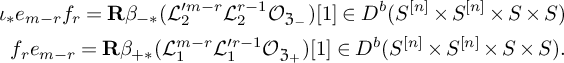 $$ \begin{align*} \iota_{*}e_{m-r}f_{r}=\mathbf{R}\beta_{-*}(\mathcal{L}_2^{\prime m-r}\mathcal{L}_2^{r-1}\mathcal{O}_{\mathfrak{Z}_{-}})[1]\in D^b(S^{[n]}\times S^{[n]}\times S \times S) \\ f_re_{m-r}=\mathbf{R}\beta_{+*}(\mathcal{L}_1^{m-r}\mathcal{L}_1^{\prime r-1}\mathcal{O}_{\mathfrak{Z}_{+}})[1]\in D^b(S^{[n]}\times S^{[n]}\times S \times S). \end{align*} $$
By Proposition 4.6, $\mathbf {R}\alpha _{-*}\mathcal {O}_{\mathfrak {Y}}=\mathcal {O}_{\mathfrak {Z}_-}$
, and by Theorem 4.3
$\mathbf {R}\alpha _{-*}\mathcal {O}_{\mathfrak {Y}}=\mathcal {O}_{\mathfrak {Z}_-}$
, and by Theorem 4.3
 $$ \begin{align} \iota_{*}e_{m-r}f_r&=\mathbf{R}\theta_*(\mathcal{L}_2^{\prime m-r}\mathcal{L}_2^{r-1}\mathcal{O}_{\mathfrak{Y}})[1] \nonumber \\ &=\mathbf{R}\theta_*(\mathcal{L}_1^{\prime m-r}\mathcal{L}_1^{r-1}\mathcal{O}((m-1)\Delta_{\mathfrak{Y}}))[1]. \end{align} $$
5.2
$a_{m,r}^{k}$
and
$\mathfrak {A}_{m,r}^k$


We recall the short exact sequence
 $$ \begin{align} 0\to \mathcal{O}_{\mathfrak{Y}}(-\Delta_{\mathfrak{Y}})\to \mathcal{O}_{\mathfrak{Y}} \to \mathcal{O}_{\Delta_{\mathfrak{Y}}}\to 0. \end{align} $$
Definition 5.2. For any integer r, we define
 $$ \begin{align*}a_{m,r}^{k}=\mathbf{R}\theta_{*}(\mathcal{L}_{1}^{\prime m-r}\mathcal{L}_{1}^{r-1}\mathcal{O}(k\Delta_{\mathfrak{Y}}))[1].\end{align*} $$
We define the exact triangles
 $$ \begin{align} \mathfrak{A}_{m,r}^k :a_{m,r}^{k-1}\to a_{m,r}^{k} \to \mathbf{R}\Delta_*(\mathbf{R}(p_n\circ q_n)_*\mathcal{L}_{1}^{m-1-k}\mathcal{L}_{2}^k)[1] \to a_{m,r}^{k-1}[1] \end{align} $$
by applying the functor $\mathbf {R}\theta _{*}(-\otimes \mathcal {L}_{1}^{\prime m-r}\mathcal {L}_{1}^{r-1}\mathcal {O}(k\Delta _{\mathfrak {Y}}))[1]$
to (5.2).
$\mathbf {R}\theta _{*}(-\otimes \mathcal {L}_{1}^{\prime m-r}\mathcal {L}_{1}^{r-1}\mathcal {O}(k\Delta _{\mathfrak {Y}}))[1]$
to (5.2).
By (5.1), $\iota _{*}e_{m-r}f_r\cong a_{m,r}^{m-1}$
. Moreover, when
$\iota _{*}e_{m-r}f_r\cong a_{m,r}^{m-1}$
. Moreover, when $m<0$
, by (3.14),
$m<0$
, by (3.14), $\mathbf {R}(p_n\circ q_n)_*\mathcal {L}_{1}^{-1}\mathcal {L}_{2}^m=0$
and
$\mathbf {R}(p_n\circ q_n)_*\mathcal {L}_{1}^{-1}\mathcal {L}_{2}^m=0$
and $\iota _{*}e_{m-r}f_r\cong a_{m,r}^{m-1}\cong a_{m,r}^m$
.
$\iota _{*}e_{m-r}f_r\cong a_{m,r}^{m-1}\cong a_{m,r}^m$
.
5.3
$\mathfrak {B}_{m,r}^{\prime 0}$
and
$\mathfrak {C}_{m,r}^{\prime 0}$


By Example B.9, $\mathbf {R}\alpha _{+*}\mathcal {O}_{\Delta _{\mathfrak {Y}}}=\mathcal {O}_{W_0\cap W_1}$
. Taking the
$\mathbf {R}\alpha _{+*}\mathcal {O}_{\Delta _{\mathfrak {Y}}}=\mathcal {O}_{W_0\cap W_1}$
. Taking the $\mathbf {R}\alpha _{+*}$
functor to the short exact sequence (5.2), we have the short exact sequence
$\mathbf {R}\alpha _{+*}$
functor to the short exact sequence (5.2), we have the short exact sequence
 $$ \begin{align*} 0\to \mathbf{R}\alpha_{+*}\mathcal{O}(-\Delta_{\mathfrak{Y}})\to \mathcal{O}_{W_0}\to \mathcal{O}_{W_0\cap W_1}\to 0. \end{align*} $$
Recalling the short exact sequence in Corollary 3.6:
 $$ \begin{align*}0\to \mathcal{L}\otimes \mathcal{O}_{W_1}\to \mathcal{O}_{W_1}\to \mathcal{O}_{W_0\cap W_1}\to 0.\end{align*} $$
We have the following commutative diagram:

where all rows and columns are short exact sequences. Thus, we have short exact sequences:
 $$ \begin{align} 0\to \mathbf{R}\alpha_{+*}\mathcal{O}(-\Delta_{\mathfrak{Y}})\to \mathcal{O}_{\mathfrak{Z}_+} \to \mathcal{O}_{W_1}\to 0 \end{align} $$
 $$ \begin{align} 0\to \mathcal{L}_1\mathcal{O}_{S^{[n,n+1]}}\to \mathcal{O}_{\mathfrak{Z}_{+}} \to \mathcal{O}_{W_0}\to 0. \end{align} $$
Taking the functor $\mathbf {R}\beta _{+*}(-\otimes \mathcal {L}_{1}^{\prime m-r}\mathcal {L}_{1}^{r-1})[1]$
to (5.4) and (5.5), respectively, we get the exact triangles
$\mathbf {R}\beta _{+*}(-\otimes \mathcal {L}_{1}^{\prime m-r}\mathcal {L}_{1}^{r-1})[1]$
to (5.4) and (5.5), respectively, we get the exact triangles
 $$ \begin{align} & \mathfrak{C}_{m,r}^{\prime 0}:a_{m,r}^{-1}\to f_{r}e_{m-r} \to \mathbf{R}\Delta_*(\mathbf{R}p_{n*} \mathcal{L}^{m-1})[1] \to a_{m,r}^{-1}[1] \end{align} $$
 $$ \begin{align} & \mathfrak{B}_{m,r}^{\prime 0}: \mathbf{R}\Delta_*(\mathbf{R}p_{n*}\mathcal{L}^{m})[1] \to f_{r}e_{m-r} \to a_{m,r}^0 \to \mathbf{R}\Delta_*(\mathbf{R}p_{n*}\mathcal{L}^{m})[2]. \end{align} $$
5.4
$\mathfrak {B}_{m,r}^k$
and
$\mathfrak {C}_{m,r}^k$


Definition 5.3. When $m>0$
, we define
$m>0$
, we define $b_{m.r}^k\in D^{b}(S^{[n]}\times S^{[n]}\times S\times S)$
and natural transforms
$b_{m.r}^k\in D^{b}(S^{[n]}\times S^{[n]}\times S\times S)$
and natural transforms $\mathfrak {B}_{m,r}^k:b_{m,r}^{k}\to b_{m,r}^{k+1}$
by
$\mathfrak {B}_{m,r}^k:b_{m,r}^{k}\to b_{m,r}^{k+1}$
by
 $$ \begin{align} b_{m,r}^k:= \begin{cases} f_{r}e_{m-r} & k=0\\ a_{m,r}^{k-1} & 1\leq k\leq m \end{cases} \end{align} $$
 $$ \begin{align} \mathfrak{B}_{m,r}^k:= \begin{cases} \mathfrak{B}_{m,r}^{\prime 0} & k=0\\ \mathfrak{A}_{m,r}^{k}& 1\leq k\leq m-1. \end{cases} \end{align} $$
We have $b_{m,r}^{0}=f_re_{m-r}$
and
$b_{m,r}^{0}=f_re_{m-r}$
and $b_{m,r}^{m}=\iota _{*}e_{m-r}f_r$
.
$b_{m,r}^{m}=\iota _{*}e_{m-r}f_r$
.
When $m<0$
, we define
$m<0$
, we define $c_{m,r}^k\in D^{b}(S^{[n]}\times S^{[n]}\times S\times S)$
and
$c_{m,r}^k\in D^{b}(S^{[n]}\times S^{[n]}\times S\times S)$
and $\mathfrak {C}_{m,r}^k:c_{m,r}^{k-1}\to c_{m,r}^{k}$
by
$\mathfrak {C}_{m,r}^k:c_{m,r}^{k-1}\to c_{m,r}^{k}$
by
 $$ \begin{align} c_{m,r}^k= \begin{cases} f_{r}e_{m-r} & k=0\\ a_{m,r}^k & m\leq k\leq -1 \end{cases} \end{align} $$
 $$ \begin{align} \mathfrak{C}_{m,r}^k= \begin{cases} \mathfrak{C}_{m,r}^{\prime 0} & k=0 \\ \mathfrak{A}_{m,r}^k & m+1 \leq k \leq -1. \end{cases} \end{align} $$
We have $f_re_{m-r}=c_{m,r}^{0}$
and
$f_re_{m-r}=c_{m,r}^{0}$
and $\iota _{*}e_{m-r}f_r=c_{m,r}^{m}$
.
$\iota _{*}e_{m-r}f_r=c_{m,r}^{m}$
.
Proof of Theorem 5.1
When $m>0$
, we only need to prove that the cone of
$m>0$
, we only need to prove that the cone of $\mathfrak {B}_{m,r}^k$
is
$\mathfrak {B}_{m,r}^k$
is $\mathbf {R}\Delta _*(h_{m,k}^+)$
and the cone of
$\mathbf {R}\Delta _*(h_{m,k}^+)$
and the cone of $\mathfrak {C}_{m,r}^k$
is
$\mathfrak {C}_{m,r}^k$
is $\mathbf {R}\Delta _*(h_{m,k}^-)$
. It follows from (5.3), (5.6) and (5.7).
$\mathbf {R}\Delta _*(h_{m,k}^-)$
. It follows from (5.3), (5.6) and (5.7).
When $m=0$
,
$m=0$
,
 $$ \begin{align*} e_{-r}f_r=\mathbf{R}\beta_{+*}(\mathbf{R}\alpha_{+*}(\mathcal{L}_1^{\prime -r}\mathcal{L}_1^{r-1}\mathcal{O}(-\Delta_{\mathfrak{Y}}))). \end{align*} $$
We have the short exact sequence:
 $$ \begin{align} 0\to \mathcal{L}_1^{\prime -r}\mathcal{L}_1^{r-1}\mathcal{O}_{\mathfrak{Z}_+}\to \mathcal{L}_1^{\prime -r}\mathcal{L}_1^{r-1}(\mathcal{O}_{W_0}\oplus\mathcal{O}_{W_1})\to \mathcal{L}^{-1}\mathcal{O}_{W_0\cap W_1}\to 0, \end{align} $$
and
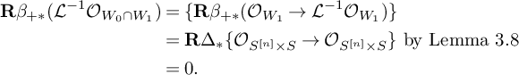 $$ \begin{align*} \mathbf{R}\beta_{+*}(\mathcal{L}^{-1}\mathcal{O}_{W_0\cap W_1})&=\{\mathbf{R}\beta_{+*}(\mathcal{O}_{W_1}\to \mathcal{L}^{-1}\mathcal{O}_{W_1})\} \\ &=\mathbf{R}\Delta_{*}\{\mathcal{O}_{S^{[n]}\times S}\to \mathcal{O}_{S^{[n]}\times S}\} \text{ by Lemma~3.8 }\\ &=0. \end{align*} $$
By (5.4) and (5.12), we have isomorphisms
 $$ \begin{align*} & f_{r}e_{-r}\cong \mathbf{R}\beta_{+*}\mathcal{L}_1^{\prime -r}\mathcal{L}_1^{r-1}(\mathcal{O}_{W_0})[1]\oplus\mathcal{O}_{\Delta}[1] \\ & e_{-r}f_{r}\cong \mathbf{R}\beta_{+*}\mathcal{L}_1^{\prime -r}\mathcal{L}_1^{r-1}(\mathcal{O}_{W_0})[1].\\[-40pt] \end{align*} $$
6 Extension classes between
$h_{m,k}^{\pm }$

When $m>0$
, the composition of
$m>0$
, the composition of $\mathfrak {B}_{m,r}^k$
and
$\mathfrak {B}_{m,r}^k$
and $\mathfrak {B}_{m,r}^{k+1}$
in Theorem 5.1 induces an extension of
$\mathfrak {B}_{m,r}^{k+1}$
in Theorem 5.1 induces an extension of $\mathbf {R}\Delta _*h_{m,k-1}^{+}$
and
$\mathbf {R}\Delta _*h_{m,k-1}^{+}$
and $\mathbf {R}\Delta _*h_{m,k}^{+}$
, that is an extension class of
$\mathbf {R}\Delta _*h_{m,k}^{+}$
, that is an extension class of
 $$ \begin{align*}Hom(\mathbf{R}\Delta_*h_{m,k}^{+},\mathbf{R}\Delta_*h_{m,k-1}^{+}[1]).\end{align*} $$
Similarly, when $m<0$
, there is also an extension class of
$m<0$
, there is also an extension class of
 $$ \begin{align*}Hom(\mathbf{R}\Delta_*h_{m,k}^{-},\mathbf{R}\Delta_*h_{m,k-1}^{-}[1])\end{align*} $$
which relies on $m,k,r$
. The purpose of this section is to study the above extension classes. First we recall the Hochschild-Kostant-Rosenberg theorem (short for HKR theorem). Let
$m,k,r$
. The purpose of this section is to study the above extension classes. First we recall the Hochschild-Kostant-Rosenberg theorem (short for HKR theorem). Let $f:X\to Y$
be a regular embedding of smooth varieties. On X, we have the following short exact sequence
$f:X\to Y$
be a regular embedding of smooth varieties. On X, we have the following short exact sequence
 $$ \begin{align*}0\to N_{Y/X}^{{\vee}}\xrightarrow{\iota_{Y/X}}T^{*}Y|_{X}\to T^{*}X\to 0.\end{align*} $$
Let $g:T^{*}Y\to N_{Y/X}^{{\vee }}$
be a splitting of the above short exact sequence, that is
$g:T^{*}Y\to N_{Y/X}^{{\vee }}$
be a splitting of the above short exact sequence, that is $g{\circ }\iota _{Y/X}=id$
.
$g{\circ }\iota _{Y/X}=id$
.
Theorem 6.1 (HKR isomorphism, Theorem 1.4 and Section 1.11 of [Reference Arinkin and Căldăraru1], see Theorem C.10 for the precise formulation).
The splitting g induces a canonical isomorphism
 $$ \begin{align*}\tau_{N_{Y/X}^{{\vee}}}^{F,G}:\mathbf{R}Hom_{X}(F{\otimes}^{\mathbf{L}}(\bigoplus_{j=0}^{\infty}{\wedge}^{j}N_{Y/X}^{{\vee}}),G){\cong}\mathbf{R}Hom_{Y}(\mathbf{R}f_{*}F,\mathbf{R}f_{*}G)\end{align*} $$
which is functorial respect to $F,G\in D(X)$
.
$F,G\in D(X)$
.
Remark 6.2. The isomorphism $\tau _{N_{X/Y}^{{\vee }}}^{F,G}$
depends on the choice of the splitting g. For a different choice of g, the difference of the isomorphism
$\tau _{N_{X/Y}^{{\vee }}}^{F,G}$
depends on the choice of the splitting g. For a different choice of g, the difference of the isomorphism $\tau _{N_{X/Y}^{{\vee }}}^{F,G}$
is represented by a transition matrix in Proposition 3.7 of [Reference Huang13].
$\tau _{N_{X/Y}^{{\vee }}}^{F,G}$
is represented by a transition matrix in Proposition 3.7 of [Reference Huang13].
Now we consider the diagonal embedding $\Delta :S^{[n]}{\times }S\to S^{[n]}{\times }S^{[n]}{\times }S{\times }S$
. Then
$\Delta :S^{[n]}{\times }S\to S^{[n]}{\times }S^{[n]}{\times }S{\times }S$
. Then $T^{*}(S^{[n]}{\times }S^{[n]}{\times }S{\times }S)|_{\Delta }=T^{*}(S^{[n]}{\times }S){\oplus }T^{*}(S^{[n]}{\times }S)$
, where the conormal bundle is
$T^{*}(S^{[n]}{\times }S^{[n]}{\times }S{\times }S)|_{\Delta }=T^{*}(S^{[n]}{\times }S){\oplus }T^{*}(S^{[n]}{\times }S)$
, where the conormal bundle is
 $$ \begin{align*}T^{*}(S^{[n]}{\times}S){\cong}\{(x,-x)\in T^{*}(S^{[n]}{\times}S){\oplus}T^{*}(S^{[n]}{\times}S)\}.\end{align*} $$
We take the split
 $$ \begin{align} (T^{*}\Delta)^{-1}:T^{*}(S^{[n]}{\times}S){\oplus}T^{*}(S^{[n]}{\times}S)\to T^{*}(S^{[n]}{\times}S) \end{align} $$
which maps $(a,b)$
to
$(a,b)$
to $(\frac {1}{2}(a-b),\frac {1}{2}(b-a))$
and, hence, induce isomorphisms
$(\frac {1}{2}(a-b),\frac {1}{2}(b-a))$
and, hence, induce isomorphisms
 $$ \begin{align*} Hom(\mathbf{R}\Delta_*h_{m,k}^{+},\mathbf{R}\Delta_*h_{m,k-1}^{+}[1])=\bigoplus_{j=0}^{\infty} Hom_{S^{[n]}{\times}S}(h_{m,k}^+\otimes \wedge^jT^*(S^{[n]}\times S),h_{m,k-1}^+[1-j]),\\ Hom(\mathbf{R}\Delta_*h_{m,k}^{-},\mathbf{R}\Delta_*h_{m,k-1}^{-}[1])=\bigoplus_{j=0}^{\infty} Hom_{S^{[n]}{\times}S}(h_{m,k}^{-}\otimes \wedge^jT^*(S^{[n]}\times S),h_{m,k-1}^{-}[1-j]). \end{align*} $$
In this section, we will be explicitly computing the above extension classes and prove that
Proposition 6.3. The extension class in $Hom(\mathbf {R}\Delta _*h_{m,k}^{+},\mathbf {R}\Delta _*h_{m,k-1}^{+}[1])$
is
$Hom(\mathbf {R}\Delta _*h_{m,k}^{+},\mathbf {R}\Delta _*h_{m,k-1}^{+}[1])$
is
 $$ \begin{align*}(\mathfrak{F}_{m,k,r}^{+},\mathfrak{H}_{m,k}^{+},0,0,\cdots)\end{align*} $$
and the extension class in $Hom(\mathbf {R}\Delta _*h_{m,k}^{-},\mathbf {R}\Delta _*h_{m,k-1}^{-}[1])$
is
$Hom(\mathbf {R}\Delta _*h_{m,k}^{-},\mathbf {R}\Delta _*h_{m,k-1}^{-}[1])$
is
 $$ \begin{align*}(\mathfrak{F}_{m,k,r}^{-},\mathfrak{H}_{m,k}^-,0,0,\cdots),\end{align*} $$
where $\mathfrak {F}_{m,k,r}^{+}$
,
$\mathfrak {F}_{m,k,r}^{+}$
, $\mathfrak {F}_{m,k,r}^{-}$
,
$\mathfrak {F}_{m,k,r}^{-}$
, $\mathfrak {H}_{m,k}^{+}$
and
$\mathfrak {H}_{m,k}^{+}$
and $\mathfrak {H}_{m,k}^{-}$
will be defined in Definition 6.7. The classes
$\mathfrak {H}_{m,k}^{-}$
will be defined in Definition 6.7. The classes $\mathfrak {H}_{m,k}^{+}$
and
$\mathfrak {H}_{m,k}^{+}$
and $\mathfrak {H}_{m,k}^{-}$
only depend on
$\mathfrak {H}_{m,k}^{-}$
only depend on $m,k$
but not r.
$m,k$
but not r.
Proposition 6.3 will be proved later in this section.
6.1 A morphism
$s: \mathcal {L}_{1}^{-1} \mathcal {L}_{2} \to (p_n\circ q_n)^{*}T(S^{[n]}\times S)$

By restricting $\theta :\mathfrak {Y}\to S^{[n]}\times S^{[n]}\times S\times S$
to the diagonal of
$\theta :\mathfrak {Y}\to S^{[n]}\times S^{[n]}\times S\times S$
to the diagonal of $S^{[n]}\times S^{[n]}\times S\times S$
, we get the Cartesian diagram:
$S^{[n]}\times S^{[n]}\times S\times S$
, we get the Cartesian diagram:

and the normal bundle of $S^{[n]}\times S$
in
$S^{[n]}\times S$
in $S^{[n]}\times S^{[n]}\times S\times S$
is
$S^{[n]}\times S^{[n]}\times S\times S$
is $T(S^{[n]}\times S)$
. Thus, the diagram (6.2) induces a morphism of short exact sequences:
$T(S^{[n]}\times S)$
. Thus, the diagram (6.2) induces a morphism of short exact sequences:

where $N_{\mathfrak {Y}/\Delta _{\mathfrak {Y}}}{\cong }\mathcal {L}_1^{-1}\mathcal {L}_2$
. The purpose of this subsection is to construct a split
$N_{\mathfrak {Y}/\Delta _{\mathfrak {Y}}}{\cong }\mathcal {L}_1^{-1}\mathcal {L}_2$
. The purpose of this subsection is to construct a split $\lambda :{\mathcal {L}}_{1}^{-1}{\mathcal {L}}_{2}\to T{\mathfrak {Y}}|_{S^{n-1,n,n+1}}$
which is compatible with the splitting of tangent bundle (or cotangent bundle) in (6.1) and give an explicit formulation of
$\lambda :{\mathcal {L}}_{1}^{-1}{\mathcal {L}}_{2}\to T{\mathfrak {Y}}|_{S^{n-1,n,n+1}}$
which is compatible with the splitting of tangent bundle (or cotangent bundle) in (6.1) and give an explicit formulation of $s'$
in Proposition 6.6. First we recall the description of the tangent space of
$s'$
in Proposition 6.6. First we recall the description of the tangent space of $S^{[n-1,n,n+1]}$
and
$S^{[n-1,n,n+1]}$
and $\mathfrak {Y}$
in Proposition 5.28 of [Reference Neguţ26]: we consider a closed point
$\mathfrak {Y}$
in Proposition 5.28 of [Reference Neguţ26]: we consider a closed point $t\in S^{[n-1,n,n+1]}$
corresponds to two short exact sequences of coherent sheaves on S:
$t\in S^{[n-1,n,n+1]}$
corresponds to two short exact sequences of coherent sheaves on S:
 $$ \begin{align*} 0\to \mathcal{I}_{n}\xrightarrow{i_n} \mathcal{I}_{n-1}\xrightarrow{j_n} k_x \to 0 & \quad 0\to \mathcal{I}_{n+1}\xrightarrow{i_{n+1}} \mathcal{I}_{n}\xrightarrow{j_{n+1}} k_x \to 0. \end{align*} $$
Let V be the vector space of pairs $\{(w_0,w_1)\in Ext^1(\mathcal {I}_{n-1},\mathcal {I}_{n-1})\oplus Ext^1(\mathcal {I}_{n},\mathcal {I}_n)\}$
, such that
$\{(w_0,w_1)\in Ext^1(\mathcal {I}_{n-1},\mathcal {I}_{n-1})\oplus Ext^1(\mathcal {I}_{n},\mathcal {I}_n)\}$
, such that $w_0,w_1$
map to the same element of
$w_0,w_1$
map to the same element of $Ext^1(\mathcal {I}_n,\mathcal {I}_{n-1})$
. By the proof of Proposition 5.28 of [Reference Neguţ26], elements in V are in 1-1 correspondence with the commutative diagrams of short exact sequences:
$Ext^1(\mathcal {I}_n,\mathcal {I}_{n-1})$
. By the proof of Proposition 5.28 of [Reference Neguţ26], elements in V are in 1-1 correspondence with the commutative diagrams of short exact sequences:

and, thus, induce a morphism $dp_S^1:V\to Ext^1(k_x,k_x)$
. Let
$dp_S^1:V\to Ext^1(k_x,k_x)$
. Let $V'$
be the vector space of pairs
$V'$
be the vector space of pairs
 $$ \begin{align*} \{(w_1',w_2)\in Ext^1(\mathcal{I}_{n},\mathcal{I}_n)\oplus Ext^1(\mathcal{I}_{n+1},\mathcal{I}_{n+1})\}, \end{align*} $$
such that $w_1',w_2$
map to the same element of
$w_1',w_2$
map to the same element of $Ext^1(\mathcal {I}_{n},\mathcal {I}_{n+1})$
. Then elements in
$Ext^1(\mathcal {I}_{n},\mathcal {I}_{n+1})$
. Then elements in $V'$
are in 1-1 correspondence with the commutative diagrams of short exact sequences:
$V'$
are in 1-1 correspondence with the commutative diagrams of short exact sequences:

and, thus, also induces a morphism $dp_S^2:V'\to Ext^1(k_x,k_x)$
.
$dp_S^2:V'\to Ext^1(k_x,k_x)$
.
Consider the natural morphism:
 $$ \begin{align*} \hat{s}_1: Hom(\mathcal{I}_n,k_x)\otimes Ext^1(k_x,\mathcal{I}_n)\to Ext^1(\mathcal{I}_n,\mathcal{I}_n) \\ \hat{s}_2: Hom(\mathcal{I}_n,k_x)\otimes Ext^1(k_x,\mathcal{I}_n)\to Ext^1(k_x,k_x), \end{align*} $$
and the short exact sequences
 $$ \begin{align*} Hom(\mathcal{I}_n,k_x)\xrightarrow{\hat{s}_1(-\otimes r_2)} Ext^1(\mathcal{I}_n,\mathcal{I}_n)\to Ext^1(\mathcal{I}_n,\mathcal{I}_{n-1}) \\ Ext^{1}(k_x,\mathcal{I}_n)\xrightarrow{\hat{s}_1(r_1\otimes -)}Ext^1(\mathcal{I}_n,\mathcal{I}_n)\to Ext^1(\mathcal{I}_{n+1},\mathcal{I}_n). \end{align*} $$
For any element $u\in Hom(\mathcal {I}_n,k_x)$
,
$u\in Hom(\mathcal {I}_n,k_x)$
, $(\hat {s}_1(u\otimes r_2),0)\in V$
. Moreover, by diagram chasing (we left it to interested readers)
$(\hat {s}_1(u\otimes r_2),0)\in V$
. Moreover, by diagram chasing (we left it to interested readers)
 $$ \begin{align} dp_S^1(\hat{s}_1(u\otimes r_2),0)=\hat{s}_2(u\otimes r_2). \end{align} $$
Similarly, for any element $v\in Ext^1(k_x,\mathcal {I}_n)$
,
$v\in Ext^1(k_x,\mathcal {I}_n)$
, $(0,\hat {s}_1(r_1\otimes v))\in V'$
and
$(0,\hat {s}_1(r_1\otimes v))\in V'$
and
 $$ \begin{align} dp_S^2(0,\hat{s}_1(r_1\otimes v))=\hat{s}_2(r_1\otimes v). \end{align} $$
Lemma 6.4 (Proposition 5.28 of [Reference Neguţ26]).
The tangent space $T_{t}\mathfrak {Y}$
is the space of
$T_{t}\mathfrak {Y}$
is the space of $(w_0,w_1,w_1',w_2,u,v)$
in
$(w_0,w_1,w_1',w_2,u,v)$
in
 $$ \begin{align*}&Ext^1(\mathcal{I}_{n-1},\mathcal{I}_{n-1})\oplus Ext^{1}(\mathcal{I}_n,\mathcal{I}_n)\oplus Ext^{1}(\mathcal{I}_n,\mathcal{I}_n)\oplus Ext^{1}(\mathcal{I}_{n+1},\mathcal{I}_{n+1})\oplus Ext^1(k_x,k_x)\\&\quad\oplus Ext^1(k_x,k_x),\end{align*} $$
such that
-
(1)
$(w_0,w_1)$
and
$(w_0,w_1')$
are in V. -
(2)
$(w_1,w_2)$
and
$(w_1',w_2)$
are in
$V'$
. -
(3)
$dp_S^1(w_0,w_1)=dp_S^2(w_1',w_2)=u$
, -
(4)
$dp_S^1(w_0,w_1')=dp_S^2(w_1,w_2)=v$
.


The tangent space $T_{t}S^{[n-1,n,n+1]}$
consists of subspace of
$T_{t}S^{[n-1,n,n+1]}$
consists of subspace of $T_{t}\mathfrak {Y}$
, such that
$T_{t}\mathfrak {Y}$
, such that $w_{1}=w_{1}'$
and
$w_{1}=w_{1}'$
and $u=v$
.
$u=v$
.
Corollary 6.5. The morphism $\lambda _{t}:T_{t}{\mathfrak {Y}}\to T_{t}{\mathfrak {Y}}:(w_0,w_1,w_1',w_2,u,v)\to (0,w_1'-w_1,w_1'-w_1,0,u-v,v-u)$
induces a splitting
$\lambda _{t}:T_{t}{\mathfrak {Y}}\to T_{t}{\mathfrak {Y}}:(w_0,w_1,w_1',w_2,u,v)\to (0,w_1'-w_1,w_1'-w_1,0,u-v,v-u)$
induces a splitting $\lambda :{\mathcal {L}}_{1}^{-1}{\mathcal {L}}_{2}\to T{\mathfrak {Y}}|_{S^{[n-1,n,n+1]}}$
which is compatible with (6.1). Moreover, under the splitting
$\lambda :{\mathcal {L}}_{1}^{-1}{\mathcal {L}}_{2}\to T{\mathfrak {Y}}|_{S^{[n-1,n,n+1]}}$
which is compatible with (6.1). Moreover, under the splitting $\lambda $
,
$\lambda $
, ${\mathcal {L}}_{1}{\mathcal {L}}_{2}^{-1}|_{t}$
is
${\mathcal {L}}_{1}{\mathcal {L}}_{2}^{-1}|_{t}$
is
 $$ \begin{align*}\{(w,v)\in Ext^{1}({\mathcal{I}}_{n},{\mathcal{I}}_{n}){\oplus}Ext^{1}(k_{x},k_{x})|(0,w)\in V,(w,0)\in V',dp_{S}^{1}(0,w)=dp_{S}^{2}(w,0)=u\}.\end{align*} $$
Proof. If $(w_0,w_1,w_1',w_2,u,v)$
is in the tangent space, then so is
$(w_0,w_1,w_1',w_2,u,v)$
is in the tangent space, then so is
 $$ \begin{align*}\frac{(2w_0,w_1+w_1',w_1+w_1',2w_2,u+v,u+v)}{2} \text{ and } (0,w_1'-w_1,w_1-w_1',0,u-v,v-u).\end{align*} $$
Hence, the tangent space $T_t\mathfrak {Y}$
decomposes into a direct sum of two subspaces: the subspace
$T_t\mathfrak {Y}$
decomposes into a direct sum of two subspaces: the subspace $w_1=w_1'$
, which is
$w_1=w_1'$
, which is $T_tS^{[n-1,n,n+1]}$
, and the subspace N, which consists of elements
$T_tS^{[n-1,n,n+1]}$
, and the subspace N, which consists of elements $(w_1,u)\in Ext^{1}(\mathcal {I}_n,\mathcal {I}_n)\oplus Ext^{1}(k_x,k_x)$
, such that
$(w_1,u)\in Ext^{1}(\mathcal {I}_n,\mathcal {I}_n)\oplus Ext^{1}(k_x,k_x)$
, such that
-
(1)
$w_1$
maps to
$0$
in
$Ext^{1}(\mathcal {I}_{n}, \mathcal {I}_{n-1})$
and
$Ext^{1}(\mathcal {I}_{n+1}, \mathcal {I}_{n}),$
-
(2)
$dp_S^1(w_1,0)=dp_S^2(0,w_1)=u.$


We define the morphism $\lambda _{t}$
just to be the projection to N, and it induces a splitting
$\lambda _{t}$
just to be the projection to N, and it induces a splitting $\lambda :{\mathcal {L}}_{1}^{-1}{\mathcal {L}}_{2}\to T{\mathfrak {Y}}|_{S^{[n-1,n,n+1]}}$
.
$\lambda :{\mathcal {L}}_{1}^{-1}{\mathcal {L}}_{2}\to T{\mathfrak {Y}}|_{S^{[n-1,n,n+1]}}$
.
Now we give an explicit description of $s'$
. We first construct two canonical morphisms:
$s'$
. We first construct two canonical morphisms:
 $$ \begin{align} s_1:\mathcal{L}_1^{-1}\mathcal{L}_2\to (p_n\circ q_n)^*TS^{[n]}\quad s_2:\mathcal{L}_1^{-1}\mathcal{L}_2\to (p_n\circ q_n)^*(TS). \end{align} $$
Let $\pi :S^{[n-1,n,n+1]}\times S\to S^{[n-1,n,n+1]}$
be the projection morphism and
$\pi :S^{[n-1,n,n+1]}\times S\to S^{[n-1,n,n+1]}$
be the projection morphism and $\Gamma $
be the graph of the projection map to S. Then there exists short exact sequences:
$\Gamma $
be the graph of the projection map to S. Then there exists short exact sequences:
 $$ \begin{align*}0\to \mathcal{I}_{n+1}\to \mathcal{I}_n\to \pi^*\mathcal{L}_{1}\otimes \mathcal{O}_{\Gamma}\to 0\quad 0\to \mathcal{I}_{n}\to \mathcal{I}_{n-1}\to \pi^*\mathcal{L}_{2}\otimes \mathcal{O}_{\Gamma}\to 0\end{align*} $$
which induce two global sections:
 $$ \begin{align*} r_1:\mathcal{L}_1^{-1}\to \mathcal{H}om_{\pi}(\mathcal{I}_n,\mathcal{O}_{\Gamma}), \quad r_2:\mathcal{L}_2\to \mathcal{E}xt^1_{\pi}(\mathcal{O}_{\Gamma},\mathcal{I}_{n}). \end{align*} $$
Let $\text {proj}_n:S^{[n]}\times S\to S^{[n]}$
be the projection map and
$\text {proj}_n:S^{[n]}\times S\to S^{[n]}$
be the projection map and $\Gamma _n$
be the graph of the projection map from
$\Gamma _n$
be the graph of the projection map from $S^{[n]}\times S\to S$
. Then
$S^{[n]}\times S\to S$
. Then
 $$ \begin{align*} (p_n\circ q_n)^*TS^{[n]}&=(p_n\circ q_n)^*\mathcal{E}xt_{\text{proj}_n}^1(\mathcal{I}_n,\mathcal{I}_n)\\ &=\mathcal{E}xt^1_{\pi}(\mathcal{I}_n,\mathcal{I}_n)\\ (p_n\circ q_n)^*TS&=\mathcal{E}xt^1_{\pi}(\mathcal{O}_{\Gamma},\mathcal{O}_{\Gamma}) \end{align*} $$
by the flat base change theorem. With the composition of the following two natural homomorphisms:
 $$ \begin{align*} \mathcal{E}xt^1_{\pi}(\mathcal{O}_{\Gamma},\mathcal{I}_n)\otimes \mathcal{H}om_{\pi}(\mathcal{I}_n, \mathcal{O}_{\Gamma}) \to \mathcal{E}xt^1_{\pi}(\mathcal{I}_n,\mathcal{I}_n)=(p_n\circ q_n)^*TS^{[n]} \\ \mathcal{H}om_{\pi}(\mathcal{I}_n,\mathcal{O}_{\Gamma})\otimes \mathcal{E}xt^1_{\pi}(\mathcal{O}_{\Gamma},\mathcal{I}_n)\to \mathcal{E}xt^1_{\pi}(\mathcal{O}_{\Gamma},\mathcal{O}_{\Gamma})=(p_n\circ q_n)^*TS, \end{align*} $$
we get the two canonical morphisms in (6.6)
 $$ \begin{align*} s_1:\mathcal{L}_1^{-1}\mathcal{L}_2\to (p_n\circ q_n)^*TS^{[n]}\quad s_2:\mathcal{L}_1^{-1}\mathcal{L}_2\to (p_n\circ q_n)^*(TS). \end{align*} $$
Let
 $$ \begin{align*} s=(s_1,s_2):\mathcal{L}_1^{-1}\mathcal{L}_2\to (p_n\circ q_n)^*T(S^{[n]}\times S). \end{align*} $$

Proof. A closed point t on $S^{[n-1,n,n+1]}$
corresponds to two short exact sequences of coherent sheaves on S:
$S^{[n-1,n,n+1]}$
corresponds to two short exact sequences of coherent sheaves on S:
 $$ \begin{align*} 0\to \mathcal{I}_{n}\xrightarrow{i_n} \mathcal{I}_{n-1}\xrightarrow{j_n} k_x \to 0 & \quad 0\to \mathcal{I}_{n+1}\xrightarrow{i_{n+1}} \mathcal{I}_{n}\xrightarrow{j_{n+1}} k_x \to 0, \end{align*} $$
which induces $r_1\in Hom(\mathcal {I}_n,k_x)$
and
$r_1\in Hom(\mathcal {I}_n,k_x)$
and $r_2\in Ext^1(k_x,\mathcal {I}_n)$
. The image of s is
$r_2\in Ext^1(k_x,\mathcal {I}_n)$
. The image of s is $(\hat {s}_1(r_1\otimes r_2),\hat {s}_2(r_1\otimes r_2))$
, and we only need to prove that it is also the image of N in the proof of Corollary 6.5. It follows from the fact that
$(\hat {s}_1(r_1\otimes r_2),\hat {s}_2(r_1\otimes r_2))$
, and we only need to prove that it is also the image of N in the proof of Corollary 6.5. It follows from the fact that
 $$ \begin{align*}dp_S^1(\hat{s}_1(r_1\otimes r_2),0)=dp_S^2(0,\hat{s}_1(r_1\otimes r_2))=\hat{s}_2(r_1\otimes r_2)\end{align*} $$
6.2 The definition of
$\mathfrak {F}_{m,k,r}^{+},\mathfrak {H}_{m,k}^{\pm }$

We recall the Cartesian diagram (6.2)

Consider the dual of s
 $$ \begin{align*}s^{\vee}:(p_n\circ q_n)^*T^*(S^{[n]}\times S)\to \mathcal{L}_1\mathcal{L}_2^{-1}\end{align*} $$
and the splitting $\lambda ^{{\vee }}$
in Corollary 6.5. We define
$\lambda ^{{\vee }}$
in Corollary 6.5. We define
 $$ \begin{align} \tau_{m}^k:\mathbf{R}(p_n\circ q_n)_*\mathcal{L}_1^{m-1-k}\mathcal{L}_2^k\otimes^{L} T^*(S^{[n]}\times S)\to \mathbf{R}(p_n\circ q_n)_*\mathcal{L}_1^{m-k}\mathcal{L}_2^{k-1} \end{align} $$
as $\mathbf {R}(p_{n}{\circ }q_{n})_{*}(s^{{\vee }}{\otimes }{\mathcal {L}}_{1}^{m-k-1}{\mathcal {L}}_{2}^{k})$
.
$\mathbf {R}(p_{n}{\circ }q_{n})_{*}(s^{{\vee }}{\otimes }{\mathcal {L}}_{1}^{m-k-1}{\mathcal {L}}_{2}^{k})$
.
On the other hand, we recall the definition of Definition 5.2
 $$ \begin{align*}a_{m,r}^{k}=\mathbf{R}\theta_{*}(\mathcal{L}_{1}^{\prime m-r}\mathcal{L}_{1}^{r-1}\mathcal{O}(k\Delta_{\mathfrak{Y}}))[1].\end{align*} $$
By Lemma C.8, the splitting $\lambda $
identify an isomorphism between the first order infinitesimal neighborhood of
$\lambda $
identify an isomorphism between the first order infinitesimal neighborhood of $\Delta _{{\mathfrak {Y}}}$
in
$\Delta _{{\mathfrak {Y}}}$
in ${\mathfrak {Y}}$
with
${\mathfrak {Y}}$
with $Spec_{S^{[n-1,n,n+1]}}({\mathcal {O}}_{S^{[n-1,n,n+1]}}{\oplus }{\mathcal {L}}_{1}{\mathcal {L}}_{2}^{-1})$
. We denote
$Spec_{S^{[n-1,n,n+1]}}({\mathcal {O}}_{S^{[n-1,n,n+1]}}{\oplus }{\mathcal {L}}_{1}{\mathcal {L}}_{2}^{-1})$
. We denote $\alpha _{m,r}^{k}$
as the Bass-Quillen class (see Appendix C.3 for the definition) of
$\alpha _{m,r}^{k}$
as the Bass-Quillen class (see Appendix C.3 for the definition) of $a_{m,r}^{k}$
when restricting to
$a_{m,r}^{k}$
when restricting to $Spec_{S^{[n-1,n,n+1]}}({\mathcal {O}}_{S^{[n-1,n,n+1]}}{\oplus }{\mathcal {L}}_{1}{\mathcal {L}}_{2}^{-1})$
.
$Spec_{S^{[n-1,n,n+1]}}({\mathcal {O}}_{S^{[n-1,n,n+1]}}{\oplus }{\mathcal {L}}_{1}{\mathcal {L}}_{2}^{-1})$
.
By Lemma 3.9,
 $$ \begin{align*}Rq_{n*}(\mathcal{L}_1^{m-1})=\{\mathcal{L}^m\to \mathcal{L}^{m-1}\}\end{align*} $$
is the cone of $\mathcal {L}^m$
to
$\mathcal {L}^m$
to $\mathcal {L}^{m-1}$
. Hence, we have exact triangles
$\mathcal {L}^{m-1}$
. Hence, we have exact triangles
 $$ \begin{align} Rp_{n*}\mathcal{L}^m\to Rp_{n*}\mathcal{L}^{m-1}\xrightarrow{\mu_m} R(p_n\circ q_n)_*(\mathcal{L}_1^{m-1}) \xrightarrow{\nu_m}Rp_{n*}\mathcal{L}^m[1]. \end{align} $$
Definition 6.7. When $m\geq k> 0$
, we define
$m\geq k> 0$
, we define
 $$ \begin{align*}\mathfrak{H}_{m,k}^+:h_{m,k}^+\otimes T^*(S^{[n]}\times S)\to h_{m,k-1}^+\end{align*} $$
by
 $$ \begin{align} \mathfrak{H}_{m,k}^+= \begin{cases} \tau_{m,k} & k>1 \\ \nu_m\circ \tau_{m,0}& k=1, \end{cases} \end{align} $$
and when $m<k\leq 0$
, we define
$m<k\leq 0$
, we define
 $$ \begin{align*}\mathfrak{H}_{m,k}^-:h_{m,k}^-\otimes T^*(S^{[n]}\times S)\to h_{m,k-1}^-\end{align*} $$
by
 $$ \begin{align} \mathfrak{H}_{m,k}^-= \begin{cases} \tau_{m,k} & k<0 \\ \tau_{m,0}\circ \mu_m & k=0. \end{cases} \end{align} $$
Definition 6.8. When $m\geq k> 0$
and r is an integer, we define
$m\geq k> 0$
and r is an integer, we define
 $$ \begin{align*}\mathfrak{F}_{m,k}^+:h_{m,k}^+\otimes T^*(S^{[n]}\times S)\to h_{m,k-1}^+\end{align*} $$
by
 $$ \begin{align} \mathfrak{F}_{m,k}^+= \begin{cases} \alpha_{m,k} & k>1 \\ \nu_m\circ \alpha_{m,0}& k=1, \end{cases} \end{align} $$
and when $m<k\leq 0$
, we define
$m<k\leq 0$
, we define
 $$ \begin{align*}\mathfrak{F}_{m,k}^-:h_{m,k}^-\otimes T^*(S^{[n]}\times S)\to h_{m,k-1}^-\end{align*} $$
by
 $$ \begin{align} \mathfrak{F}_{m,k}^-= \begin{cases} \alpha_{m,k} & k<0 \\ \alpha_{m,0}\circ \mu_m & k=0. \end{cases} \end{align} $$
Proof of Proposition 6.3
We only compute the postive part of the extension and only consider the $k>1$
and the case
$k>1$
and the case $k=1$
follows from the (5.5). The extension class is induced from the short exact sequence on
$k=1$
follows from the (5.5). The extension class is induced from the short exact sequence on $\mathfrak {Y}$
:
$\mathfrak {Y}$
:
 $$ \begin{align*}0\to {\mathcal{L}}_{1}{\mathcal{L}}_{2}^{-1}a_{m,k}^{r}\mathcal{O}_{\Delta_{\mathfrak{Y}}}\to a_{m,k}^{r}\mathcal{O}_{2\Delta_{\mathfrak{Y}}}\to a_{m,k}^{r}\mathcal{O}_{\Delta_{\mathfrak{Y}}}\to 0,\end{align*} $$
where $\mathcal {O}_{2\Delta _{\mathfrak {Y}}}$
is the cokernel of
$\mathcal {O}_{2\Delta _{\mathfrak {Y}}}$
is the cokernel of $\mathcal {O}(-2\Delta _{\mathfrak {Y}})\to \mathcal {O}_{\mathfrak {Y}}$
. Hence, we obtain the extension formula through Theorem C.11.
$\mathcal {O}(-2\Delta _{\mathfrak {Y}})\to \mathcal {O}_{\mathfrak {Y}}$
. Hence, we obtain the extension formula through Theorem C.11.
Appendix A Exterior powers and formal series
Definition A.1. Let V be a locally free sheaf over X, we define the exterior powers of V by
 $$ \begin{align*} \wedge^{\bullet}(xV)=\sum_{i=0}^{\infty}(-x)^i[\wedge^iV], \quad \wedge^{\bullet}(-xV)=\sum_{i=0}^{\infty} x^i[S^iV] \end{align*} $$
as elements in $K(X)[[x]]$
.
$K(X)[[x]]$
.
Definition A.2. For a two term complex of locally free sheaves
 $$ \begin{align*} U:=\{W\xrightarrow{\mathfrak{u}}V\}, \end{align*} $$
we define
 $$ \begin{align*} \wedge^{\bullet}(-xU)=\wedge^{\bullet}(xW)\wedge^{\bullet}(-xV)\qquad \wedge^{\bullet}(xU)=\wedge^{\bullet}(xV)\wedge^{\bullet}(-xW).n \end{align*} $$ $[S^k(U)]$
and
$[S^k(U)]$
and $[\wedge ^k(U)]$
are the
$[\wedge ^k(U)]$
are the $x^k$
coefficients of
$x^k$
coefficients of $\wedge ^{\bullet }(-xU)$
and
$\wedge ^{\bullet }(-xU)$
and $\wedge ^{\bullet }(xU)$
, respectively.
$\wedge ^{\bullet }(xU)$
, respectively.
Lemma A.3 (Exercise II.5.16 of [Reference Hartshorne12]).
For a two term complex of locally free sheaves
 $$ \begin{align*} U:=\{W\xrightarrow{\mathfrak{u}}V\}, \end{align*} $$
we have
 $$ \begin{align} \wedge^{\bullet}(xU)\wedge^{\bullet}(-xU)=1. \end{align} $$
Definition A.4 (Section 3.8 of [Reference Neguţ24]).
For any nonnegative integer m, we define $h_{m}^{\pm }\in K(S^{[n]}\times S)$
 $$ \begin{align} h_m^+:=[\omega_S]\sum_{i=0}^m(-1)^{m-i}[\omega_S^{-i}][S^i\mathcal{I}_n][\wedge^{m-i}\mathcal{I}_n] \end{align} $$
 $$ \begin{align} h_{m}^{-}:=\sum_{i=0}^{m}(-1)^i[\omega_S^{i}][\wedge^{i}\mathcal{I}_n^{\vee}][S^{m-i}\mathcal{I}_n^{\vee}] ,\end{align} $$
where we abuse the notation to denote
 $$ \begin{align*} \mathcal{I}_n:=\{W_n\xrightarrow{s}V_n\} \end{align*} $$
in the short exact sequence (2.1).
Proof. First note that
 $$ \begin{align} \sum_{i=0}^m[\wedge^i\mathcal{I}_n][S^{m-i}\mathcal{I}_n]=0 \end{align} $$
by (A.1). Thus
 $$ \begin{align*} &[\omega_S]\sum_{i=0}^m(-1)^{m-i}[\omega_S^{-i}][S^i\mathcal{I}_n][\wedge^{m-i}\mathcal{I}_n] \\[3pt] &=[\omega_S]\sum_{i=1}^m(-1)^{m-i}([\omega_S^{-i}]-1)[S^i\mathcal{I}_n][\wedge^{m-i}\mathcal{I}_n] & \text{ by (A.4)} \\[3pt] &=([\omega_S]-1)\sum_{i=1}^{m}(-1)^{m-i}[S^{i}\mathcal{I}_n][\wedge^{m-i}\mathcal{I}_n]\sum_{j=1}^{i}[\omega_S^{-j+1}] \\[3pt] &=([\omega_S]-1)\sum_{j=1}^{m}[\omega_S^{-j+1}]\sum_{i=j}^{m}(-1)^{m-i}[S^{i}\mathcal{I}_n][\wedge^{m-i}\mathcal{I}_n] \\[3pt] &=(1-[\omega_S])\sum_{j=0}^{m-1}[\omega_S^{-j}]\sum_{i=0}^{j}(-1)^{i}[S^{m-i}\mathcal{I}_n][\wedge^{i}\mathcal{I}_n]. & \text{ by (A.4)} \end{align*} $$
Hence, $h_{m}^{+}$
are equivalent in two definitions.
$h_{m}^{+}$
are equivalent in two definitions.
Then we note that
 $$ \begin{align} \sum_{i=0}^{m}(-1)^i[S^{i}\mathcal{I}_n^{\vee}][\wedge^{m-i}\mathcal{I}_n^{\vee}]=0 \end{align} $$
by (A.1). Thus
 $$ \begin{align*} &\sum_{i=0}^{m}(-1)^i[\omega_S^{i}][\wedge^{i}\mathcal{I}_n^{\vee}][S^{m-i}\mathcal{I}_n^{\vee}] \\ &=\sum_{i=1}^m(-1)^i([\omega_S^{i}]-1)[\wedge^i\mathcal{I}_n^{\vee}][S^{m-i}\mathcal{I}_n^{\vee}] & \text{ by (A.5)} \\ &=([\omega_S]-1)\sum_{i=1}^m(-1)^i[\wedge^i\mathcal{I}_n^{\vee}][S^{m-i}\mathcal{I}_n^{\vee}]\sum_{j=1}^i[\omega_S^{j-1}] \\ &=([\omega_S]-1)\sum_{j=1}^{m}[\omega_S^{j-1}]\sum_{i=j}^m(-1)^i[\wedge^i\mathcal{I}_n^{\vee}][S^{m-i}\mathcal{I}_n^{\vee}] \\ &=(1-[\omega_S])\sum_{j=0}^{m-1}(-1)^{j}[\omega_S^{j}]\sum_{i=0}^j(-1)^i[\wedge^{m-i}\mathcal{I}_n^{\vee}][S^i\mathcal{I}_n^{\vee}]. & \text{ by (A.5)} \end{align*} $$
Hence, $h_{m}^{-}$
are equivalent in two definitions.
$h_{m}^{-}$
are equivalent in two definitions.
Appendix B Singularity of the minimal model program
In this section, we will review the singularities in the minimal model program from [Reference Kollár17, Reference Kollár and Mori18]. We use the notation D to replace $\Delta $
in [Reference Kollár17, Reference Kollár and Mori18], as
$\Delta $
in [Reference Kollár17, Reference Kollár and Mori18], as $\Delta $
is already used to denote the diagonal embedding in our paper. For a normal variety, we will denote
$\Delta $
is already used to denote the diagonal embedding in our paper. For a normal variety, we will denote $K_X$
the canonical Weil divisor. We will denote by
$K_X$
the canonical Weil divisor. We will denote by $\omega _X$
the dualising sheaf when X is Cohen-Macaulay. They coincide when X is Gorenstein.
$\omega _X$
the dualising sheaf when X is Cohen-Macaulay. They coincide when X is Gorenstein.
B.1 Discrepancy and classification of singularities
Definition B.1 (Definition 2.25 of [Reference Kollár and Mori18] or Definition 2.4 of [Reference Kollár17], Discrepancy).
Let $(X,D)$
be a pair, where X is a normal variety and
$(X,D)$
be a pair, where X is a normal variety and $D=\sum a_iD_i,a_i\in \mathbb {Q}$
is a sum of distinct prime divisors. Assume that
$D=\sum a_iD_i,a_i\in \mathbb {Q}$
is a sum of distinct prime divisors. Assume that $m(K_X+D)$
is Cartier for some
$m(K_X+D)$
is Cartier for some $m>0$
. Suppose
$m>0$
. Suppose $f:Y\to X$
is a birational morphism from a normal variety Y. Let
$f:Y\to X$
is a birational morphism from a normal variety Y. Let $E\subset Y$
denote the exceptional locus of f and
$E\subset Y$
denote the exceptional locus of f and $E_i\subset E$
the irreducible exceptional divisors. The two line bundles
$E_i\subset E$
the irreducible exceptional divisors. The two line bundles
 $$ \begin{align*}\mathcal{O}(m(K_Y+f^{-1}D))|_{Y-E} \text{ and } f^*\mathcal{O}_{X}(m(K_X+D))|_{Y-E} \end{align*} $$
are naturally isomorphic. Thus, there are rational numbers $a(E_i,X,D)$
, such that
$a(E_i,X,D)$
, such that $ma(E_i,X,D)$
are integers and
$ma(E_i,X,D)$
are integers and
 $$ \begin{align*}\mathcal{O}_{Y}(m(K_Y+f^{-1}D))\cong f^*\mathcal{O}_X(m(K_X+D))\otimes \mathcal{O}_Y(\sum_{i} ma(E_i,X,D)E_i),\end{align*} $$ $a(E_{i},X,D)$
is called the discrepancy of
$a(E_{i},X,D)$
is called the discrepancy of $E_{i}$
with respect to
$E_{i}$
with respect to $(X,D)$
. We define the centre of E in X by
$(X,D)$
. We define the centre of E in X by
 $$ \begin{align*}centre_X(E):=f(E).\end{align*} $$
When $D=0$
, then
$D=0$
, then $a(E_i,X,D)$
depends only on
$a(E_i,X,D)$
depends only on $E_i$
but not on f.
$E_i$
but not on f.
Lemma B.2 (Lemma 2.29 of [Reference Kollár and Mori18]).
Let X be a smooth variety and $D=\sum a_i D_i$
a sum of distinct prime divisors. Let
$D=\sum a_i D_i$
a sum of distinct prime divisors. Let $Z\subset X$
be a closed subvariety of codimension k. Let
$Z\subset X$
be a closed subvariety of codimension k. Let $p:Bl_ZX\to X$
be the blow up of Z and
$p:Bl_ZX\to X$
be the blow up of Z and $E\subset Bl_ZX$
the irreducible component of the exceptional divisor which dominates Z, (if Z is smooth, then this is the only component). Then
$E\subset Bl_ZX$
the irreducible component of the exceptional divisor which dominates Z, (if Z is smooth, then this is the only component). Then
 $$ \begin{align*}a(E,X,D)=k-1-\sum_i a_i mult_ZD_i,\end{align*} $$
where $mult_ZD_i$
is the multiplicity of
$mult_ZD_i$
is the multiplicity of $D_i$
in Z.
$D_i$
in Z.
Definition B.3 (Definition 2.34 and 2.37 of [Reference Kollár and Mori18], or Definition 2.8 of [Reference Kollár17]).
Let $(X,D)$
be a pair, where X is a normal variety and
$(X,D)$
be a pair, where X is a normal variety and $D=\sum a_iD_i$
is a sum of distinct prime divisors, where
$D=\sum a_iD_i$
is a sum of distinct prime divisors, where $a_i\in \mathbb {Q}$
and
$a_i\in \mathbb {Q}$
and $a_i\leq 1$
. Assume that
$a_i\leq 1$
. Assume that $m(K_X+D)$
is Cartier for some
$m(K_X+D)$
is Cartier for some $m>0$
. We say that
$m>0$
. We say that $(X,D)$
is
$(X,D)$
is
 $$ \begin{align*} \begin{cases} terminal \\ canonical \\ klt \\ plt \\ dlt \\ lc \\ \end{cases} \qquad\qquad\text{if } a(E,X,D) \text{ is } \begin{cases}>0, \text{ for every exceptional } E\\ \geq 0, \text{ for every exceptional } E\\ >-1, \text{ for every } E \\ >-1, \text{ for every exceptional } E \\ >-1, \text{ if } centre_XE\subset \text{non-snc}(X, D)\\ \geq-1. \text{ for every } E.\\ \end{cases} \end{align*} $$
Here klt is short for ‘Kawamata log terminal’, plt for ‘pure log terminal’ and lc for ‘log canonical’. Above, non-snc $(X,D)$
denotes the set of points where
$(X,D)$
denotes the set of points where $(X,D)$
is not simple normal crossing (snc for short). We say that X is terminal (canonical, etc.) if and only if
$(X,D)$
is not simple normal crossing (snc for short). We say that X is terminal (canonical, etc.) if and only if $(X,0)$
is terminal (canonical, etc.).
$(X,0)$
is terminal (canonical, etc.).
Each class contains the previous one, except canonical does not imply klt if D contains a divisor with coefficient $1$
.
$1$
.
Theorem B.4 (Theorem 5.50 of [Reference Kollár and Mori18], or Theorem 4.9 of [Reference Kollár17], Inversion of adjunction).
Let X be normal and $S\subset X$
a normal Weil divisor which is Cartier in codimension
$S\subset X$
a normal Weil divisor which is Cartier in codimension $2$
. Let B be an effective
$2$
. Let B be an effective $\mathbb {Q}$
-divisor, and assume that
$\mathbb {Q}$
-divisor, and assume that $K_X+S+B$
is
$K_X+S+B$
is $\mathbb {Q}$
-Cartier. Then
$\mathbb {Q}$
-Cartier. Then $(X,S+B)$
is plt near S iff
$(X,S+B)$
is plt near S iff $(S,B|_S)$
is klt.
$(S,B|_S)$
is klt.
B.2 Rational singularities
Definition B.5 (Definition 5.8 of [Reference Kollár and Mori18]).
Let X be a variety over a field of characteristic $0$
. We say that X is a rational singularity if there exists a resolution of singularities
$0$
. We say that X is a rational singularity if there exists a resolution of singularities $f:Y\to X$
, such that
$f:Y\to X$
, such that
-
(1)
$f_*\mathcal {O}_Y=\mathcal {O}_X$
(equivalently, X is normal) and -
(2)
$\mathbf {R}^if_*\mathcal {O}_Y=0$
for
$i>0$
.


Remark B.6. By Theorem 5.10 of [Reference Kollár and Mori18], if X is a rational singularity, then for all resolution of singularities $f:Y\to X$
,
$f:Y\to X$
,
-
(1)
$f_*\mathcal {O}_Y=\mathcal {O}_X$
and -
(2)
$\mathbf {R}^if_*\mathcal {O}_Y=0$
for
$i>0$
.


Theorem B.7 (Theorem 5.22 of [Reference Kollár and Mori18]).
Let X be a normal variety over a field of characteristic $0$
. If X is a canonical singularity, then X is a rational singularity. If X is Gorenstein, then X is a canonical singularity if X is a rational singularity.
$0$
. If X is a canonical singularity, then X is a rational singularity. If X is Gorenstein, then X is a canonical singularity if X is a rational singularity.
Here are also some examples of rational singularities:
Example B.8. By [Reference Song33], the universal closed subscheme $\mathcal {Z}_{n}$
is a rational singularity.
$\mathcal {Z}_{n}$
is a rational singularity.
Example B.9. The morphism $q_n:S^{[n-1,n,n+1]}\to S^{[n,n+1]}$
factors through
$q_n:S^{[n-1,n,n+1]}\to S^{[n,n+1]}$
factors through $p_n^{-1}\mathcal {Z}_n$
and induces a resolution of
$p_n^{-1}\mathcal {Z}_n$
and induces a resolution of $p_n^{-1}\mathcal {Z}_n$
. By Lemma 3.9 and Corollary 3.6,
$p_n^{-1}\mathcal {Z}_n$
. By Lemma 3.9 and Corollary 3.6, $p_n^{-1}\mathcal {Z}_n$
is a Gorenstein rational singularity and, thus, is a canonical singularity by Theorem B.7.
$p_n^{-1}\mathcal {Z}_n$
is a Gorenstein rational singularity and, thus, is a canonical singularity by Theorem B.7.
B.3 Semi-dlt pairs
Definition B.10 (Definition 1.10 of [Reference Kollár17], Semi-snc pairs).
Let W be a regular scheme and $\sum _{i\in I}E_i$
a snc divisor on W. Write
$\sum _{i\in I}E_i$
a snc divisor on W. Write $I=I_Y\cup I_D$
as a disjoint union. Set
$I=I_Y\cup I_D$
as a disjoint union. Set $Y:=\sum _{i\in I_V}E_i$
as a subscheme of W and
$Y:=\sum _{i\in I_V}E_i$
as a subscheme of W and $D_Y:=\sum _{i\in I_D}a_iE_i|_Y$
as a divisor on Y for some
$D_Y:=\sum _{i\in I_D}a_iE_i|_Y$
as a divisor on Y for some $a_i\in \mathbb {Q}$
. We call
$a_i\in \mathbb {Q}$
. We call $(Y,D_Y)$
an embedded semi-snc pair. A pair
$(Y,D_Y)$
an embedded semi-snc pair. A pair $(X,D)$
is called semi-snc if it is Zariski locally isomorphic to an embedded semi-snc pair.
$(X,D)$
is called semi-snc if it is Zariski locally isomorphic to an embedded semi-snc pair.
Example B.11. We have the following three examples of semi-snc pairs $(X,D)$
:
$(X,D)$
:
-
(1)
$X=\{z=0\} \subset \mathbb {A}^3$
and
$D=a_x(x|_X=0)+a_y(y|_X=0)$
. -
(2)
$X=\{yz=0\}\subset \mathbb {A}^3$
and
$D=a_x(x|_X=0)$
. -
(3)
$X=\{xyz=0\}\subset \mathbb {A}^3$
and
$D=0$
.


Definition B.12 (Definition 5.1 of [Reference Kollár17], Demi-normal schemes).
A scheme X is called demi-normal if it satisfies the Serre condition $S_2$
(see [34, Tag 033P] for the definition of the Serre condition) and codimension
$S_2$
(see [34, Tag 033P] for the definition of the Serre condition) and codimension $1$
points are either regular points or nodes. Here we say a scheme X has a node at a point
$1$
points are either regular points or nodes. Here we say a scheme X has a node at a point $x\in X$
if its local ring
$x\in X$
if its local ring $\mathcal {O}_{x,X}$
can be written as
$\mathcal {O}_{x,X}$
can be written as $R/(f)$
, where
$R/(f)$
, where $(R,m)$
is a regular local ring of dimension
$(R,m)$
is a regular local ring of dimension $2$
,
$2$
, $f\in m^2$
and f is not a square in
$f\in m^2$
and f is not a square in $m^2/m^3$
.
$m^2/m^3$
.
Definition B.13 (Section 5.2 of [Reference Kollár17], conductor).
Let X be a reduced scheme and $\pi :\bar {X}\to X$
its normalisation. The conductor ideal
$\pi :\bar {X}\to X$
its normalisation. The conductor ideal
 $$ \begin{align*}cond_X:=\mathcal{H}om(\pi_*\mathcal{O}_{\bar{X}},\mathcal{O}_{X})\subset \mathcal{O}_X\end{align*} $$
is the largest ideal sheaf on X that is also an ideal sheaf on $\bar {X}$
. We write it as
$\bar {X}$
. We write it as $cond_{\bar {X}}$
when we view the conductor as an ideal sheaf on
$cond_{\bar {X}}$
when we view the conductor as an ideal sheaf on $\bar {X}$
. The conductor subschemes are defined as
$\bar {X}$
. The conductor subschemes are defined as
 $$ \begin{align*}T:=Spec_X(\mathcal{O}_X/cond_X) \qquad \bar{T}:=Spec_{\bar{X}}(\mathcal{O}_{\bar{X}}/cond_{\bar{X}}).\end{align*} $$
Definition B.14 (Definition-Lemma 5.10 of [Reference Kollár17]).
Let X be a demi-normal scheme with normalisation $\pi :\bar {X}\to X$
and conductors
$\pi :\bar {X}\to X$
and conductors $T\subset X$
and
$T\subset X$
and $\bar {T}\subset \bar {X}$
. Let D be an effective
$\bar {T}\subset \bar {X}$
. Let D be an effective $\mathbb {Q}$
-divisor whose support does not contain any irreducible components of T and
$\mathbb {Q}$
-divisor whose support does not contain any irreducible components of T and $\bar {D}$
the divisorial part of
$\bar {D}$
the divisorial part of $\pi ^{-1}(D)$
. The pair
$\pi ^{-1}(D)$
. The pair $(X,D)$
is called semi log canonical or slc if
$(X,D)$
is called semi log canonical or slc if
-
(1)
$K_X+D$
is
$\mathbb {Q}$
-Cartier and -
(2)
$(\bar {X},\bar {D}+\bar {T})$
is lc.


Definition B.15 (Definition 5.19 of [Reference Kollár17]).
An slc pair $(X,D)$
is semidivisorial log terminal or semi-dlt if
$(X,D)$
is semidivisorial log terminal or semi-dlt if $a(E,X,D)>-1$
for every exceptional divisor E over X, such that
$a(E,X,D)>-1$
for every exceptional divisor E over X, such that $(X,D)$
is not snc at the generic point of
$(X,D)$
is not snc at the generic point of $centre_XE$
.
$centre_XE$
.
Example B.16. A semi-snc pair $(X,D)$
is always semi-dlt.
$(X,D)$
is always semi-dlt.
Proposition B.17 (Proposition 5.20 of [Reference Kollár17]).
Let $(X,D)$
be a demi-normal pair over a field of characteristic
$(X,D)$
be a demi-normal pair over a field of characteristic $0$
. Assume that the normalisation
$0$
. Assume that the normalisation $(\bar {X},\bar {T}+\bar {D})$
is dlt and there is a codimension
$(\bar {X},\bar {T}+\bar {D})$
is dlt and there is a codimension $3$
set
$3$
set $W\subset X$
, such that
$W\subset X$
, such that $(X\backslash W,D|_{X\backslash W})$
is semi-dlt. Then
$(X\backslash W,D|_{X\backslash W})$
is semi-dlt. Then
-
(1) the irreducible components of X are normal,
-
(2)
$K_X+D$
is
$\mathbb {Q}$
-Cartier and -
(3)
$(X,D)$
is semi-dlt.


Appendix C The Bass-Quillen class and HKR isomorphism
C.1 The extension of a scheme by a coherent sheaf
Given a scheme X, let $Coh(X)$
be the abelian category of coherent sheaves on X. Let
$Coh(X)$
be the abelian category of coherent sheaves on X. Let $X_{fi}$
be the category of schemes with finite morphisms to X. Given a coherent sheaf
$X_{fi}$
be the category of schemes with finite morphisms to X. Given a coherent sheaf $M\in Coh(X)$
, we consider the scheme
$M\in Coh(X)$
, we consider the scheme $X_{M}:=Spec_{X}({\mathcal {O}}_{X}{\oplus }M)$
, where
$X_{M}:=Spec_{X}({\mathcal {O}}_{X}{\oplus }M)$
, where ${\mathcal {O}}_{X}{\oplus }M$
is regarded as an
${\mathcal {O}}_{X}{\oplus }M$
is regarded as an ${\mathcal {O}}_{X}$
algebra, such that the multiplication on M is
${\mathcal {O}}_{X}$
algebra, such that the multiplication on M is $0$
. We have the contravariant functor:
$0$
. We have the contravariant functor:
 $$ \begin{align*} X_{-}:Coh(X)&\to X_{fi}\\ M&\to X_{M}:=Spec_{X}({\mathcal{O}}_{X}{\oplus}M). \end{align*} $$
The functor $X_{-}$
maps surjective morphisms to closed embeddings. For every coherent sheaf M, we denote the closed embedding
$X_{-}$
maps surjective morphisms to closed embeddings. For every coherent sheaf M, we denote the closed embedding $i_{M}:X\to X_{M}$
as the image of
$i_{M}:X\to X_{M}$
as the image of $M\to 0$
under the functor
$M\to 0$
under the functor $X_{-}$
and the projection morphism
$X_{-}$
and the projection morphism $pr_{M}:X_{M}\to X$
as the image of
$pr_{M}:X_{M}\to X$
as the image of $0\to M$
under the functor
$0\to M$
under the functor $X_{-}$
. We have
$X_{-}$
. We have $pr_{M}{\circ }i_{M}=id$
.
$pr_{M}{\circ }i_{M}=id$
.
Remark C.1. One should notice that the scheme $X_{M}$
and X have the same topological space, and
$X_{M}$
and X have the same topological space, and $pr_{M}$
and
$pr_{M}$
and $j_{M}$
are identity at the level of topological spaces. The difference between
$j_{M}$
are identity at the level of topological spaces. The difference between $X_{M}$
and X are their structure sheaves, where
$X_{M}$
and X are their structure sheaves, where ${\mathcal {O}}_{X_{M}}\ {\cong}\ {\mathcal {O}}_{X}{\oplus }M$
.
${\mathcal {O}}_{X_{M}}\ {\cong}\ {\mathcal {O}}_{X}{\oplus }M$
.
For the category of coherent sheaves, we have
 $$ \begin{align} Coh(X_{M})=\{(F,d)|F\in Coh(X),d\in Hom_{X}(F{\otimes}M,F), (M{\otimes}d)\circ d=0\}. \end{align} $$
The ideal sheaf of X in $X_{M}$
is
$X_{M}$
is $(M,0)$
, which is square zero. The functors
$(M,0)$
, which is square zero. The functors $j_{M*}$
,
$j_{M*}$
, $j_{M}^{*}$
,
$j_{M}^{*}$
, $i_{M*}$
,
$i_{M*}$
, $i_{M}^{*}$
between the category of coherent sheaves could be represented by:
$i_{M}^{*}$
between the category of coherent sheaves could be represented by:
 $$ \begin{align*} j_{M*}:Coh(X_{M})\to Coh(X) & \quad (F,d)\to F\\ i_{M*}:Coh(X)\to Coh(X_M) & \quad F \to (F,0)\\ j_{M}^{*}:Coh(X)\to Coh(X_{M}) & \quad F\to (F{\oplus}F{\otimes}M,d_{F}) \\ i_{M}^{*}:Coh(X_{M})\to Coh(X) & \quad (F,d)\to coker(d) ,\end{align*} $$
where $d_{F}$
is induced by the following transition matrix from
$d_{F}$
is induced by the following transition matrix from $F{\otimes }M^{2}{\oplus }F{\otimes }M$
to
$F{\otimes }M^{2}{\oplus }F{\otimes }M$
to $F{\otimes }M{\oplus }F$
 $$ \begin{align*}d_{F}:= \begin{pmatrix} 0 & id \\ 0 & 0 \end{pmatrix}.\end{align*} $$
Lemma C.2. Given a morphism $f:X\to Y$
and
$f:X\to Y$
and $M\in Coh(X)$
, we have
$M\in Coh(X)$
, we have
 $$ \begin{align*}\{g\in Hom(X_{M},Y)|g{\circ}i_{M}=f\}=Hom_{X}(f^{*}\Omega_{Y},M),\end{align*} $$
where $\Omega _{Y}$
is the sheaf of differentials on Y.
$\Omega _{Y}$
is the sheaf of differentials on Y.
Proof. At the level of topological spaces, f and g are the same. Let $f^{\#}:{\mathcal {O}}_{Y}\to f_{*}{\mathcal {O}}_{X}$
be the induced sheaf of rings homomorphism of structure sheaves. Then any
$f^{\#}:{\mathcal {O}}_{Y}\to f_{*}{\mathcal {O}}_{X}$
be the induced sheaf of rings homomorphism of structure sheaves. Then any $g\in Hom(X_{M},Y)$
, such that
$g\in Hom(X_{M},Y)$
, such that $g{\circ }i_{M}=f$
is in one-to-one correspondence with morphisms of
$g{\circ }i_{M}=f$
is in one-to-one correspondence with morphisms of $\mathcal {O}_{Y}$
-algebras
$\mathcal {O}_{Y}$
-algebras $(f^{\#},h^{\#}):{\mathcal {O}}_{Y}\to f_{*}{\mathcal {O}}_{X}{\oplus }f_{*}M$
. Thus,
$(f^{\#},h^{\#}):{\mathcal {O}}_{Y}\to f_{*}{\mathcal {O}}_{X}{\oplus }f_{*}M$
. Thus, $h^{\#}\in Der_{{\mathcal {O}}_{Y}}({\mathcal {O}}_{Y},f_{*}M)=Hom_{Y}(\Omega _{Y},f_{*}M)=Hom_{X}(f^{*}\Omega _{Y},M)$
by the adjunction formula.
$h^{\#}\in Der_{{\mathcal {O}}_{Y}}({\mathcal {O}}_{Y},f_{*}M)=Hom_{Y}(\Omega _{Y},f_{*}M)=Hom_{X}(f^{*}\Omega _{Y},M)$
by the adjunction formula.
C.2 The HKR isomorphism on the first order neighborhood
Let M be a locally free sheaf on X. Thus, $X_{M}$
is the first order infinitesimal neighborhood of X in the total space of
$X_{M}$
is the first order infinitesimal neighborhood of X in the total space of $M^{{\vee }}$
. The projection morphism
$M^{{\vee }}$
. The projection morphism $j_{M}$
is flat, since
$j_{M}$
is flat, since ${\mathcal {O}}_{X}{\oplus }M$
is also locally free as a
${\mathcal {O}}_{X}{\oplus }M$
is also locally free as a ${\mathcal {O}}_{X}$
module. We recall the description of
${\mathcal {O}}_{X}$
module. We recall the description of $Coh(X_{M})$
in terms of coherent sheaves on X by (C.1). Then
$Coh(X_{M})$
in terms of coherent sheaves on X by (C.1). Then ${\mathcal {O}}_{X_{M}}{\cong }({\mathcal {O}}_{X}{\oplus }M,d_{{\mathcal {O}}_{X}})$
and
${\mathcal {O}}_{X_{M}}{\cong }({\mathcal {O}}_{X}{\oplus }M,d_{{\mathcal {O}}_{X}})$
and $j_{M}^{*}M{\cong }(M{\oplus }M{\otimes }M,d_{M})$
. Moreover,
$j_{M}^{*}M{\cong }(M{\oplus }M{\otimes }M,d_{M})$
. Moreover, $d_{{\mathcal {O}}_{X}}$
induces a
$d_{{\mathcal {O}}_{X}}$
induces a ${\mathcal {O}}_{X_{M}}$
morphism between
${\mathcal {O}}_{X_{M}}$
morphism between $j_{M}^{*}M$
and
$j_{M}^{*}M$
and ${\mathcal {O}}_{X_{M}}$
, which we denote as
${\mathcal {O}}_{X_{M}}$
, which we denote as $s_{M}$
. We consider the following complex:
$s_{M}$
. We consider the following complex:
 $$ \begin{align*}K_{{\bullet}}^{{\otimes}M}:{\cdots}{\to} j_{M}^{*}M^{{\otimes}2}{\to}j_{M}^{*}M{\to}{\mathcal{O}}_{X_{M}}{\to}0\end{align*} $$
induced by the contraction morphism of $s_{M}$
. The complex
$s_{M}$
. The complex $K_{{\bullet }}^{{\otimes }M}$
is a resolution of
$K_{{\bullet }}^{{\otimes }M}$
is a resolution of $i_{M*}({\mathcal {O}}_{X})$
and, hence, induces a canonical isomorphism
$i_{M*}({\mathcal {O}}_{X})$
and, hence, induces a canonical isomorphism
 $$ \begin{align*}t_{M}^{F}:\mathbf{R}i_{M*}F{\cong}\mathbf{L}j_{M}^{*}F{\otimes}_{X_{M}}^{\mathbf{L}}K_{{\bullet}}^{{\otimes}M}\end{align*} $$
for any element $F\in D^{u}(X)$
. The isomorphism
$F\in D^{u}(X)$
. The isomorphism $t_{M}^{F}$
is functorial with respect to
$t_{M}^{F}$
is functorial with respect to $F\in D^{u}(X)$
. We notice that
$F\in D^{u}(X)$
. We notice that
 $$ \begin{align*}\mathbf{L}i_{M}^{*}(\mathbf{L}j_{M}^{*}F{\otimes}_{X_{M}}^{\mathbf{L}}K_{{\bullet}}^{{\otimes}M}){\cong}F{\otimes}^{\mathbf{L}}\bigoplus_{k=0}^{\infty}M^{{\otimes}k}[k].\end{align*} $$
Hence, by the adjunction formula, we induce a canonical morphism:
 $$ \begin{align*}b_{M}^{F}:\mathbf{L}j_{M}^{*}F{\otimes}_{X_{M}}K_{{\bullet}}^{{\otimes}M}{\to}\mathbf{R}i_{M*}(F{\otimes}_{X}^{\mathbf{L}}\bigoplus_{k=0}^{\infty}M^{{\otimes}k}[k]),\end{align*} $$
such that the composition of the following morphisms
 $$ \begin{align*} \mathbf{R}Hom_{X}(F{\otimes}^{\mathbf{L}}\bigoplus_{k=0}^{\infty}M^{{\otimes}k}[k],G)&\xrightarrow{\mathbf{R}i_{M*}} \mathbf{R}Hom_{X_{M}}(\mathbf{R}i_{M*}(F{\otimes}^{\mathbf{L}}\bigoplus_{k=0}^{\infty}M^{{\otimes}k})[k],\mathbf{R}i_{M*}G) \\ &\xrightarrow{\mathbf{R}Hom(b_{M}^{F},-)} \mathbf{R}Hom_{X_{M}}(\mathbf{L}j_{M}^{*}F{\otimes}^{\mathbf{L}}K_{{\bullet}}^{{\otimes}M},\mathbf{R}i_{M*}G) \end{align*} $$
is an isomorphism for any $G\in D^{u}(X)$
. It induces a canonical isomorphism
$G\in D^{u}(X)$
. It induces a canonical isomorphism
 $$ \begin{align*}t_{M}^{F,G}:\mathbf{R}Hom_{X}(F{\otimes}^{\mathbf{L}}\bigoplus_{k=0}^{\infty}M^{{\otimes}k}[k],G){\cong}\mathbf{R}Hom_{X_{M}}(\mathbf{R}i_{M*}F,\mathbf{R}i_{M*}G).\end{align*} $$
Now we prove that the isomorphism $t_{M}^{F,G}$
is compatible with the morphisms between schemes:
$t_{M}^{F,G}$
is compatible with the morphisms between schemes:
Lemma C.3. Let $f:X\to Y$
be a projective morphism of schemes. Let M be a locally free sheaf on Y and
$f:X\to Y$
be a projective morphism of schemes. Let M be a locally free sheaf on Y and $M':=f^{*}M$
. Let
$M':=f^{*}M$
. Let $f_{M}:X_{M'}\to Y_{M}$
be the induced morphism from f. Then we have the following commutative diagram:
$f_{M}:X_{M'}\to Y_{M}$
be the induced morphism from f. Then we have the following commutative diagram:

Proof. To prove the diagram (C.2), we need to prove that for any $F,G\in D^{u}(X)$
,
$F,G\in D^{u}(X)$
,
 $$ \begin{align} \mathbf{R}f_{M*}{\circ}\mathbf{R}Hom(b_{M'}^{F},-){\circ}\mathbf{R}i_{M'*}=\mathbf{R}Hom(b_{M}^{\mathbf{R}f_{*}F},-){\circ}\mathbf{R}i_{M*}{\circ}\mathbf{R}f_{*}. \end{align} $$
from $ \mathbf {R}Hom_{X}(F{\otimes }^{\mathbf {L}}\bigoplus _{k=0}^{\infty }M^{\prime {\otimes }k}[k],G)$
to
$ \mathbf {R}Hom_{X}(F{\otimes }^{\mathbf {L}}\bigoplus _{k=0}^{\infty }M^{\prime {\otimes }k}[k],G)$
to $\mathbf {R}Hom_{Y_{M}}(\mathbf {R}i_{M*}\mathbf {R}f_{*}F,\mathbf {R}i_{M*}\mathbf {R}f_{*}G)$
. We notice that Cartesian diagram:
$\mathbf {R}Hom_{Y_{M}}(\mathbf {R}i_{M*}\mathbf {R}f_{*}F,\mathbf {R}i_{M*}\mathbf {R}f_{*}G)$
. We notice that Cartesian diagram:

Since $j_{M}$
is flat, we have a canonical isomorphism
$j_{M}$
is flat, we have a canonical isomorphism $\mathbf {L}j_{M*}{\circ }\mathbf {R}f_{*}{\cong }\mathbf {R}f_{M*}{\circ }\mathbf {L}j_{M'}^{*}$
by the flat base change theorem, and, hence,
$\mathbf {L}j_{M*}{\circ }\mathbf {R}f_{*}{\cong }\mathbf {R}f_{M*}{\circ }\mathbf {L}j_{M'}^{*}$
by the flat base change theorem, and, hence, $\mathbf {R}f_{M*}(b_{M'}^{F})=b_{M}^{\mathbf {R}f_{*}F}$
. By the Yoneda lemma, we have
$\mathbf {R}f_{M*}(b_{M'}^{F})=b_{M}^{\mathbf {R}f_{*}F}$
. By the Yoneda lemma, we have
 $$ \begin{align*}\mathbf{R}f_{M*}{\circ}\mathbf{R}Hom(b_{M'}^{F},-)=\mathbf{R}Hom(b_{M}^{\mathbf{R}f_{*}F},-){\circ}\mathbf{R}f_{*}.\end{align*} $$
As $f_{M}{\circ }i_{M'}=i_{M}{\circ }f$
, we have
$f_{M}{\circ }i_{M'}=i_{M}{\circ }f$
, we have $\mathbf {R}i_{M*}{\circ }\mathbf {R}f_{*}{\cong }\mathbf {R}f_{M*}{\circ }\mathbf {R}i_{M'*}$
and, hence, get (C.3).
$\mathbf {R}i_{M*}{\circ }\mathbf {R}f_{*}{\cong }\mathbf {R}f_{M*}{\circ }\mathbf {R}i_{M'*}$
and, hence, get (C.3).
Let $f:N\to M$
be a surjective morphism of locally free sheaves on X, and we denote
$f:N\to M$
be a surjective morphism of locally free sheaves on X, and we denote $f^{{\otimes }k}:N^{{\otimes }k}\to M^{{\otimes }k}$
. The morphism f induces a closed embedding
$f^{{\otimes }k}:N^{{\otimes }k}\to M^{{\otimes }k}$
. The morphism f induces a closed embedding $X_{M}\to X_{N}$
, which we denote as
$X_{M}\to X_{N}$
, which we denote as $i_{N,M}$
(it is denoted as
$i_{N,M}$
(it is denoted as $X_{f}$
in Appendix C.1).
$X_{f}$
in Appendix C.1).
Lemma C.4. For any two elements $F,G\in D^{u}(X)$
, we have the following commutative diagram:
$F,G\in D^{u}(X)$
, we have the following commutative diagram:

Proof. The morphism $f^{{\otimes }k}$
for all k canonically induces a morphism
$f^{{\otimes }k}$
for all k canonically induces a morphism $\iota _{M,N}^{F}:\mathbf {L}j_{M}^{*}F{\otimes }K_{{\bullet }}^{M}\to \mathbf {R}i_{N,M*}(\mathbf {L}j_{N}^{*}F{\otimes }K_{{\bullet }}^{N})$
, which is a quasi-isomorphism. To prove (C.6), we need to prove that for and
$\iota _{M,N}^{F}:\mathbf {L}j_{M}^{*}F{\otimes }K_{{\bullet }}^{M}\to \mathbf {R}i_{N,M*}(\mathbf {L}j_{N}^{*}F{\otimes }K_{{\bullet }}^{N})$
, which is a quasi-isomorphism. To prove (C.6), we need to prove that for and $F,G\in D^{u}(X)$
,
$F,G\in D^{u}(X)$
,
 $$ \begin{align} \mathbf{R}Hom(\iota_{M,N}^{F},-){\circ}\mathbf{R}i_{N,M*}{\circ}&\mathbf{R}Hom(b_{M}^{F},-){\circ}\mathbf{R}i_{M*}= \\ &\mathbf{R}Hom(b_{N}^{F},-){\circ}\mathbf{R}i_{N*}{\circ}\mathbf{R}Hom(F{\otimes}^{\mathbf{L}}(\bigoplus_{k=0}^{\infty}f^{{\otimes}k}),-), \notag \end{align} $$
as morphisms from $\mathbf {R}Hom_{X}(F{\otimes }^{\mathbf {L}}\bigoplus _{k=0}^{\infty }M^{{\otimes }k}[k],G)$
to
$\mathbf {R}Hom_{X}(F{\otimes }^{\mathbf {L}}\bigoplus _{k=0}^{\infty }M^{{\otimes }k}[k],G)$
to $\mathbf {R}Hom_{X_{N}}(\mathbf {R}i_{N*}F,\mathbf {R}i_{N*}G)$
. We notice that
$\mathbf {R}Hom_{X_{N}}(\mathbf {R}i_{N*}F,\mathbf {R}i_{N*}G)$
. We notice that $i_{N,M}{\circ }i_{M}=i_{N}$
, and, hence
$i_{N,M}{\circ }i_{M}=i_{N}$
, and, hence
 $$ \begin{align*} \mathbf{R}Hom(\iota_{M,N}^{F},-){\circ}\mathbf{R}i_{N,M*}{\circ}\mathbf{R}Hom(b_{M}^{F},-){\circ}\mathbf{R}i_{M*}=\\ \mathbf{R}Hom(\iota_{M,N}^{F},-){\circ}\mathbf{R}Hom(\mathbf{R}i_{N,M*}(b_{M}^{F}),-){\circ}\mathbf{R}i_{N,M*}{\circ}\mathbf{R}i_{M*}=\\ \mathbf{R}Hom(\mathbf{R}i_{N,M*}(b_{M}^{F}){\circ}\iota_{M,N}^{F},-){\circ}\mathbf{R}i_{N*} \end{align*} $$
and
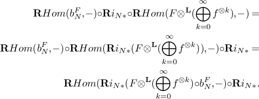 $$ \begin{align*} \mathbf{R}Hom(b_{N}^{F},-){\circ}\mathbf{R}i_{N*}{\circ}\mathbf{R}Hom(F{\otimes}^{\mathbf{L}}(\bigoplus_{k=0}^{\infty}f^{{\otimes}k}),-)=\\ \mathbf{R}Hom(b_{N}^{F},-){\circ}\mathbf{R}Hom(\mathbf{R}i_{N*}(F{\otimes}^{\mathbf{L}}(\bigoplus_{k=0}^{\infty}f^{{\otimes}k})),-){\circ}\mathbf{R}i_{N*}=\\ \mathbf{R}Hom(\mathbf{R}i_{N*}(F{\otimes}^{\mathbf{L}}(\bigoplus_{k=0}^{\infty}f^{{\otimes}k}){\circ}b_{N}^{F},-){\circ}\mathbf{R}i_{N*}. \end{align*} $$
Hence, (C.5) follows from the identity that
 $$ \begin{align*}\mathbf{R}i_{N*}(F{\otimes}^{\mathbf{L}}(\bigoplus_{k=0}^{\infty}f^{{\otimes}k}){\circ}b_{N}^{F}=\mathbf{R}i_{N,M*}(b_{M}^{F}){\circ}\iota_{M,N}^{F}.\\[-47pt]\end{align*} $$
Combining Lemmas C.3 and C.4, we have
Corollary C.5. Let $f:X\to Y$
be a projective morphism of varieties. Let M and N be locally free sheaves on X and Y, respectively, with a surjective morphism
$f:X\to Y$
be a projective morphism of varieties. Let M and N be locally free sheaves on X and Y, respectively, with a surjective morphism $g:f^{*}N\to M$
. The morphism g induces a canonical morphism
$g:f^{*}N\to M$
. The morphism g induces a canonical morphism $g_{N,M}:X_{M}\to Y_{N}$
. Then for any elements
$g_{N,M}:X_{M}\to Y_{N}$
. Then for any elements $F,G\in D^{u}(X)$
, we have the following commutative diagram:
$F,G\in D^{u}(X)$
, we have the following commutative diagram:

C.3 The Bass-Quillen classes and the HKR isomorphism
The Bass-Quillen class comes from the Bass-Quillen conjecture, which asks the following question: let M be a locally free sheaf on X and V be a locally free sheaf on $Tot_{X}(M^{\vee })$
. When is V the pullback of a locally free sheaf on X? While this question is always true if X is affine, an obstruction class would appear when X is not an affine variety.
$Tot_{X}(M^{\vee })$
. When is V the pullback of a locally free sheaf on X? While this question is always true if X is affine, an obstruction class would appear when X is not an affine variety.
In this subsection, we consider a similar but easier question: given a locally free sheaf V on X, classify all the locally free sheaves L on $X_{M}$
, such that
$X_{M}$
, such that $i_{M*}L\cong V$
.
$i_{M*}L\cong V$
.
Theorem C.6. The locally free sheaves L on $X_{M}$
, such that
$X_{M}$
, such that $i_{M}^{*}L\cong V$
are in one-to-one correspondence with elements in
$i_{M}^{*}L\cong V$
are in one-to-one correspondence with elements in $Ext^{1}_{X}(V,V{\otimes }M)$
.
$Ext^{1}_{X}(V,V{\otimes }M)$
.
Proof. An extension class $h\in Ext^{1}_{X}(V,V{\otimes }M)$
induces a short exact sequence:
$h\in Ext^{1}_{X}(V,V{\otimes }M)$
induces a short exact sequence:
 $$ \begin{align} 0\to V{\otimes}M\xrightarrow{\alpha_{h}} L_{0}\xrightarrow{\beta_{h}} V\to 0. \end{align} $$
We define $d_{L}:L_{0}{\otimes }M\to L_{0}$
as
$d_{L}:L_{0}{\otimes }M\to L_{0}$
as ${\alpha }_{h}{\circ }(\beta _{h}{\otimes }M)$
. Then
${\alpha }_{h}{\circ }(\beta _{h}{\otimes }M)$
. Then $d_{L}{\circ }(d_{L}{\otimes }M)=0$
and, hence,
$d_{L}{\circ }(d_{L}{\otimes }M)=0$
and, hence, $L:=(L_{0},d_{L})$
is also locally free on
$L:=(L_{0},d_{L})$
is also locally free on $X_{M}$
.
$X_{M}$
.
On the other hand, given L on $X_{M}$
, such that
$X_{M}$
, such that $i_{M*}L\cong V$
, we have a short exact sequence:
$i_{M*}L\cong V$
, we have a short exact sequence:
 $$ \begin{align} 0\to i_{M*}(V{\otimes}M)\xrightarrow{\alpha_{h}'} L\xrightarrow{\beta_{h}'} i_{M*}V\to 0 \end{align} $$
and, hence, a short exact sequence
 $$ \begin{align*} 0\to V\otimes M\to j_{M*}L\to V\to 0 \end{align*} $$
which induces the extension class $h\in Ext^{1}_{X}(V,V{\otimes }M)$
.
$h\in Ext^{1}_{X}(V,V{\otimes }M)$
.
We say that the extension class $h\in Ext^{1}_{X}(V,V{\otimes }M)$
is the Bass-Quillen class of L, following the notation of [Reference Huang13]. Let M be a locally free sheaf on X. The short exact sequence (C.8) induces an extension class
$h\in Ext^{1}_{X}(V,V{\otimes }M)$
is the Bass-Quillen class of L, following the notation of [Reference Huang13]. Let M be a locally free sheaf on X. The short exact sequence (C.8) induces an extension class $h'\in Ext^{1}_{X_{M}}(i_{M*}V,i_{M*}(V{\otimes }M))$
.
$h'\in Ext^{1}_{X_{M}}(i_{M*}V,i_{M*}(V{\otimes }M))$
.
Lemma C.7. The image of $h'$
under the isomorphism
$h'$
under the isomorphism
 $$ \begin{align*}t_{M}^{V{\otimes}M,V}:Ext^{1}_{X_{M}}(i_{M*}V,i_{M*}(V{\otimes}M)){\cong}Hom_{X}(V,V){\oplus}Ext_{X}^{1}(V,V{\otimes}M)\end{align*} $$
is $(id,h)$
.
$(id,h)$
.
Proof. We recall the description of $Coh(X_{M})$
in the term of (C.1). We denote
$Coh(X_{M})$
in the term of (C.1). We denote $L=(L_{0},d_{L})$
as the locally free sheaf on
$L=(L_{0},d_{L})$
as the locally free sheaf on $X_{M}$
generated by the extension class h. The morphism
$X_{M}$
generated by the extension class h. The morphism $(t_{M}^{V{\otimes }M,V})^{-1}(id,h)$
is induced by the composition of following morphisms of complexes (up to the inverse of quasi-isomorphisms)
$(t_{M}^{V{\otimes }M,V})^{-1}(id,h)$
is induced by the composition of following morphisms of complexes (up to the inverse of quasi-isomorphisms)

and the quasi-isomorphism

We consider the morphism $d:(V{\oplus }L_{0}){\otimes }M\to V{\oplus }L_{0}$
by the matrix
$d:(V{\oplus }L_{0}){\otimes }M\to V{\oplus }L_{0}$
by the matrix
 $$ \begin{align*} \begin{pmatrix} 0 & \alpha_{h} \\ 0 & 0 \end{pmatrix} ,\end{align*} $$
which makes $(V{\oplus }L_{0},d)$
a coherent sheaf on
$(V{\oplus }L_{0},d)$
a coherent sheaf on $X_{M}$
. We consider the following morphism of complexes (up to the inverse of quasi-isomorphisms):
$X_{M}$
. We consider the following morphism of complexes (up to the inverse of quasi-isomorphisms):

We recall the definition of morphism spaces in $D^{u}(X_{M})$
by [34, Tag 04VB] and [34, Tag 05RN] and see that the diagrams in (C.9) and (C.10) represent the same morphism, as their compositions are in the same homotopy class. On the other hand, the morphism
$D^{u}(X_{M})$
by [34, Tag 04VB] and [34, Tag 05RN] and see that the diagrams in (C.9) and (C.10) represent the same morphism, as their compositions are in the same homotopy class. On the other hand, the morphism $h'$
is induced by the following morphism of complexes (up to inverse of quasi-isomorphisms)
$h'$
is induced by the following morphism of complexes (up to inverse of quasi-isomorphisms)

Hence, the equality of $h'$
and
$h'$
and $(t_{M}^{V{\otimes }M,V})^{-1}(id,h)$
follows from the following quasi-isomorphism
$(t_{M}^{V{\otimes }M,V})^{-1}(id,h)$
follows from the following quasi-isomorphism

C.4 The splitting of the first order neighborhood
Let $f:X\to Y$
be a closed embedding of smooth varieties, and let
$f:X\to Y$
be a closed embedding of smooth varieties, and let $N_{Y/X}$
be the normal bundle of X in Y. On X, we have the short exact sequence:
$N_{Y/X}$
be the normal bundle of X in Y. On X, we have the short exact sequence:
 $$ \begin{align*} 0\to N_{Y/X}^{{\vee}}\xrightarrow{\iota_{Y/X}} \Omega_{Y}|_{X}\to \Omega_{X}\to 0. \end{align*} $$
By Lemma C.2, the space
 $$ \begin{align} \{g\in Hom(X_{N_{Y/X}^{{\vee}}},Y)|g{\circ}i_{N_{Y/X}^{{\vee}}}=f\}=Hom_{X}(\Omega_{Y}|_{X},N_{Y/X}^{{\vee}}). \end{align} $$
Let $\mathcal {I}_{X}$
be the ideal sheaf of X in Y and
$\mathcal {I}_{X}$
be the ideal sheaf of X in Y and $X_{(1)}^{Y}:=Spec_{Y}({\mathcal {O}}_{Y}/\mathcal {I}_{X}^{2})$
be the first order infinitesimal neighborhood of X in Y.
$X_{(1)}^{Y}:=Spec_{Y}({\mathcal {O}}_{Y}/\mathcal {I}_{X}^{2})$
be the first order infinitesimal neighborhood of X in Y.
Lemma C.8. Every $g\in Hom_{X}(\Omega _{Y}|_{X},N_{Y/X}^{{\vee }})$
, regarding as a homomorphism from
$g\in Hom_{X}(\Omega _{Y}|_{X},N_{Y/X}^{{\vee }})$
, regarding as a homomorphism from $X_{N_{Y/X}^{{\vee }}}$
to Y, factors through a homomorphism in
$X_{N_{Y/X}^{{\vee }}}$
to Y, factors through a homomorphism in $Hom(X_{N_{Y/X}^{{\vee }}},X_{(1)}^{Y})$
. Moreover, g induces an isomorphism between
$Hom(X_{N_{Y/X}^{{\vee }}},X_{(1)}^{Y})$
. Moreover, g induces an isomorphism between $X_{N_{Y/X}^{{\vee }}}$
and
$X_{N_{Y/X}^{{\vee }}}$
and $X_{(1)}^{Y}$
if and only if
$X_{(1)}^{Y}$
if and only if $g{\circ }\iota _{Y/X}$
is an isomorphism of
$g{\circ }\iota _{Y/X}$
is an isomorphism of $N_{Y/X}^{{\vee }}$
.
$N_{Y/X}^{{\vee }}$
.
Proof. The morphism g induces a homomorphism of ${\mathcal {O}}_{Y}$
-algebras
${\mathcal {O}}_{Y}$
-algebras $g^{\#}=(f^{\#},h^{\#}):{\mathcal {O}}_{Y}\to {\mathcal {O}}_{X}{\oplus }N_{Y/X}^{{\vee }}$
, where
$g^{\#}=(f^{\#},h^{\#}):{\mathcal {O}}_{Y}\to {\mathcal {O}}_{X}{\oplus }N_{Y/X}^{{\vee }}$
, where $f^{\#}$
is the quotient morphism and
$f^{\#}$
is the quotient morphism and $h^{\#}$
is the derivative induced by g. As
$h^{\#}$
is the derivative induced by g. As ${\mathcal {I}}_{X}$
is the kernel of
${\mathcal {I}}_{X}$
is the kernel of $f^{\#}$
, the image of
$f^{\#}$
, the image of ${\mathcal {I}}_{X}^{2}$
in
${\mathcal {I}}_{X}^{2}$
in $g^{\#}$
is
$g^{\#}$
is $0$
and, hence, induces a homomorphism in
$0$
and, hence, induces a homomorphism in $Hom(X_{N_{Y/X}^{{\vee }}},X_{(1)}^{Y})$
. Moreover, we have the short exact sequence of
$Hom(X_{N_{Y/X}^{{\vee }}},X_{(1)}^{Y})$
. Moreover, we have the short exact sequence of ${\mathcal {O}}_{Y}$
modules:
${\mathcal {O}}_{Y}$
modules:

Hence, $g^{\#}$
induces an isomorphism between
$g^{\#}$
induces an isomorphism between ${\mathcal {O}}_{Y}/{\mathcal {I}}_{X}^{2}$
and
${\mathcal {O}}_{Y}/{\mathcal {I}}_{X}^{2}$
and ${\mathcal {O}}_{X}{\oplus }N_{Y/X}^{{\vee }}$
if and only if
${\mathcal {O}}_{X}{\oplus }N_{Y/X}^{{\vee }}$
if and only if $g{\circ }\iota _{Y/X}$
is an isomorphism.
$g{\circ }\iota _{Y/X}$
is an isomorphism.
Lemma C.8 could be generalised to a relative version. We consider a Cartesian diagram of smooth varieties: Let $f':X\to Y$
be a regular embedding of smooth varieties. Let
$f':X\to Y$
be a regular embedding of smooth varieties. Let $\pi :Y'\to Y$
be a proper morphism of smooth varieties. Let
$\pi :Y'\to Y$
be a proper morphism of smooth varieties. Let $X'=Y'\times _{Y}X$
and
$X'=Y'\times _{Y}X$
and $f:X'\to Y'$
and
$f:X'\to Y'$
and $\pi _{X}:X'\to X$
be the respective fibre morphisms. Moreover, we assume that
$\pi _{X}:X'\to X$
be the respective fibre morphisms. Moreover, we assume that $X'$
is also smooth.
$X'$
is also smooth.
Lemma C.9. There exists a canonical morphism of short exact sequences:

where the middle and right rows are the canonical morphisms of differentials. Moreover, a splitting of $\iota _{Y'/X'}$
and
$\iota _{Y'/X'}$
and $\iota _{Y/X}$
, which is compatible with (C.13), which we denote as
$\iota _{Y/X}$
, which is compatible with (C.13), which we denote as $g'$
and g, respectively, would induce a commutative diagram
$g'$
and g, respectively, would induce a commutative diagram

where $g'$
and g are isomorphisms.
$g'$
and g are isomorphisms.
Finally, we explain the relation between the isomorphism $t_{M}^{F,G}$
and the HKR isomorphism. Given a locally free sheaf M on a scheme X and a positive integer k, there is a canonical shuffle morphism
$t_{M}^{F,G}$
and the HKR isomorphism. Given a locally free sheaf M on a scheme X and a positive integer k, there is a canonical shuffle morphism
 $$ \begin{align*} sh_{k}:M^{{\otimes}k}&\to {\wedge}^{k}(M) \\ v_{1}{\otimes}{\cdots}{\otimes}v_{k}&\to v_{1}{\wedge}{\cdots}{\wedge}v_{k}. \end{align*} $$
Given a regular embedding of smooth varieties $f:X\to Y$
, we denote
$f:X\to Y$
, we denote $M=N_{Y/X}^{{\vee }}$
. We fix a splitting
$M=N_{Y/X}^{{\vee }}$
. We fix a splitting $g\in Hom_{X}(\Omega _{Y}|_{X},N_{Y/X}^{{\vee }})$
, such that
$g\in Hom_{X}(\Omega _{Y}|_{X},N_{Y/X}^{{\vee }})$
, such that $g{\circ }\iota _{Y/X}=id$
and abuse the notation to denote g as the closed embedding from
$g{\circ }\iota _{Y/X}=id$
and abuse the notation to denote g as the closed embedding from $X_M$
to Y.
$X_M$
to Y.
Theorem C.10 (HKR isomorphism, Theorem 1.4 and Section 1.11 of [Reference Arinkin and Căldăraru1]).
Let $\tau _{M}^{F,G}$
be the composition of the following morphisms:
$\tau _{M}^{F,G}$
be the composition of the following morphisms:
 $$ \begin{align*} \mathbf{R}Hom_{X}(F{\otimes}^{\mathbf{L}}\bigoplus_{k=0}^{\infty}{\wedge}^{k}M[k],G)&\xrightarrow{\mathbf{R}Hom_{X}(F{\otimes}^{\mathbf{L}}sh_{k},-)}\mathbf{R}Hom_{X}(F{\otimes}^{\mathbf{L}}\bigoplus_{k=0}^{\infty}M^{{\otimes}k}[k],G)\\ & \xrightarrow{t_{M}^{F,G}} \mathbf{R}Hom_{X_{M}}(\mathbf{R}i_{M*}F,\mathbf{R}i_{M*}G) \\ & \xrightarrow{\mathbf{R}g_{*}} \mathbf{R}Hom_{Y}(\mathbf{R}f_{*}F,\mathbf{R}f_{*}G). \end{align*} $$
Then $\tau _{M}^{F,G}$
is an isomorphism.
$\tau _{M}^{F,G}$
is an isomorphism.
Now we combine Lemmas C.7 and C.9 and Theorem C.10 to induce an extension formula. We recall the schemes of $X,Y,X',Y'$
and morphisms in the setting of Lemma C.9 and assume that
$X,Y,X',Y'$
and morphisms in the setting of Lemma C.9 and assume that $s_{f,\pi }$
in (C.13) is surjective. We fix splittings
$s_{f,\pi }$
in (C.13) is surjective. We fix splittings $g'$
and g in Lemma C.9. Let L be a locally free sheaf on
$g'$
and g in Lemma C.9. Let L be a locally free sheaf on ${X'}_{(1)}^{Y'}$
and
${X'}_{(1)}^{Y'}$
and $V:=L|_{X'}$
. Then L induces extension classes
$V:=L|_{X'}$
. Then L induces extension classes $h_{L}'\in Ext_{X'}^{1}(V, V{\otimes }M)$
and
$h_{L}'\in Ext_{X'}^{1}(V, V{\otimes }M)$
and $h_{L}\in Ext_{Y'}^{1}(f^{\prime }_{*}V,f^{\prime }_{*}V{\otimes }M)$
, such that
$h_{L}\in Ext_{Y'}^{1}(f^{\prime }_{*}V,f^{\prime }_{*}V{\otimes }M)$
, such that $h_{L}$
induces the short exact sequence:
$h_{L}$
induces the short exact sequence:
 $$ \begin{align} 0\to f^{\prime}_{*}V{\otimes}M\to L\to f^{\prime}_{*}V\to 0 ,\end{align} $$
where we abuse the notation to denote L as a coherent sheaf on $Y'$
through the pushforward of the closed embedding
$Y'$
through the pushforward of the closed embedding ${X'}_{(1)}^{Y'}\to Y'$
. By applying then functor
${X'}_{(1)}^{Y'}\to Y'$
. By applying then functor $\mathbf {R}\pi _{*}$
to (C.15), we induce a triangle:
$\mathbf {R}\pi _{*}$
to (C.15), we induce a triangle:
 $$ \begin{align*}{\cdots}\to \mathbf{R}\pi_{*}(f^{\prime}_{*}V{\otimes}M)\to \mathbf{R}\pi_{*}L\to \mathbf{R}\pi_{*}(f^{\prime}_{*}V)\to \mathbf{R}\pi_{*}(f^{\prime}_{*}V{\otimes}M)[1]\to {\cdots}\end{align*} $$
and thus induce an extension class
 $$ \begin{align*}e_{L}=\mathbf{R}\pi_{*}h_{L}\in \mathbf{R}Hom_{Y}(\mathbf{R}\pi_{*}(f^{\prime}_{*}V),\mathbf{R}\pi_{*}(f^{\prime}_{*}V{\otimes}M)[1]).\end{align*} $$
Theorem C.11. The image of $e_{L}$
under the HKR isomorphism in Theorem C.10 is
$e_{L}$
under the HKR isomorphism in Theorem C.10 is
 $$ \begin{align*}(\mathbf{R}\pi_{X*}h_{L},\mathbf{R}\pi_{X*}(V{\otimes}s_{f,\pi}),0,{\cdots},0).\end{align*} $$
Remark C.12. One should notice that while the Bass-Quillen class $h_{L}$
depends on L,
$h_{L}$
depends on L, $\mathbf {R}\pi _{X*}(V{\otimes }s_{f,\pi })$
only depends on V but not the line bundle L.
$\mathbf {R}\pi _{X*}(V{\otimes }s_{f,\pi })$
only depends on V but not the line bundle L.
Acknowledgments
The author would like to acknowledge Andrei Neguts and Lucas Mason-Brown for their continued support, academically and spiritually. The author is grateful to Jihao Liu and Ziquan Zhuang for their help in understanding the minimal model program and Yuchen Liu for checking the Appendix B. The author would like to thank Qingyuan Jiang, Huachen Chen, Xiaolei Zhao, Shizhuo Zhang, Andreas Krug and Sabin Cautis for many interesting discussions on the subject. Special thanks to Kai Xu and Shengyuan Huang for explaining the functionality of the HKR isomorphism. The author would also like to thank the anonymous referee for many useful suggestions. The author is partly supported by the National Science Foundation (NSF) Career grant Division of Mathematical Sciences (DMS)-1845034, World Premier International Research Center Initiative (WPI initiative), Ministry of Education, Culture, Sports, Science and Technology (MEXT), Japan and Japan Society for the Promotion of Science (JSPS) Grants-in-Aid for Scientific Research (KAKENHI) Number 22K13889.
Competing Interests
None.


 Open access