


1 Introduction
There has been considerable research on the subject of the dynamics of a supersonic microjet for the application of microscale devices, including a small satellite thruster in space engineering (Bayt & Breuer Reference Bayt and Breuer2001; Lempert et al. Reference Lempert, Boehm, Jiang, Gimelshein and Levin2003), a critical nozzle for obtaining mass flow rate at a low Reynolds number (Nakao & Takamoto Reference Nakao and Takamoto2000), and a micro-propulsion nozzle (Louisos & Hitt Reference Louisos and Hitt2007). A detailed knowledge of the flow characteristics through such devices requires information regarding the quantitative velocity, density and temperature measurements in the flow field. Until recently, however, there has been very little experimental data on supersonic microjets available in the literature. To the best of our knowledge, the definition of microjets is ambiguous and still controversial in the literature (Scroggs & Settles Reference Scroggs and Settles1996; Phalnikar, Kumar & Alvi Reference Phalnikar, Kumar and Alvi2008; Mironov et al. Reference Mironov, Aniskin, Korotaeva and Tsyryulnikov2019). However, in the present study, a microjet is defined as a free jet discharged from an orifice or a nozzle with a diameter or height smaller than approximately 1 mm. It should be noted that Mironov et al. (Reference Mironov, Aniskin, Korotaeva and Tsyryulnikov2019) defined microjets as those escaping from nozzles with a diameter that is smaller than  $200~\unicode[STIX]{x03BC}\text{m}$ (for the case of axisymmetric nozzles).
The structure of supersonic microjets was systematically studied for the first time by Scroggs & Settles (Reference Scroggs and Settles1996), who made axisymmetric nozzles with exit Mach numbers ranging from 1.0 to 2.8 and two different inner diameters of  $600~\unicode[STIX]{x03BC}\text{m}$ and $1200~\unicode[STIX]{x03BC}\text{m}$ at the nozzle exit. They measured the Pitot pressures along the jet centreline by impinging the jet upon a flat plate, including a pressure port of 0.2 mm in diameter with a pressure sensor attached to the reverse side. Phalnikar et al. (Reference Phalnikar, Kumar and Alvi2008) fabricated a micro Pitot probe with a pressure hole of $50~\unicode[STIX]{x03BC}\text{m}$ in diameter, and later Aniskin, Mironov & Maslov (Reference Aniskin, Mironov and Maslov2013) developed one with an intake port of $12~\unicode[STIX]{x03BC}\text{m}$ diameter. These two research groups performed Pitot pressure measurements to study the size of shock-cells and the supersonic core length of the microjet. The intrusive probe, including a Pitot probe, a static pressure tube and a hot-wire anemometer, can only measure the flow parameters at discrete points. Such probes are also very sensitive to the flow alignment (John Reference John1984). In addition, the intrusive probe can alter the flow fields since the presence of the probe located inside the flow can change the shock structures significantly. Recently, Mironov et al. (Reference Mironov, Aniskin, Korotaeva and Tsyryulnikov2019) investigated the influence of the Pitot tube diameter on the axial pressure distribution and the supersonic core length in an underexpanded microjet. The study demonstrated that the Pitot pressure distribution along the centreline of the microjet is shifted in the downstream direction with respect to the curves that are calculated for free microjets. (Note that detached shock waves are formed on the Pitot tube.)
Non-intrusive techniques such as the laser Doppler and particle image velocimetry can be used for velocity measurements. However, these techniques often contain an inherent error because the tracer particles cannot necessarily follow a strong velocity gradient across a shock wave (Koike et al. Reference Koike, Suzuki, Kitamura, Hirota, Takita, Masuya and Matsumoto2006; Huffman & Elliott Reference Huffman and Elliott2009; Sakurai et al. Reference Sakurai, Handa, Koike, Mii and Nakano2015; Wernet Reference Wernet2016). Therefore, with complex shock-containing structures, a proper and homogeneous seeding is very difficult. For an update on particle response analysis for particle image velocimetry in supersonic and hypersonic flows, Williams et al. (Reference Williams, Nguyen, Schreyer and Smits2015) showed that it is necessary to solve the unsteady drag equation. Their model takes into account inertial, compressibility and slip effects in order to obtain an accurate estimate of the particle response (note that the frequency response of particles used for flow velocimetry could be strongly affected by deviations from the Stokes drag). Another class of optical techniques includes a coherent anti-Stokes Raman scattering (Woodmansee et al. Reference Woodmansee, Iyer, Dutton and Lucht2004) to measure pressure and temperature fields and a filtered Rayleigh scattering (Forkey, Lempert & Miles Reference Forkey, Lempert and Miles1998; Panda & Seasholtz Reference Panda and Seasholtz1999; Gustavsson & Segal Reference Gustavsson and Segal2005) to measure velocity fields. A detailed review on the laser scattering technique can be found in the paper of Miles, Lempert & Forkey (Reference Miles, Lempert and Forkey2001).
For a supersonic free jet operating at slightly off-design conditions, several analytical models predicting the flow properties inside a jet plume have been proposed (Pack Reference Pack1950; Tam Reference Tam1972, Reference Tam1988; Tam, Jackson & Seiner Reference Tam, Jackson and Seiner1985; Morris, Bhat & Chen Reference Morris, Bhat and Chen1989; Emami, Bussmann & Tran Reference Emami, Bussmann and Tran2009). However, no exact solutions exist for a supersonic free jet with strong shock waves such as Mach disks and barrel shocks, or with shock wave–vortex interactions.
As a computational fluid dynamics (CFD) analytical tool, Reynolds-averaged Navier–Stokes (RANS) simulations have been used to provide reasonably accurate results within a relatively short period of computational time (Chin et al. Reference Chin, Li, Harkin, Rochwerger, Chan, Ooi, Risborg and Soria2013; Franquet et al. Reference Franquet, Perrier, Gibout and Bruel2015). Although the RANS models have been applied to various engineering applications, exact solutions cannot be obtained due to the fact that these numerical models are not ‘closed’. The RANS models rely on additional physical approximations (for instance, a turbulence model needs a closure model for the Reynolds stress with the help of model parameters, which need to be adjusted depending on flow characteristics such as Reynolds numbers, etc.). Therefore, it is critical that the capabilities of these models are assessed before the numerical results are accepted. To validate a computational model, reliable experimental datasets are thus very important. A widely used method for the validation of numerical simulations of a microjet is pressure measurement data obtained by use of a Pitot probe (Liu et al. Reference Liu, Kailasanath, Ramamurti, Munday, Gutmark and Lohner2009; Miller et al. Reference Miller, Veltin, Morris and McLaughlin2009; Emami, Bussmann & Tran Reference Emami, Bussmann and Tran2010).
The schlieren and shadowgraph techniques (Settles Reference Settles2001) have been used routinely for qualitative flow visualization, providing quantitative information of geometrical features such as positions, lengths and shapes of shock waves. This information has been used to validate computational models (Loh & Hultgren Reference Loh and Hultgren2006; Li, Yao & Fan Reference Li, Yao and Fan2016; Li et al. Reference Li, Zhou, Yao and Fan2017). However, the validation of simulations by comparisons with the geometrical shapes of shock waves from the schlieren or shadowgraph pictures should be done with care, because the conventional schlieren or shadowgraph image is taken by a line-of-sight imaging technique (i.e. these pictures exhibit information averaged along the view direction about the first or second spatial derivative of density profiles). Results from numerical simulations are typically not obtained in the same way, and thus this validation process might be inconsistent. In contrast, although it used to be very difficult to obtain quantitative information of the density profile in flows by a schlieren technique, the integration and subsequent processing analyses can now be done with ease by conventional personal computers (Settles & Hargather Reference Settles and Hargather2017; Agrawal & Wanstall Reference Agrawal and Wanstall2018). There have been some recent attempts to visualize the prominent characteristics of shock-containing microjets by quantitatively utilizing a computer-based imaging approach. Kolhe & Agrawal (Reference Kolhe and Agrawal2009) applied for the first time the rainbow schlieren deflectometry to a shock-containing jet issued from a micro cylindrical nozzle with an inner diameter of  $500~\unicode[STIX]{x03BC}\text{m}$ at the nozzle exit. Maeda et al. (Reference Maeda, Fukuda, Nakao, Miyazato and Ishino2018) measured the density in a slightly underexpanded free jet issued from a micro nozzle with a design Mach number of 1.5 and a square shape of $1~\text{mm}\times 1~\text{mm}$ at the nozzle exit plane. In their approach, a rainbow schlieren system combined with the computed tomography was utilized to reconstruct the jet three-dimensional density fields. Sugawara et al. (Reference Sugawara, Nakao, Miyazato, Ishino and Rösgen2018) carried out a preliminary experiment to obtain the density field of a shock-containing microjet by the Twyman–Green interferometer system and also performed the RANS simulations with Menter’s (shear stress transport) SST $k$–
$k$– $\unicode[STIX]{x1D714}$ turbulence model. Although a Mach disk exists in the jet plume in the actual flow field, their experimental and numerical approaches failed to capture a Mach disk.
In the present study, an axisymmetric convergent nozzle with an exit diameter  $=1~\text{mm}$ is used as the first step for obtaining three-dimensional density fields of a supersonic microjet that shows complex shock structures. To this aim, the Mach–Zehnder interferometer (Born & Wolf Reference Born and Wolf2011) is utilized to investigate the three-dimensional density fields of a microjet with a Mach disk, which could be useful for the CFD community as validation data against their numerical simulations of shock-containing microjets. In addition, quantitative comparisons among the present experiment and the previous visualization studies for the jet centreline density profiles are performed in order to investigate the effects of the measuring methods on the density profiles and the nozzle dimensions.
2 Experimental apparatus
The experiments were conducted in a blowdown compressed-air facility of the High-Speed Gasdynamics Laboratory at the University of Kitakyushu. A schematic diagram of the experimental apparatus with the laser interferometer system is shown in figure 1. Ambient air is pressurized by the compressor up to 1 MPa, and then stored in the high-pressure reservoir consisting of two storage tanks with a total capacity of  $2~\text{m}^{3}$ after being filtered and dried. The high-pressure dry air from the reservoir is stagnated in a plenum chamber as shown in figure 1, and then discharged into the atmosphere through a test nozzle. In the present experiment, the plenum pressure is controlled and maintained constant at a value of $p_{os}=405\pm 0.5~\text{kPa}$ during testing by a solenoid valve.

Figure 1. Schematic drawing of experimental apparatus.
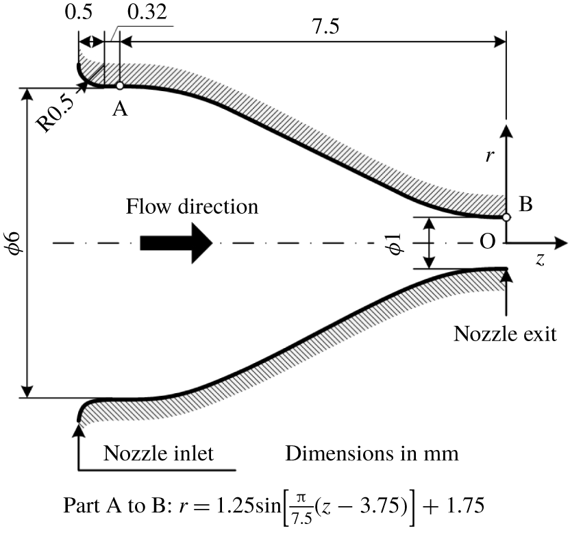
Figure 2. Schematic of the test nozzle.
As schematically shown in figure 2, an axisymmetric convergent nozzle with 6 mm and 1 mm diameter at the inlet and exit was used as a test nozzle. The nozzle wall contour from the inlet to the exit was designed based on a sinusoidal curve so as to realize smooth uniform flows at the inlet and exit. The experiment was carried out at a nozzle pressure ratio (NPR) of 4.0 within an accuracy of  $\pm$1.0 % to produce an underexpanded free jet with a Mach disk. The total temperature in the plenum chamber was equal to the room temperature ( $T_{b}=300~\text{K}$) within an accuracy of approximately $0.1\,^{\circ }\text{C}$ during the experiment. To obtain density fields in a shock-containing microjet, quantitative flow visualization was performed using the Mach–Zehnder interferometer system with a field of view of 50 mm diameter. The Reynolds number at the nozzle exit is $Re_{d}=5.91\times 10^{4}$, which is calculated based on the assumption of an isentropic flow from the nozzle inlet to the exit.
The Mach–Zehnder interferometer is an optical instrument of high precision and versatility (see figure 1) with the associated optical equipment that uses a blue semiconductor laser with a wavelength of 405 nm as a light source. The laser beam is expanded by a spatial filter to make a coherent beam before being collimated into a parallel beam, and then is split into reference and test beams by a beam splitter (BS1). The beam splitter reflects roughly half of the intensity of the wavefront in one direction and transmits the rest in another direction. The reference beam passes through the still air and travels to another beam splitter (BS2) after being reflected at mirror 1. The test beam passes through a refractive-index field produced by a free jet that is issued from a test nozzle and also travels to BS2 after being reflected at mirror 2. The two beams are combined before being focused by the imaging lens and then produce interferograms on the recording medium in a digital camera.
To estimate the error of circularity for the wall shape at the nozzle exit section, we obtained a digital image of the section by the laser scanning microscope (Olympus Model LEXT OLS4100). After reading the image in a personal computer, the radial distances from a certain reference point to the wall periphery were measured at each angle of  $20^{\circ }$ around the reference point with AutoCAD 2013 software. The precision error for the radius $r$ of the least-squares circle becomes $\pm 1.4~\unicode[STIX]{x03BC}\text{m}$ and it corresponds to around $\pm$0.3 % of the radius.
3 Reconstruction of jet density fields
The method for reconstructing a jet density field consists of two steps. The first is acquisition of the values of fringe shifts from their original positions measured in the experiment, which is followed by the calculation of density values using the resulting fringe shifts. The former can be done using the Fourier transform method presented by Takeda, Ina & Kobayashi (Reference Takeda, Ina and Kobayashi1982) and the latter by Nestor & Olsen (Reference Nestor and Olsen1960) for the Abel inversion method under the assumption of an axisymmetric density field. The methodology of extracting the density field using both of the methods is described below.
Generally, Mach–Zehnder interferometers can be arranged so as to produce either finite fringe or infinite fringe patterns. In the infinite fringe method, each fringe occurs due to a one-wavelength shift in the optical path length as a result of changes in the flow field (Smits & Lim Reference Smits and Lim2000). The finite fringe method seems to be more suitable for a quantitative evaluation of the fringes since it is easier to measure fringe distortions (as demonstrated in the present paper) than to identify the values of the density contour lines given by the infinite fringe approach. In addition, in the infinite fringe method, it is necessary to know some information about the flow field when interpreting the results (Smits & Lim Reference Smits and Lim2000) because the sign of the change in the phase shift is ambiguous. In the finite fringe method, the mirrors and the beam splitter are deliberately misaligned to produce an initial fringe pattern or a background fringe pattern of straight lines. The image is then processed using techniques for obtaining density fields by digital subtraction of the background fringe pattern from the deformed fringe pattern. In the present experiment, the background fringes were set in the horizontal orientation with respect to the nozzle axis by the appropriate adjustment of mirror 2 as shown in figure 1.
3.1 Fourier transform method
When the test beam passes through a free jet with a variable refractive-index field, the background fringes are changed into the deformed fringe patterns because of the phase shift caused by the variations of the light speed as the beam passes through the test field. Typical profiles taken using a camera showing background and the deformed fringe patterns are illustrated in figure 3 as lines of constant phase. The parallel and equally spaced fringes shown as blue solid lines in figure 3(a) are also referred to as wedge fringes. The interval  $b$ in figure 3(a) denotes the distance between two successive crests of the background fringes, and it is a function of the intersection angle between the reference and the test beams and the wavelength of the laser light used in the experiment. The red dashed line in figure 3(b) shows the intensity profile $g(y,z_{0})$ corresponding to the deformed fringe pattern at a particular axial position $z_{0}$, and it can be given by (Takeda et al. Reference Takeda, Ina and Kobayashi1982; Yagi et al. Reference Yagi, Inoue, Nakao, Ono and Miyazato2017)
 $$\begin{eqnarray}g(y,z_{0})=g_{0}(y,z_{0})+g_{1}(y,z_{0})\cos [k_{0}y-\unicode[STIX]{x0394}\unicode[STIX]{x1D711}(y,z_{0})].\end{eqnarray}$$
 Here, the phase shift  $\unicode[STIX]{x0394}\unicode[STIX]{x1D711}(y,z_{0})$ contains the desired information on the density field in the free jet, and $g_{0}(y,z_{0})$ and $g_{1}(y,z_{0})$ represent unwanted irradiance variations arising from the non-uniform light reflection or transmission when the test beam passes through a free jet, and $k_{0}=2\unicode[STIX]{x03C0}/b$. The coordinates $y$ and $z$ form the vertical plane, which is perpendicular to the test beam propagation direction, and the $x$-axis is taken as the direction in which the test beam propagates after being reflected at mirror 2, as shown in figure 1.
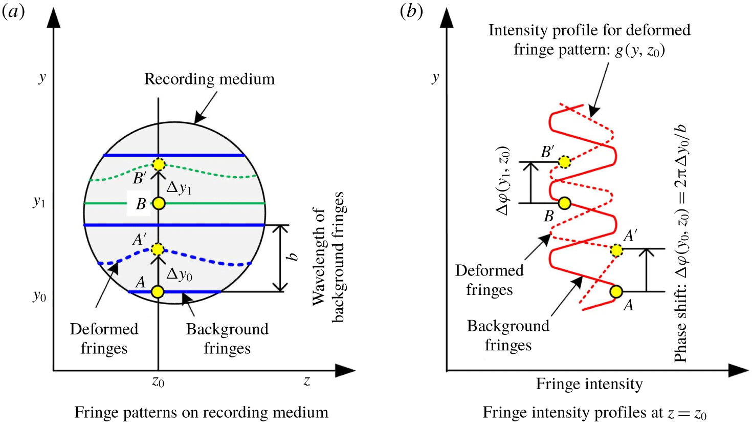
Figure 3. Variation of background and deformed fringes by the finite fringe method.
Equation (3.1) can be rewritten in the following form:
 $$\begin{eqnarray}g(y,z_{0})=g_{0}(y,z_{0})+c(y,z_{0})\exp (\text{i}k_{0}y)+c^{\ast }(y,z_{0})\exp (-\text{i}k_{0}y),\end{eqnarray}$$
with
 $$\begin{eqnarray}c(y,z_{0})={\textstyle \frac{1}{2}}g_{1}(y,z_{0})\exp [-\text{i}\unicode[STIX]{x0394}\unicode[STIX]{x1D711}(y,z_{0})],\end{eqnarray}$$
 where  $\text{i}$ is the imaginary unit and the asterisk $^{\ast }$ denotes the complex conjugate.
The Fourier transform of (3.2) with respect to  $y$ is given by
 $$\begin{eqnarray}G(k,z_{0})=G_{0}(k,z_{0})+C(k-k_{0},z_{0})+C^{\ast }(k+k_{0},z_{0}),\end{eqnarray}$$
 where the capital letters denote the Fourier transforms of the respective primitive functions, and  $k$ is the spatial wavenumber in the $y$ direction. Since the spatial variations of $g_{0}(y,z_{0})$, $g_{1}(y,z_{0})$ and $\unicode[STIX]{x0394}\unicode[STIX]{x1D711}(y,z_{0})$ are slow compared with the spatial frequency $k_{0}$ when the interval between fringes is sufficiently small, the Fourier spectra in (3.4) are separated by the wavenumber $k_{0}$ and have the three independent peaks as schematically shown in figure 4(a). We make use of either of these two spectra on the carrier, say $C(k-k_{0},z_{0})$, and translate it by $k_{0}$ on the wavenumber axis towards the origin to obtain $C(k,z_{0})$ as shown in figure 4(b). The unwanted background variation $G_{0}(k,z_{0})$ has been filtered out at this stage by the pertinent bandpass filter.
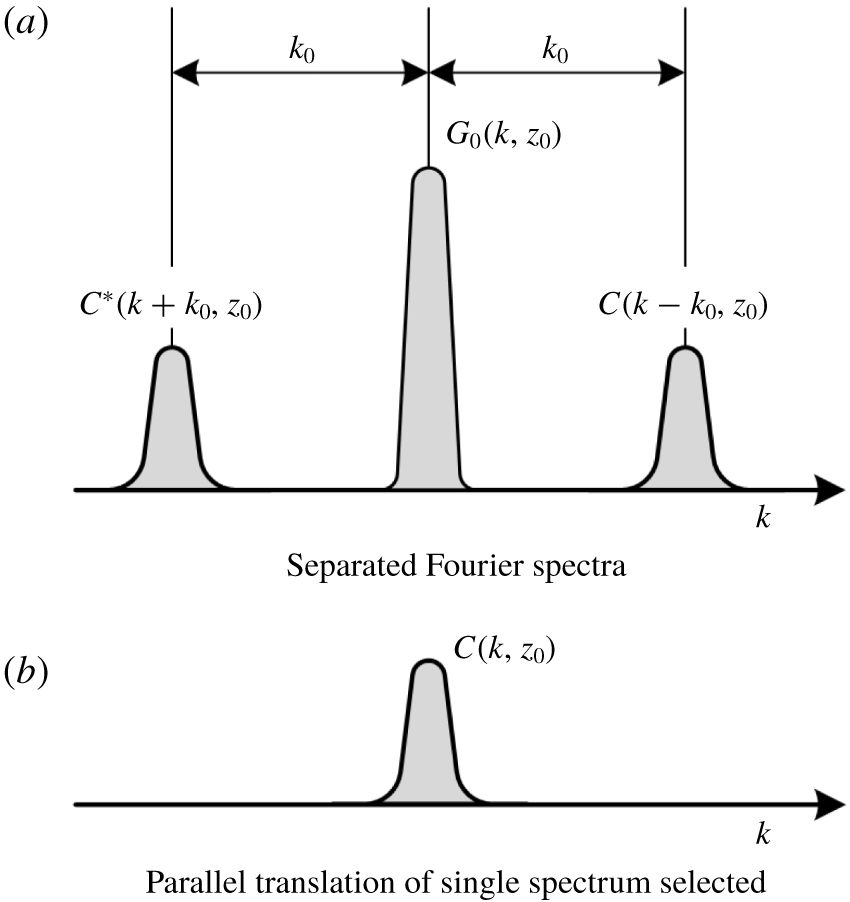
Figure 4. Fourier transform method for fringe-pattern analysis.
Applying the inverse Fourier transform of  $C(k,z_{0})$ with respect to $k$ to obtain $c(y,z_{0})$ defined by (3.3) and taking the logarithm of (3.3) leads to
 $$\begin{eqnarray}\ln c(y,z_{0})=\ln \frac{g_{1}(y,z_{0})}{2}-\text{i}\unicode[STIX]{x0394}\unicode[STIX]{x1D711}(y,z_{0}).\end{eqnarray}$$
 Consequently, the phase shift  $\unicode[STIX]{x0394}\unicode[STIX]{x1D711}(y,z_{0})$ in the imaginary part of (3.5) can be completely separated from the unwanted amplitude variation $g_{1}(y,z_{0})$ in the real part. It is necessary to make the interval $b$ between parallel fringes as narrow as possible to avoid islands in the fringe pattern. Wide fringes move farther away from the original location than narrower fringes, and, as a result, they cover regions that are considerably different from the optical retardations. This results in the creation of islands (Winckler Reference Winckler1948).
3.2 Abel inversion method
A free jet with an axisymmetric refractive-index field is depicted in figure 5(a). The refractive index  $n$ in the flow field depends only on the radial distance $r$ from the centreline O ( $x=y=0$) for a fixed axial distance $z_{0}$ measured from the nozzle exit plane, i.e.
 $$\begin{eqnarray}n=n(r,z_{0}),\quad \text{for }0\leqq r\leqq R,\quad n=n_{a},\quad \text{for }R<r,\end{eqnarray}$$
 where  $n_{a}$ is the refractive index for the ambient air and $R$ is the radial distance to the jet boundary.
Refractive-index values can be obtained directly from the measured fringe positions on a given cross-section normal to the jet axis, and each measured cross-section is independent of others. As illustrated in figure 5(a), the optical path difference  $\unicode[STIX]{x1D6EC}(y,z_{0})$ of the test beam that passes through the field with and without the jet can be expressed by
 $$\begin{eqnarray}\unicode[STIX]{x1D6EC}(y,z_{0})=2\int _{y}^{R}\frac{[n(r,z_{0})-n_{a}]}{\sqrt{r^{2}-y^{2}}}r\,\text{d}r.\end{eqnarray}$$
 The fringe shift  $\unicode[STIX]{x0394}y$ at any location on a recording medium can be related to $\unicode[STIX]{x1D6EC}(y,z_{0})$ as follows:
 $$\begin{eqnarray}\unicode[STIX]{x0394}y=\frac{b}{\unicode[STIX]{x1D706}_{0}}\unicode[STIX]{x1D6EC}(y,z_{0}),\end{eqnarray}$$
 where  $\unicode[STIX]{x1D706}_{0}$ is the wavelength of light in vacuum for the laser used. The use of the Gladstone–Dale relation
 $$\begin{eqnarray}n(r,z)=1+K\unicode[STIX]{x1D70C}(r,z)\end{eqnarray}$$
with the combination of (3.7) and (3.8) gives
 $$\begin{eqnarray}\unicode[STIX]{x0394}y=\frac{2bK}{\unicode[STIX]{x1D706}_{0}}\int _{y}^{R}\frac{[\unicode[STIX]{x1D70C}(r,z_{0})-\unicode[STIX]{x1D70C}_{a}]}{\sqrt{r^{2}-y^{2}}}r\,\text{d}r,\end{eqnarray}$$
 where  $K$ is the Gladstone–Dale constant and $\unicode[STIX]{x1D70C}_{a}$ is the density of ambient air.
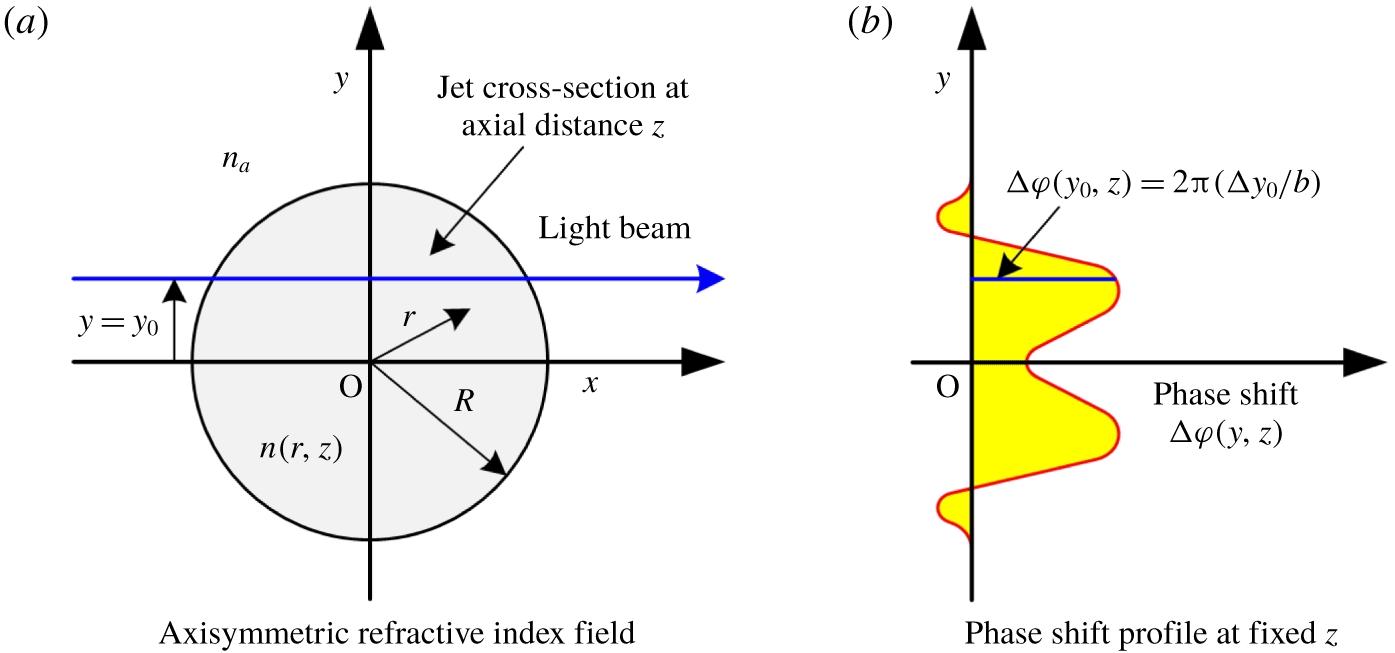
Figure 5. Light beam passing through axisymmetric refractive-index field.
Once the fringe shifts for a fixed streamwise location  $z_{0}$ are obtained by the Fourier transform method, the density field is found by inverting (3.10) using the Abel inversion (Sneddon Reference Sneddon1972):
 $$\begin{eqnarray}\unicode[STIX]{x1D70C}(r,z_{0})=\unicode[STIX]{x1D70C}_{a}-\frac{\unicode[STIX]{x1D706}_{0}}{\unicode[STIX]{x03C0}bK}\int _{r}^{R}\frac{1}{\sqrt{y^{2}-r^{2}}}\frac{\text{d}}{\text{d}y}(\unicode[STIX]{x0394}y)\,\text{d}y.\end{eqnarray}$$
Measurements of the fringe shifts only provide a discrete set of values, and therefore (3.11) can only be solved numerically. Several algorithms for solving the Abel inversion equation have been proposed so far (Nestor & Olsen Reference Nestor and Olsen1960; Bradley Reference Bradley1968; Behjat, Tallents & Neely Reference Behjat, Tallents and Neely1997; Malka et al. Reference Malka, Coulaud, Geindre, Lopez, Najmudin, Neely and Amiranoff2000; Álvarez, Rodero & Quintero Reference Álvarez, Rodero and Quintero2002; Shimomiya, Ono & Miyazato Reference Shimomiya, Ono and Miyazato2013). Among them, the integral in (3.11) is evaluated by using the algorithm proposed by Nestor & Olsen (Reference Nestor and Olsen1960) as follows:
 $$\begin{eqnarray}\unicode[STIX]{x1D70C}(r_{k},z_{0})=\unicode[STIX]{x1D70C}_{a}-\frac{\unicode[STIX]{x1D706}_{0}}{\unicode[STIX]{x03C0}^{2}K\unicode[STIX]{x0394}w}\mathop{\sum }_{n=k}^{N}B_{k,n}\unicode[STIX]{x0394}\unicode[STIX]{x1D711}(y_{n},z_{0}),\end{eqnarray}$$
 where  $r_{k}=k\unicode[STIX]{x0394}w$ ( $k=0,1,2,\ldots ,N$) is the radial distance from the jet centreline, $\unicode[STIX]{x0394}w$ is the sampling interval, which is the same as the distance between neighbouring pixels on the recording medium, $N$ is the total number of intervals in the medium, $\unicode[STIX]{x0394}\unicode[STIX]{x1D711}(y_{n},z_{0})=2\unicode[STIX]{x03C0}y_{n}/b$, $y_{n}\leqq y<y_{n+1},$ $y_{n}=n\unicode[STIX]{x0394}w$ and
 $$\begin{eqnarray}B_{k,n}=-A_{k,n}\quad \text{if }n=k,\quad B_{k,n}=A_{k,n-1}-A_{k,n}\quad \text{if }n\geqq k+1,\end{eqnarray}$$
with
 $$\begin{eqnarray}A_{k,n}=\frac{\sqrt{(n+1)^{2}-k^{2}}-\sqrt{n^{2}-k^{2}}}{2n+1}.\end{eqnarray}$$
 Density values can be captured at the spatial resolution determined by the sampling interval. Interferogram images of a free jet obtained by the Mach–Zehnder interferometer were recorded in 30 pictures at a sampling frequency of 10 kHz and formed onto a complementary metal oxide semiconductor (CMOS) camera (The Imaging Source, DFK72BUC02), which recorded a JPEG RGB image (8-bit each colour) at a resolution of 2592  $\times$ 1944 square pixels, and then were turned into an HSV image (8-bit each colour) according to the hue ( $H$)-saturation ( $S$)-value ( $V$) colour model. Since the intensity distributions of interferograms recorded are represented by a single parameter, $V$, with an 8-bit greyscale image, the distributions of background and deformed fringes with 256 different possible intensities can be calculated from the Mach–Zehnder interferometer for the density field in the free jet. The plane of focus was located in the nozzle axis. Based on the physical and imaged dimensions of the test nozzle, the spatial resolution of the present imaging system is $4.1~\unicode[STIX]{x03BC}\text{m}\pm 130~\text{nm}$. The average and standard deviation for the experiment were obtained over the 30 samples recorded in the experiment.
The Fourier transform method utilized in the present study for the phase shift analysis can be seen as a sub-fringe measuring technique similar to heterodyne interferometer (Malacara Reference Malacara2008), in which the spatial resolution is smaller than one fringe. The spatial resolution ( $4.1~\unicode[STIX]{x03BC}\text{m}\pm 130~\text{nm}~\text{per}~\text{pixel}$) of the present Mach–Zehnder interferometer system is identical to the distance, $\unicode[STIX]{x0394}w$, between two adjacent pixels on the recording medium after being focused by the imaging lens (see figure 1) and also corresponds to the minimum fringe distortion that can be reliably measured. Since the density field is reconstructed using equation (3.12), the density uncertainty is affected by the choices of $\unicode[STIX]{x0394}w$, $b$,
$b$,  $\unicode[STIX]{x1D706}_{0}$ and $K$ as well as the Abel inversion algorithms. Considering that $\unicode[STIX]{x0394}w$ and $b$ are simultaneously focused and that the phase shift is calculated by $\unicode[STIX]{x0394}\unicode[STIX]{x1D711}=2\unicode[STIX]{x03C0}n\unicode[STIX]{x0394}w/b$ ( $n$ is the natural number), it is possible to remove $b$ during the reconstruction of the density. Note that $b$ is set by the deliberate misalignment of the mirrors and the beam splitters before starting experiments. Therefore, $b$ can be altered arbitrarily regardless of the focal point of the imaging lens. However, the range of $b$ usually remains narrow since $K$ and $\unicode[STIX]{x1D706}_{0}$ have little effect on the density uncertainty relative to the phase measurement uncertainty (Mercer & Raman Reference Mercer and Raman2002). This leads to the conclusion that the effects of the measurement uncertainty on $\unicode[STIX]{x0394}w$ as well as numerical errors of the Abel inversion algorithms on the density uncertainty could also be insignificant. As a result, the density uncertainty of the Mach–Zehnder interferometer with the finite fringe method would depend significantly on the uncertainty in the phase shift measurement.
4 Numerical methods
Jet flows from an axisymmetric convergent nozzle with an inner diameter of  $D_{e}=1~\text{mm}$ at the nozzle exit are calculated using the commercial CFD software ANSYS Fluent Version 15.0. Figure 6(a) shows a schematic drawing of the computational domain and the coordinate system of the present numerical simulation. The centre on the nozzle exit plane is taken as the origin (i.e. $z=0$ and $r=0$, where $z$ is the axial direction and $r$ the radial direction). The flow is assumed to be symmetric with respect to the $z$-axis; therefore, only the upper half of the domain needs to be considered. The axisymmetric pressure-based compressible RANS equations are numerically solved. In the present simulation, the turbulence model turns on due to the fact that the Reynolds number based on $D_{e}$ is $5.91\times 10^{4}$, which is much higher than that which is presented in the experimental data of Nakao & Takamoto (Reference Nakao and Takamoto2000). In their experiment, the choked flows through the Laval-type and convergent-type nozzles were considered. It was observed that a transition from laminar to turbulent flow in boundary layers occurs at a throat Reynolds number of ${\sim}$10 000. The SST $k$–
$k$– $\unicode[STIX]{x1D714}$ turbulence model is employed in the present study because of its robustness for a variety of CFD applications, including transonic and supersonic flows as well as shock wave–boundary layer interactions (Franquet et al. Reference Franquet, Perrier, Gibout and Bruel2015).
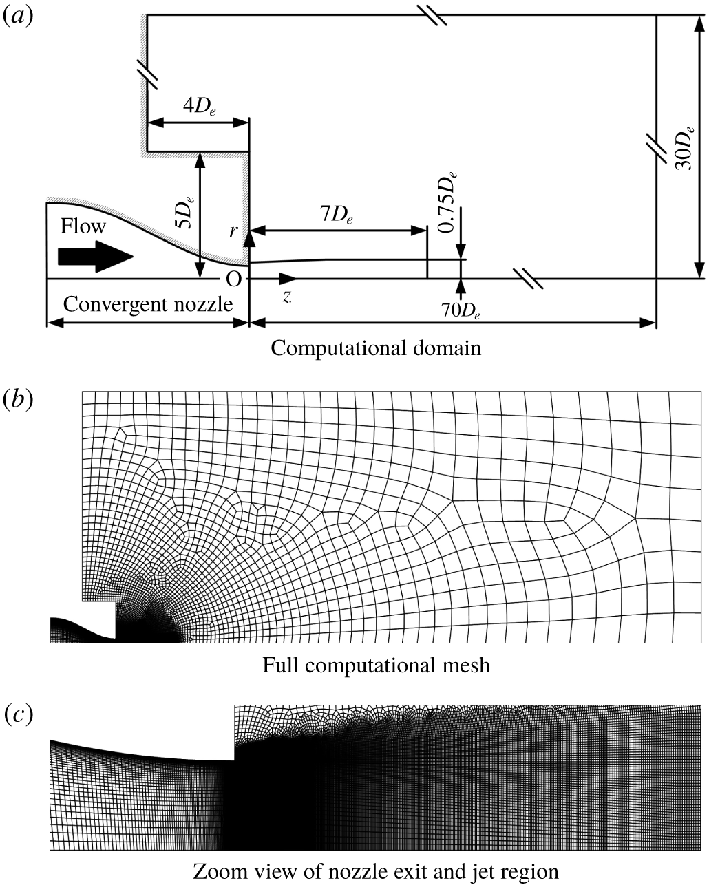
Figure 6. Computational domain and boundary conditions.
The numerical inlet and ambient conditions are identical to the experimental set-up in that the plenum pressure ( $p_{os}$) and temperature upstream of the nozzle are 405 kPa and 300 K, respectively, and the back pressure ( $p_{b}$) is set to atmospheric pressure, 101.3 kPa. The nozzle operating pressure ratio, $\text{NPR}=p_{os}/p_{b}$, is kept constant at 4.0. The dry air is assumed to be a perfect gas with a constant specific heat ratio of $\unicode[STIX]{x1D6FE}=1.4$, and the coefficient of viscosity is calculated by using Sutherland’s law. Figure 6(b) and 6(c) show the meshes of the entire computational domain and near the nozzle exit, respectively. The solid walls including the nozzle wall are treated as adiabatic and no-slip, and we use the pressure outlet condition (i.e. $p_{b}$ is specified) for the top and right boundaries. The structured mesh is generated by the mapped face meshing function equipped with ANSYS Fluent, and the total mesh count is approximately 50 000 elements. We generated relatively uniform and fine grids from $z=0$ to $7D_{e}$ in order to resolve the complex shock structures. Since our previous studies (Sugawara et al. Reference Sugawara, Nakao, Miyazato, Ishino and Rösgen2018) could not capture a Mach disk using the coarse mesh, we refined the mesh further, especially in the region where a Mach disk is supposed to be located. Inside the nozzle, the grid spacing smoothly reduces in the radial direction to capture the thin boundary layer. To capture the fine structures of the shock-containing microjets, we set a minimum mesh interval to ${\sim}2~\unicode[STIX]{x03BC}\text{m}$ in the vicinity of the nozzle exit. (Note that the spatial measurement resolution of the density is around $4~\unicode[STIX]{x03BC}\text{m}$.) The number of iterations is 10,000, at which the residuals of all equations (species, momentum, energy, turbulent kinetic energy $k$ and specific rate of dissipation $\unicode[STIX]{x1D714}$) reduce by three orders of magnitude, and the solutions seem to converge sufficiently. Here, the CFL (Courant–Friedrichs–Lewy) number is set to be small ( $=0.1$) due to the fact that a large CFL number results in undesired oscillations of the shock fronts, and thus the overall computational time increases.
We use the differentiable function as the limiter of the MUSCL scheme (monotonic upwind scheme for conservation laws) to achieve the third-order accuracy in space. Note that using the high-order scheme, which satisfies a total-variation-diminishing (TVD) condition, is particularly important for this type of application. The time integration is performed using the three-stage Runge–Kutta method. We performed a RANS grid dependence study (with the SST  $k$–
$k$– $\unicode[STIX]{x1D714}$ turbulence model) using different resolutions of the mesh (not shown here). We found that a refined mesh (the minimum mesh interval should be ${\sim}4~\unicode[STIX]{x03BC}\text{m}$) is required to accurately capture a Mach disk under the same flow conditions as in the present experiment. Considering that the results using minimum mesh intervals of $1~\unicode[STIX]{x03BC}\text{m}$ and $2~\unicode[STIX]{x03BC}\text{m}$ agree with each other satisfactorily, we decided to show the results with a minimum mesh interval of $2~\unicode[STIX]{x03BC}\text{m}$ for the rest of this study. Furthermore, not shown here, the flow field of a microjet was simulated by different models, inviscid (Euler), laminar and RANS with SST $k$–
$k$– $\unicode[STIX]{x1D714}$. We observed that the discrepancies between the experimental data and non-turbulence simulations (Euler and laminar) are relatively large and found a better agreement between the experimental data and RANS. For instance, the edge location of the shear layer by the laminar simulation remains almost constant in the downstream direction, while those of the present experiment and the RANS simulation decrease gradually towards downstream. The turbulence model seems to be capable of capturing the shear layer region in a more physically consistent manner for the present Reynolds number ( $Re_{d}=5.91\times 10^{4}$).
It should be noted that, as seen during the experiment, there are some unsteady motions that are overlooked in this steady calculation. Thus, a high-fidelity numerical simulation, such as large-eddy simulation, should be explored to capture unsteady features (Li et al. Reference Li, Zhou, Yao and Fan2017).
5 Results and discussion
5.1 Comparison of experimental results with simulations
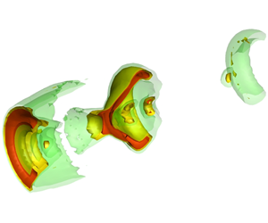
A comparison between the experimental measurement of the density contour plot at the cross-section including the jet centreline and the corresponding numerical result is depicted in figure 7. The contour levels with an interval of  $0.1~\text{kg}~\text{m}^{-3}$ are shown in the colour bar at the top, and the spatial resolution in the experimental density map is around $4~\unicode[STIX]{x03BC}\text{m}$. Figure 7 illustrates the various flow features of the shock-cell structures quantitatively, such as the shape and the size of the Mach disk in the first shock-cell as well as the expansion and compression regions, the shock-cell intervals, the jet boundaries, the slip streams produced from the triple points of a Mach disk and the shear layers outside of the jet boundaries. Although the unsteady features are ignored here and a relatively coarse mesh is used, there is very favourable overall agreement between the experiment and the simulation on the shock-cell structures. However, the simulation displays more distinct slip streams when compared with the experiment.
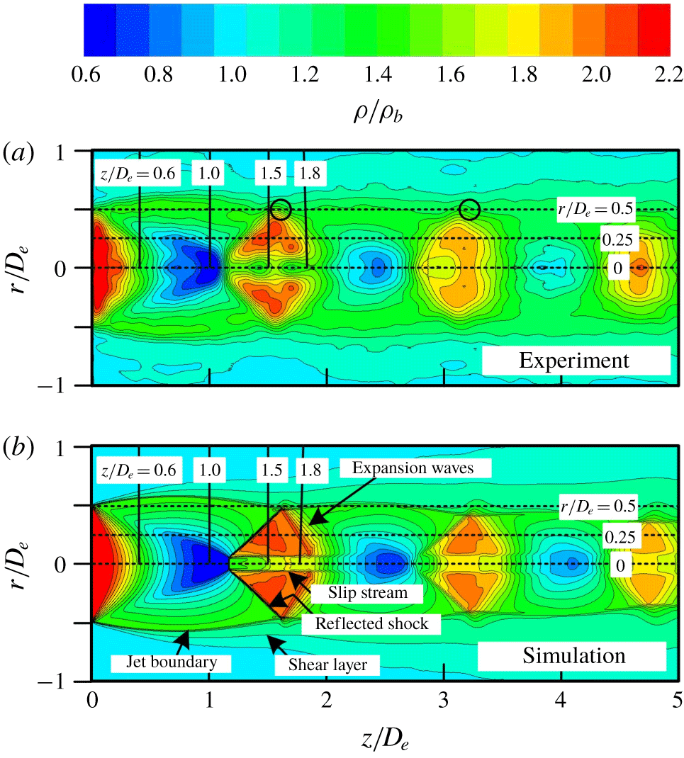
Figure 7. Density contours of underexpanded microjets.
The experimental data also show that the edge location of the shear layer remains almost the same ( $r=0.5~\text{mm}$) until the end of the domain, but the prediction does not. This discrepancy might be attributed to two issues: first, axial symmetry is assumed, and thus the nature of the fully three-dimensional effects could be overlooked; and second, the unsteady features are not captured by this RANS simulation. These issues should be investigated in the future. A Mach disk with a diameter of around $300~\unicode[STIX]{x03BC}\text{m}$ can be clearly recognized in the contour plots of the experiment and simulation of figure 7 in this study. This is consistent with the measurement done by André, Castelain & Bailly (Reference André, Castelain and Bailly2014), where the presence of a Mach disk with a small diameter in the first shock-cell is observed by the measurement using particle image velocimetry (PIV). The experiments by André et al. (Reference André, Castelain and Bailly2014) were performed under a nozzle pressure ratio of $\text{NPR}=3.67$ using an axisymmetric convergent nozzle with an inner diameter of 38.7 mm at the nozzle exit.
Figure 7(b) shows two distinct oblique shocks in the second shock-cell. Both of them originate from near the jet centreline and are towards the jet free boundaries. It is noteworthy that a second Mach disk can be observed indistinctly at the positions where the oblique shocks are produced. The slip streams produced from the intersections between the second Mach disk and the oblique shocks extend downstream keeping the shape almost parallel to the jet centreline. The existence of the third slip stream can be found in the third shock-cell. The presence of a second Mach disk was displayed in a velocity contour map obtained from PIV measurements by Edgington-Mitchell, Honnery & Soria (Reference Edgington-Mitchell, Honnery and Soria2014), who demonstrated that the shear layer originating from the triple point of the first Mach disk persists across multiple shock-cells downstream. Their experiment was performed at a nozzle pressure ratio of  $\text{NPR}=4.2$, which is slightly higher compared with our experimental condition ( $\text{NPR}=4.0$). However, the second Mach disk cannot be observed in figure 7(a). A more sophisticated instrumentation to investigate such a local phenomenon needs to be done.
It should be noted that the conventional schlieren and shadowgraph pictures sometimes show the incident shock or barrel shock just upstream of the Mach disk, but such a shock cannot be clearly seen in the contour plot representation at the jet cross-section for both the experiment and simulation in this study. Therefore, what was considered to be the incident shock wave or the barrel shock wave seen in the conventional pictures so far could be considered to be a compression wave, where there is a noticeable difference between density distributions integrated in the line-of-sight direction and those at the jet cross-section shown in figure 7. As described later, there is some evidence to support this conclusion.

Figure 8. Streamwise density profiles of underexpanded microjets.
A comparison between the experiment and the simulation of the streamwise density profiles at radial distances of  $r/D_{e}=0$, 0.25 and 0.5 is shown in figure 8(a–c), where the experimental results are represented with precision error bars. These radial locations are shown as the three horizontal dotted lines in the contour plots of figure 7. The density value at the nozzle exit plane, which is estimated based on the assumption of one-dimensional isentropic flow from the nozzle inlet to the exit, is shown as a leftward arrow on a vertical axis as a reference. The two-way vertical arrow indicates the ideal normal shock jump, which is estimated using the flow properties just upstream of a Mach disk with the assumption of an isentropic flow from the nozzle inlet to a Mach disk.
As a global feature, the experimental density profile in figure 8(a) exhibits a representative property appearing in an underexpanded free jet, i.e. the flow expansion and compression quasi-periodically repeated downstream are responsible for the shock-cell structures. In addition, the density rapidly decreases below the ambient level by expansion waves originating from the nozzle lip. The simulated density profile exhibits a similar trend as the experiment over the entire region except that the simulation shows a smoother density variation at the entire streamwise locations compared with the experiment.
Let us focus on the spatial variation of the centreline density profile behind a Mach disk. The experimental density profile in figure 8(a) shows two distinctive bumps (at  $z/D_{e}\simeq 1.2$ and 1.7) just downstream of a Mach disk, which are caused by the wavy behaviour with the divergence/convergence of the slip streams immediately after a Mach disk as clearly seen in figure 7(a). The first divergence of the slip streams leads to the rapid density rise after the density jump by a Mach disk because of the aerodynamic effect of the subsonic flow behind a Mach disk. The waveform with the two significant bumps behind a Mach disk also appears in the density profile obtained from the rainbow schlieren deflectometry by Takano et al. (Reference Takano, Kamikihara, Ono, Nakao, Yamamoto and Miyazato2016) as illustrated later in figure 12. Additionally, the similar waveform just downstream of a Mach disk can be observed in the velocity profile along the jet centreline obtained by PIV of André et al. (Reference André, Castelain and Bailly2014). However, such bumps cannot be seen in the simulated density profile. This may be due to the overlooked three-dimensional effects, unsteady flow features, and possible inadequacy of the current simulation model (e.g. coarse mesh). However, as can be seen in figure 8(a), the overall agreement between the measured and the simulated density profiles is favourable from the nozzle exit ( $z/D_{e}=0$) to the exit of the simulation domain ( $z/D_{e}=5$). Also, both the predicted shock-cell lengths and the density amplitudes agree well with the measurement quantitatively.
Figure 8(b) shows the measured and the simulated density profiles at the radial location of  $r/D_{e}=0.25$. Both of the density profiles capture the reflected shock wave, and the overall agreement between the experimental and the simulated results is satisfactory. Figure 8(c) shows the streamwise density profile along the jet lipline ( $r/D_{e}=0.5$). The experimental and the simulated density profiles show significant small bumps quasi-periodically appearing, which are marked as small black circles in the experimental density contour plot of figure 7(a). These bumps are responsible for the reflection as expansion waves of shock waves or compression waves at the jet boundaries. Again, good quantitative agreement for both of the density profiles is reached between experiment and simulation.
Comparisons between the experiment and the simulation for the radial density profiles along the four parallel vertical lines ( $z/D_{e}=0.6$, 1.0, 1.5 and 1.8) in the density contour plots in figure 7 are shown in figure 9(a–d). The dashed line parallel to the vertical axis indicates the density value estimated based on the assumption that the flow from the nozzle is isentropically expanded to the back pressure, which is referred to as the fully expanded jet density $\unicode[STIX]{x1D70C}_{j}$ and is estimated to be $1.75~\text{kg}~\text{m}^{-3}$ ( $\unicode[STIX]{x1D70C}_{j}/\unicode[STIX]{x1D70C}_{b}=1.48$) in this experiment. The solid and open circles shown on the experimental and the numerical density profiles in figures 9(a) and 9(b) are the radial positions of the local maximum and minimum values, respectively. The maximum density values in the simulated density profiles in both figures 9(a) and 9(b) are in quantitatively good agreement with the fully expanded jet density $\unicode[STIX]{x1D70C}_{j}$, and the corresponding radial positions nominally indicate the inviscid jet boundary (Panda & Seasholtz Reference Panda and Seasholtz1999). The density at the jet boundary approaches the ambient density $\unicode[STIX]{x1D70C}_{b}$ ( $=1.18~\text{kg}~\text{m}^{-3}$) through the shear layer radially outside of the boundary. It is noted that $\unicode[STIX]{x1D70C}_{j}$ is different from the ambient density $\unicode[STIX]{x1D70C}_{b}$ even though the fully expanded jet pressure $p_{j}$ has to coincide exactly with the back pressure $p_{b}$. Therefore, we conclude that the position of the local maximum in the density profile for the experiment seems to correspond to that of the inviscid jet boundary. As mentioned before, figure 9(b) demonstrates that the radial density profile just upstream of a Mach disk shows a smooth radial variation over from the local minimum value to the local maximum value. It means that no incident shock or barrel shock is present in front of a Mach disk, but instead compression waves appear. The experimental data of Panda & Seasholtz (Reference Panda and Seasholtz1999) also show the same trend.
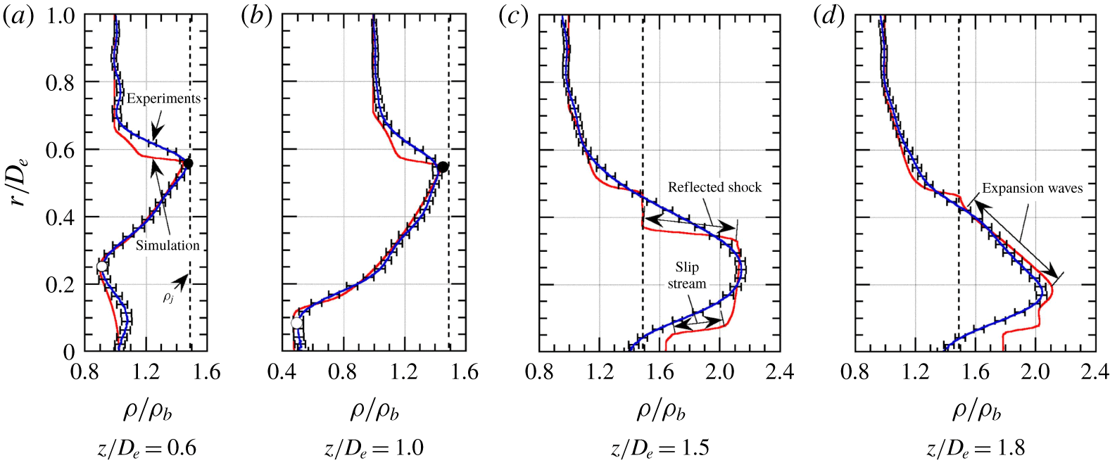
Figure 9. Radial density profiles of underexpanded microjets.
As shown in figure 9(c), the radial density profile passing through the middle of the reflected shock exhibits a noticeable discrepancy between the experimental and the simulated results. The experimental density profile is not capable of capturing a reflected shock wave, although the simulated density profile shows that the density remains uniform until it crosses the reflected shock and suddenly drops to the density at the inviscid jet boundary just downstream of the reflected shock. Such a gradual density variation across the reflected shock is also observed in the experimental density profile of Panda & Seasholtz (Reference Panda and Seasholtz1999), but the primary reason remains unclear at the present stage. The experimental density profile in figure 9(c) shows a smooth variation across the slip stream and it seems to be responsible for a mixing caused by a significant spreading of the slip stream opposed to a somewhat sharp variation of the simulated density profile. The simulated density sharply drops to the  $\unicode[STIX]{x1D70C}_{j}$ passing through the reflected shock and approaches the ambient condition via the shear layer after a region where the density remains constant at $\unicode[STIX]{x1D70C}_{j}$, while the experimental density profile shows a continuous variation between the reflected shock and the shear layer. In the radial density profiles downstream of the reflected shock shown in figure 9(d), relatively good agreement between the experimental and the simulated results is achieved, with the exception of the regions near the jet centreline.
Given the axisymmetric geometry, the density uncertainty may be affected by radial distance from the jet centreline. Behjat et al. (Reference Behjat, Tallents and Neely1997) demonstrated that the error in the densities deduced by the Abel inversion algorithm with the sixth-order polynomial fitting function for an axisymmetric jet increases towards the jet edges. Álvarez et al. (Reference Álvarez, Rodero and Quintero2002) also discussed the error introduced by the Abel inversion algorithm based on an exact solution including the ridge between the centre and outer edge, and further compared the exact solution with those analysed using different Abel inversion algorithms. It is shown that the Nestor–Olsen algorithm produces the highest error at the centre of the radial distribution and a few errors around the ridge, and that the discretization algorithm can reproduce the exact solution except for around the ridge. However, it should be noted that the studies of Behjat et al. (Reference Behjat, Tallents and Neely1997) and Álvarez et al. (Reference Álvarez, Rodero and Quintero2002) did not take into account a discontinuous variation caused by shocks in the distribution. Since it is not feasible to precisely estimate the density uncertainty attributed to only the Abel inversion algorithm for the case of the jets subject to unstable strong shocks, we have derived the precision errors based on the convolution back-projection (CBP) method (Decker Reference Decker, Lading, Wigley and Buchhave1994) and compared these errors with those from the Abel inversion method. Figure 10(a–d) shows the precision errors of jet radial densities at four different axial locations:  $z/D_{e}=0.6$, 1.0, 1.5 and 1.8. It is found that the errors are slightly larger for the Abel inversion method than for the CBP method. However, the errors from both methods remain almost constant inside the jet boundary and then gradually decrease in the radial direction. Note that these errors (or fluctuations) are caused by the coupling effects, such as: strong density fluctuations due to an oscillating Mach disk, associated oblique shocks and slip streams (Panda Reference Panda1998; Emami et al. Reference Emami, Bussmann and Tran2010; Edgington-Mitchell et al. Reference Edgington-Mitchell, Honnery and Soria2014; Li et al. Reference Li, Zhou, Chen, Fan and Xie2018). These effects could be more dominant than the measurement uncertainty. However, it is impossible to separate the uncertainty error from the effects causing the density fluctuations. Clarifying the unsteady behaviour of shock-containing jets would be one of the main objectives in our future works.

Figure 10. Comparison of precision errors for radial densities between Abel inversion method and CBP method.

Figure 11. Radial static pressure profiles obtained from RANS simulation for  $\text{NPR}=4.0$.

Figure 12. Comparison among centreline density profiles of underexpanded sonic jets obtained by various optical diagnostics for  $\text{NPR}=4.0$.
Figure 11 shows the radial static pressure profiles along four parallel vertical lines ( $z/D_{e}=0.6$, 1.0, 1.5 and 1.8) (see figure 7b). The horizontal axis is normalized by the back pressure $p_{b}$, which is the same as the fully expanded jet pressure $p_{j}$. As seen from a comparison between the simulated density and pressure profiles at the corresponding streamwise locations in figures 9 and 11, the static pressures coincide with the back pressure $p_{b}$ at the edge of the inviscid jet boundary indicated by the density profiles at $z/D_{e}=0.6$ and 1.0. For the simulated density profiles at $z/D_{e}=1.5$ (figure 9c) and 1.8 (figure 9d), for analogous reasons, the radial locations ( $r/D_{e}\simeq 0.4$ and 0.5, respectively), in which the static pressures and densities are equal to $p_{b}$ and $\unicode[STIX]{x1D70C}_{j}$, seem to be the inviscid jet boundaries. The static pressure in the jet shear layer is equal to the back pressure at all axial locations. This contrasts with the density at the inviscid jet boundary, which gradually decreases towards the ambient density.
5.2 Comparison of centreline density profiles obtained by various optical diagnostics
To obtain density data on shock-containing free jets, various non-intrusive experimental techniques have been presented in the past, including rainbow schlieren deflectometry (Satti et al. Reference Satti, Kolhe, Olcmen and Agrawal2007; Kolhe & Agrawal Reference Kolhe and Agrawal2009; Takano et al. Reference Takano, Kamikihara, Ono, Nakao, Yamamoto and Miyazato2016), background oriented schlieren (Venkatakrishnan Reference Venkatakrishnan2005; Van Hinsberg & Rösgen Reference Van Hinsberg and Rösgen2014; Nicolas et al. Reference Nicolas, Donjat, Léon, Le Besnerais, Champagnat and Micheli2017), moiré schlieren (Tabei, Shirai & Takakusagi Reference Tabei, Shirai and Takakusagi1992), Mach–Zehnder interferometer (Nakamura & Iwamoto Reference Nakamura and Iwamoto1996; Shimomiya et al. Reference Shimomiya, Ono and Miyazato2013), filtered Rayleigh scattering (Forkey et al. Reference Forkey, Lempert and Miles1998; Panda & Seasholtz Reference Panda and Seasholtz1999; Gustavsson & Segal Reference Gustavsson and Segal2005), coherent anti-Stokes Raman scattering (Woodmansee et al. Reference Woodmansee, Iyer, Dutton and Lucht2004) and dual-hologram interferometer (Velásquez-Aguilar et al. Reference Velásquez-Aguilar, Toker, Zamudio-Lara and Arias-Estrada2007). However, to the best of our knowledge, comparative studies between density data obtained with the same nozzle shape and under the same experimental conditions are virtually non-existent. Figure 12 shows a comparison between the density profiles along the jet centreline obtained using the various quantitative flow visualization methods for underexpanded sonic jets emitted from axisymmetric convergent nozzles under the same nozzle operating condition ( $\text{NPR}=4$) with different exit diameters. The density profiles normalized by the ambient density $\unicode[STIX]{x1D70C}_{b}$ from Tabei et al. (Reference Tabei, Shirai and Takakusagi1992), Nakamura & Iwamoto (Reference Nakamura and Iwamoto1996), Takano et al. (Reference Takano, Kamikihara, Ono, Nakao, Yamamoto and Miyazato2016) and Nicolas et al. (Reference Nicolas, Donjat, Léon, Le Besnerais, Champagnat and Micheli2017) are superimposed on our measurement (indicated by the blue line) using the Mach–Zehnder interferometer and the numerical result (indicated by the red line) from the RANS simulation with the SST $k$–
$k$– $\unicode[STIX]{x1D714}$ turbulence model. In order to make it easier to view, the precision error bars are removed from our experimental result and the theoretical density rise by a normal shock wave is also included as a reference.
Before comparing the present experimental and simulated results with previous experimental data, it is important to note that each methodology relies on certain assumptions and restrictions. The data acquired from the Abel inversion method are based on the assumption of an axisymmetric jet for the Mach–Zehnder interferometers and for the rainbow schlieren deflectometry. For the moiré schlieren method, the data measured by computed tomography with multi-viewing schlieren pictures are obtained by rotating a test nozzle around its longitudinal axis in equal intervals. Finally, the instantaneous density field reconstructed three-dimensionally with the simultaneous schlieren pictures is taken by mounting 12 synchronized cameras around a test nozzle for the background oriented schlieren.
What needs to be emphasized here is that, for the density profiles after the first and second shock-cells, the density value obtained from the Mach–Zehnder interferometer developed by Nakamura & Iwamoto (Reference Nakamura and Iwamoto1996) and that from the moiré schlieren developed by Tabei et al. (Reference Tabei, Shirai and Takakusagi1992) have an additional density increment compared to those from the other measuring techniques. The primary reason could be attributed to the oscillation of the shock position (Di Rosa, Chang & Hanson Reference Di Rosa, Chang and Hanson1993; Panda Reference Panda1998; Edgington-Mitchell et al. Reference Edgington-Mitchell, Honnery and Soria2014). When a shock wave oscillates across the time-mean position, the flow Mach number relative to the upstream-travelling shock is higher than that just ahead of the stationary shock. This results in an excessive density increment in addition to the density jump produced by the Rankine–Hugoniot relations. Other possible reasons could be the accuracy in the measuring techniques or the analytical method for reconstructing the density field.
As seen in figure 12, there is good quantitative agreement between the density profile obtained from the present Mach–Zehnder interferometer and those from both the rainbow schlieren deflectometry and the background oriented schlieren. The streamwise locations of the first and second local minima showing the ends of the expansion regions in the first and second shock-cells, respectively, and that of the second local maximum showing the end of the compression region in the second shock-cell, and the density values at their corresponding local minima and maximum, agree extremely well. In addition, the density behind a Mach disk in the first shock-cell for each density profile is almost the same peak value. The density profiles obtained from both the rainbow schlieren and the background schlieren show good quantitative agreement with the simulation over the entire region. It should be noted that the nozzle used by Takano et al. (Reference Takano, Kamikihara, Ono, Nakao, Yamamoto and Miyazato2016) is geometrically similar to that shown in figure 2, while the wall contour of the nozzle utilized by Nicolas et al. (Reference Nicolas, Donjat, Léon, Le Besnerais, Champagnat and Micheli2017) is converged in the downstream direction at a constant half-angle of  $30^{\circ }$ and followed by a short straight duct to provide a uniform sonic condition on the jet exit plane. From a comparison between the centreline density profile obtained by the present Mach–Zehnder interferometer and that by the rainbow schlieren deflectometry, it is important to note that there is almost no difference in effects of the nozzle size on the jet density field. Furthermore, the local minima in the density profiles for all of the experimental data as well as the simulation results gradually increase with increasing streamwise distance. This trend is also in good agreement with the results of Panda & Seasholtz (Reference Panda and Seasholtz1999) performed under almost the same experimental condition using filtered Rayleigh scattering.

Figure 13. Three-dimensional representation of shock surface of shock-containing microjet.
5.3 Flow topology of near-field shock systems
The shock dynamics of a shock-containing microjet can be quantitatively evaluated using the magnitude of the density gradient vector calculated by (Maeno et al. Reference Maeno, Kaneta, Morioka and Honma2005; Li et al. Reference Li, Zhou, Chen, Fan and Xie2018)
 $$\begin{eqnarray}|\unicode[STIX]{x1D735}\unicode[STIX]{x1D70C}|=\left[\left(\frac{\unicode[STIX]{x2202}\unicode[STIX]{x1D70C}}{\unicode[STIX]{x2202}x}\right)^{2}+\left(\frac{\unicode[STIX]{x2202}\unicode[STIX]{x1D70C}}{\unicode[STIX]{x2202}y}\right)^{2}+\left(\frac{\unicode[STIX]{x2202}\unicode[STIX]{x1D70C}}{\unicode[STIX]{x2202}z}\right)^{2}\right]^{1/2}.\end{eqnarray}$$
 This quantity seems to be capable of capturing inherent phenomena for a strongly underexpanded free jet including the interaction of shock waves with expansion waves. The density increases rapidly across a shock wave or the root of the Prandtl–Meyer expansion fan diverging from a sharp corner. Figure 13 shows a cutaway view of an isosurface of the three-dimensional density gradient field of the shock-containing microjet experimentally measured in this study. From figure 13, the spatial feature of the expansion fan emanating from the nozzle lip, the jet boundary, the short intercepting shock and the reflected shock can clearly be seen. Here, the Mach disk is around  $300~\unicode[STIX]{x03BC}\text{m}$ in diameter. It is found that the slip stream just behind the Mach disk is successfully captured in this three-dimensional view.
Figure 14 displays a bird’s-eye view of the magnitude of the density gradient vector on the cross-section including the centreline of the microjet. The flow topology as well as the shock strength are clearly shown. The Mach disk consists of shock systems where the shock strength reaches a maximum value at the centre and then decreases drastically towards the triple line (i.e. a triple point in a two-dimensional representation), while the reflected shock has some local maxima in the shock strength distribution, forming the wavy pattern. The slip stream expands initially just in the downstream region of the Mach disk followed by a rapid contraction. These results were also observed experimentally by Edgington-Mitchell et al. (Reference Edgington-Mitchell, Honnery and Soria2014) and numerically by Li et al. (Reference Li, Zhou, Chen, Fan and Xie2018). Since the flow is subsonic just behind the Mach disk, it decelerates initially and accelerates soon. This contributes to the behaviour of the divergence, and then it contracts in the streamwise direction of the area surrounded by the slip stream. We may conclude that our measurement technique with a high spatial resolution is capable of capturing the micrometre-scale shock dynamics in three-dimensional matter.

Figure 14. Density gradient field of shock-containing microjet.
6 Concluding remarks
The Mach–Zehnder interferometer system with the finite fringe method was applied for the first time to ‘quantitatively’ measure the density profiles over the whole density field of a shock-containing microjet. In this experiment, a nozzle pressure ratio defined as the ratio of the plenum to the ambient pressures was set to 4.0, which produces an underexpanded free jet with a Mach disk in the first shock-cell. The microjet structures were experimentally measured and demonstrated not only in the density contour plot at the cross-section including the jet centreline, but also in the streamwise and radial density profiles. In addition, the RANS simulation with the SST  $k$–
$k$– $\unicode[STIX]{x1D714}$ turbulence model was performed with the intent of a mutual comparison with the present experiment and to clarify the fine spatial features of the microjet structures.
It was shown that the experimental density contour plot illustrates the various flow features of the microjet, including the shape and size of the Mach disk as well as the expansion and compression regions, the shock-cell intervals, the jet boundaries, the slip streams produced from the triple points of the Mach disk and the outer shear layers near the jet boundaries. Very favourable overall agreement between the experiment and the simulation on the global shock-cell structures was found to be achieved.
More specifically, an excellent quantitative agreement is achieved between the experiment and the simulation for the streamwise density profiles at the jet centreline, the lipline and the intermediate line of them. Both of the simulated shock-cell lengths and density amplitudes are consistent with the measurement. From comparisons between the experiment and the simulation of the radial density profiles across the reflected shock wave in the first shock-cell, we can recognize the radial locations of the inviscid jet boundaries inside the shear layer. In the radial density profiles downstream of the reflected shock, the agreement between the experimental and the simulated results is not excellent, but is satisfactory. In the experimental density profile, the flow feature of the reflected shock wave shown in the simulation is missing.
The jet centreline density profile obtained from the present study was quantitatively compared with those from past studies such as the rainbow schlieren deflectometry, the background oriented schlieren, the moiré schlieren and Mach–Zehnder interferometer performed in the past. The centreline density profiles in underexpanded jets emitted from axisymmetric convergent nozzles for the same nozzle pressure ratio were demonstrated to investigate the effects of the nozzle exit diameters as well as how different measuring techniques work. It was found that the density profiles obtained from the present Mach–Zehnder interferometer, the rainbow schlieren deflectometry and the background oriented schlieren are in good quantitative agreement with each other except for some discrepancies just after a Mach disk. It is also shown that the simulated centreline density profile agrees well with those obtained from the present Mach–Zehnder interferometer, the rainbow schlieren and the background schlieren over the entire region from the first shock-cell to the third shock-cell. There is almost no difference in the effects of the nozzle size on the jet centreline density profile. However, at this stage, we cannot make firm conclusions about what causes the discrepancies seen in the density values just behind a Mach disk among the experiments, the simulations and normal shock theory. To elucidate the local phenomena at a higher level of complexity on shock dynamics, further experimental studies using more sophisticated instrumentation or high-fidelity numerical models (e.g. large-eddy simulation, direct numerical simulation, etc.) using a very fine mesh may be necessary.
The intricate patterns due to the interaction among shock waves, jet boundaries and expansion fans in the shock-containing microjet are quantitatively elucidated using the magnitude of the density-gradient vector within the microjet. The spatial feature of the complex shock structure can be clearly exhibited at a high spatial resolution of  $4~\unicode[STIX]{x03BC}\text{m}$ with the bird’s-eye view on shock strength. In addition, we observed that the microjet contains a Mach disk of around $300~\unicode[STIX]{x03BC}\text{m}$ diameter, a faintly visible intercepting shock surface and a well-defined reflected shock surface within the first shock-cell. The Mach disk consists of shock systems with the shock strength becoming a maximum value at the centre and then reducing drastically towards the triple line, while the reflected shock shows some local maxima on the shock strength distribution that forms the wavy pattern. Lastly, the unstable shear layer extending downstream from just behind the Mach disk oscillates and contributes to the formation of the wavy pattern of the density profile just behind the Mach disk.
The present study is the first trial of its kind among applications of Mach–Zehnder interferometers for micrometre-scale free jets including strong shocks, and it shows that the Mach–Zehnder interferometer with the finite fringe method proves to be a very efficient tool to investigate the fine structures of microjets with strong shock waves at a high spatial resolution. The present quantitative optical diagnostic can be applicable for time-dependent or asymmetric density fields too. The present experimental and numerical results could be useful for the validation of various numerical simulation codes for the case of shock-containing free jets under precisely identical operating conditions and nozzle configurations. The authors believe that the data presented here could be important for providing a database that can be used for further refinements of the computational efforts as well as for a mutual comparison among other non-intrusive techniques.
Acknowledgements
The authors are grateful to graduate student Taishi Takeshita of our laboratory for his assistance in the adjustment of the Mach–Zehnder interferometer. The authors also wish to express our deepest thanks to Dr Daisuke Ono for the development of the in-house software for reconstruction of the density fields from interference images. Without his persistent help, this research would not have been possible.
Declaration of interests
The authors report no conflict of interest.


 Open access