3.1. Method of optimal disturbances calculation

The idea of spatial optimal perturbations is to find such a perturbation that will lead to the greatest increase in the kinetic energy of a perturbation for a given axial coordinate $z$ and frequency. The study of the optimal perturbations begins with the search for eigenmodes of the jet velocity profile. The velocity components and pressure, with small perturbations, are substituted into the dimensionless equations of motion of a viscous, incompressible fluid:

(3.1)\begin{equation} \left.\begin{array}{c@{}} \boldsymbol{u}_t+(\boldsymbol{u}\boldsymbol{\cdot} \boldsymbol{\nabla})\boldsymbol{u}=-\boldsymbol{\nabla} p+\dfrac{1}{Re} \nabla^2\boldsymbol{u},\\ \boldsymbol{\nabla} \boldsymbol{\cdot} \boldsymbol{u} = 0, \end{array} \right\} \end{equation}

where $\boldsymbol {u}$ is the fluid velocity vector, $p$ is the pressure and $Re$ is the Reynolds number based on the maximum jet speed and the orifice radius. The subscript $t$ denotes the derivative with respect to the time $t$. After linearization with respect to perturbations, $\boldsymbol {u}=\boldsymbol {U}+\boldsymbol {u'}, p=P+p', \| \boldsymbol {u'} \|/\| \boldsymbol {U} \| \ll 1$, we get

(3.2)\begin{equation} \left.\begin{array}{c@{}} \boldsymbol{u'}_t+(\boldsymbol{U}\boldsymbol{\cdot} \boldsymbol{\nabla})\boldsymbol{u'}+(\boldsymbol{u'}\boldsymbol{\cdot} \boldsymbol{\nabla})\boldsymbol{U}=-\boldsymbol{\nabla} p'+\dfrac{1}{Re} \nabla^2\boldsymbol{u'},\\ \boldsymbol{\nabla} \boldsymbol{\cdot} \boldsymbol{u'} = 0, \end{array} \right\} \end{equation}

where $\boldsymbol {u'}$ is the fluid velocity perturbation, $p'$ is the pressure perturbation and $\boldsymbol {U} = U(r)\boldsymbol {e}_z$ is the base flow velocity field.

Following Khorrami, Malik & Ash (Reference Khorrami, Malik and Ash1989), perturbations are considered in the form of the eigenmodes in cylindrical coordinates $(r,\theta, z)$:

(3.3)\begin{equation} \left.\begin{array}{c@{}} \boldsymbol{u'}=\begin{bmatrix} u \\ v \\ w \end{bmatrix} (r, \theta, z, t) = {\rm e}^{{\rm i} (\alpha z + n \theta - \omega t)} \begin{bmatrix} iF \\ G \\ H \end{bmatrix} (r), \\ p'=p (r, \theta, z, t) = \, {\rm e}^{{\rm i} (\alpha z + n \theta - \omega t)} P (r), \end{array} \right\} \end{equation}

where $\alpha$ is the axial wavenumber, $n$ is the azimuthal wavenumber and $\omega$ is the frequency.

Given a real frequency $\omega$ and an integer azimuthal wavenumber $n$, the eigenvalue problem with respect to the axial wavenumber $\alpha$ is solved using the Chebyshev spectral collocation method. First, we substitute (3.3) into (3.2) to obtain the ordinary differential eigenvalue problem:

(3.4) \begin{align} &\begin{pmatrix} \dfrac{\partial}{\partial r} + \dfrac{1}{r} & \dfrac{n}{r} & 0 & 0 & 0 & 0 & 0\\ \varDelta & -\dfrac{2n}{r^2} & 0 & \mathrm{i}\,Re\dfrac{\partial}{\partial r} & 0 & 0 & 0\\ -\dfrac{2n}{r^2} & \varDelta & 0 & -\dfrac{\mathrm{i}\,Re\,n}{r} & 0 & 0 & 0\\ -\mathrm{i}\,Re\dfrac{\mathrm{d} U}{\mathrm{d} r} & 0 & \varDelta_z & 0 & 0 & 0 & 0 \\ 0 & 0 & 0 & 0 & 1 & 0 & 0 \\ 0 & 0 & 0 & 0 & 0 & 1 & 0\\ 0 & 0 & 0 & 0 & 0 & 0 & 1\\ \end{pmatrix} \begin{pmatrix} F \\ G \\ H \\ P \\ \alpha F \\ \alpha G \\ \alpha H \end{pmatrix} \nonumber\\ &\quad =\alpha \begin{pmatrix} 0 & 0 & -1 & 0 & 0 & 0 & 0\\ \mathrm{i}\,ReU & 0 & 0 & 0 & 1 & 0 & 0\\ 0 & \mathrm{i}\,ReU & 0 & 0 & 0 & 1 & 0\\ 0 & 0 & \mathrm{i}\,ReU & \mathrm{i}\,Re & 0 & 0 & 1\\ 1 & 0 & 0 & 0 & 0 & 0 & 0\\ 0 & 1 & 0 & 0 & 0 & 0 & 0\\ 0 & 0 & 1 & 0 & 0 & 0 & 0 \end{pmatrix} \begin{pmatrix} F \\ G \\ H \\ P \\ \alpha F \\ \alpha G \\ \alpha H \end{pmatrix}, \end{align}

where

(3.5a,b)\begin{equation} \varDelta = \dfrac{\partial^2}{\partial r^2} + \dfrac{1}{r}\dfrac{\partial}{\partial r} + \mathrm{i}\,Re\omega - \dfrac{n^2 + 1}{r^2}, \quad \varDelta_z = \dfrac{\partial^2}{\partial r^2} + \dfrac{1}{r}\dfrac{\partial}{\partial r} + \mathrm{i}Re\omega - \dfrac{n^2}{r^2}. \end{equation}

In (3.4), we increased the number of independent variables by adding $\alpha F, \alpha G, \alpha H$ in order to transform the system to a linear one in $\alpha$. The system (3.4) is supplied with the following boundary conditions. As $r\to +\infty$, we require the decay of perturbations:

(3.6)\begin{equation} F(+\infty) = G(+\infty) = H(+\infty) = P(+\infty) = \alpha F(+\infty) = \alpha G(+\infty) = \alpha H(+\infty) = 0. \end{equation}

At $r=0$, we require

(3.7)\begin{align} \left.\begin{array}{l} \text{if}\quad n = 0: \quad \begin{cases} F(0) = G(0) = \alpha F(0) = \alpha G(0) = 0,\\ \dfrac{\partial H}{\partial r}(0) = \dfrac{\partial \alpha H}{\partial r}(0) = 0,\quad \dfrac{\partial P}{\partial r} = 0; \end{cases}\\ \text{if}\quad|n| = 1: \quad \begin{cases} H(0) = P(0) = \alpha H(0) = 0,\\ F(0) + G(0) = 0,\quad \alpha F(0) + \alpha G(0) = 0,\\ 2\dfrac{\partial F}{\partial r}(0) + \dfrac{\partial G}{\partial r}(0) = 0, \quad 2\dfrac{\partial \alpha F}{\partial r}(0) + \dfrac{\partial \alpha G}{\partial r}(0) = 0; \end{cases}\\ \text{if}\quad |n| \geq 2: \quad F(0) = G(0) = H(0) = P(0) = \alpha F(0) = \alpha G(0) = \alpha H(0) = 0. \end{array}\right\} \end{align}

Second, we discretize the differential eigenvalue problem using the Chebyshev collocation method. The infinite domain is reduced to $0\le r \le R_{out}$, where $R_{out}$ is sufficiently large, and the boundary conditions (3.6) are set at $r=R_{out}$. After the Gauss–Lobatto grid is mapped upon the physical domain, we calculate the so-called Chebyshev differentiation matrix. For the computational domain $(-1, 1)$, the Chebyshev differentiation matrix of size $M$ has the following elements (Canuto et al. Reference Canuto, Hussaini, Quarteroni and Zang2007):

(3.8) \begin{equation} (D_M)_{j l}= \begin{cases} \dfrac{\bar{c}_j}{\bar{c}_l} \dfrac{(-1)^{\,j+l}}{x_j-x_l}, & j \neq l, \\ -\dfrac{x_l}{2(1-x_l^2)}, & 1 \leq j=l \leq M-2, \\ \dfrac{2 (M - 1)^2+1}{6}, & j=l=0, \\ -\dfrac{2 (M - 1)^2+1}{6}, & j=l=M - 1 ,\end{cases} \end{equation}

where $x_j=\cos ({{\rm \pi} j}/({M - 1}))$ for $j = 0,\ldots, M - 1$ and $\bar {c}_j = 2$ for $j = 0, M - 1$ and $\bar {c}_j = 1$ otherwise. For an arbitrary interval, the Chebyshev differentiation matrix can be calculated using the chain rule and (3.8). After that, we replace $\partial /\partial r$ with it in (3.4). Finally, we apply the boundary conditions (3.6), (3.7) and obtain the algebraic eigenvalue problem. More details of the Chebyshev collocation technique are presented in Trefethen (Reference Trefethen2000) and Canuto et al. (Reference Canuto, Hussaini, Quarteroni and Zang2007). The choice of $R_{out}$ and the grid size was based on a spectrum convergence study for each $n$ and $\omega$.

Thus, a set of eigenvalues and corresponding eigenvectors $\{\alpha _j, \boldsymbol {q}_j\}$ is found in the viscous linear formulation for the considered velocity profile. They include truly discrete eigenvalues, as well as a discretized continuous spectrum. An arbitrary perturbation can be represented as an expansion in eigenmodes:

(3.9)\begin{equation} \boldsymbol{q} (r, \theta, z, t) = \sum_{j = 1}^{N} \gamma_j \boldsymbol{q}_j (r) \,{\rm e}^{\mathrm{i} (\alpha_j z + n \theta - \omega t)}, \end{equation}

where $\boldsymbol {q} = (u, v, w, p)$ is the state vector of the system, $\alpha _j$ and $\boldsymbol {q}_j=(iF,G,H,P)$ are the $j$th eigenvalue and the corresponding eigenvector, respectively, and $N$ is the number of eigenmodes used in the calculations.

Disturbances with $\mathrm {Im}\, \alpha < 0$ are travelling upstream of the disturbance generator and are not included in this expansion, with the exception of discrete instability modes travelling downstream. There are zero, one or two instability modes for the considered velocity profile, depending on $\omega$ and $n$ (Gareev et al. Reference Gareev, Zayko, Chicherina, Trifonov, Reshmin and Vedeneev2022). To distinguish amplified downstream modes from decaying upstream modes (both have $\mathrm {Im}\, \alpha < 0$ for $\omega \in \mathbb {R}$), the following method was used. Due to the causality principle, as $\mathrm {Im}\, \omega \to +\infty$, all modes were unambiguously split into upstream ($\mathrm {Im}\,\alpha < 0$) and downstream ($\mathrm {Im}\,\alpha > 0$) travelling waves. For a fixed value of $\mathrm {Re}\, \omega$, we increased the value of $\mathrm {Im}\, \omega$ from zero to $\mathrm {Im}\, \omega >0$ and observed the motion of eigenvalues on the complex $\alpha$ plane, as shown in figure 3. While increasing $\mathrm {Im}\, \omega$, we selected eigenvalues $\alpha$ moving to the upper half-plane and consequently representing truly downstream-travelling waves. As intuitively expected, only instability modes associated with the inflection point of the velocity profile (Gareev et al. Reference Gareev, Zayko, Chicherina, Trifonov, Reshmin and Vedeneev2022), initially located at $\mathrm {Im}\,\alpha < 0$, moved to the upper half-plane and, hence, were included into the expansion (3.9). In calculations, we assume that the eigenmodes are sorted in ascending order of $\mathrm {Im}\,\alpha$ and choose the first $N$ modes for the expansion (3.9).

Figure 3. Loci of eigenvalues in the complex $\alpha$ plane with increase of $\mathrm {Im}\, \omega$ for $\mathrm {Re}\, \omega = 0.01, n = 1$. Dashed arrows show the motion of downstream-travelling damped modes, and the continuous arrow represents the downstream-travelling amplified mode. Red curve separates downstream- and upstream-travelling modes.

As a functional norm for which the optimization problem is solved, we consider the kinetic energy of perturbation:

(3.10)\begin{equation} E(z)=\frac{1}{4{\rm \pi} T}\int_0^\infty \int_0^T \int_0^{2{\rm \pi}} ((\mathrm{Re}\,u)^2+(\mathrm{Re}\,v)^2 +(\mathrm{Re}\,w)^2) r\, {\rm d} \theta\, {\rm d} t\, {\rm d} r, \quad T = \frac{2{\rm \pi}}{\omega}. \end{equation}

For stationary perturbations, we analyse the limit of $\omega \to 0$. To normalize initial kinetic energy of perturbations, we assume that $E(0)=1$.

After substituting (3.9) into (3.10), the kinetic energy of the perturbation (3.9) is expressed as a quadratic function of the expansion coefficients:

(3.11)\begin{equation} E(z; \boldsymbol \gamma) = \sum_{j, k = 1}^{N} \gamma_j^* E_{jk} \gamma_k = \boldsymbol{\gamma}^{{{\dagger}}} \boldsymbol{E}(z) \boldsymbol{\gamma}, \end{equation}

where $*$ represents complex conjugation, ${\dagger}$ is the Hermitian conjugation operator, $\boldsymbol {\gamma }$ is the column vector of coefficients of the expansion (3.9) and the components of the matrix $\boldsymbol {E}(z)$ are as follows:

(3.12)\begin{equation} E_{i j}=\tfrac{1}{4} \exp((-\mathrm{i} \alpha_i^{*} + \mathrm{i} \alpha_j)z ) \int_{0}^{\infty}(F_{i}^{*} F_{j}+G_{i}^{*} G_{j}+H_{i}^{*} H_{j}) r \,\mathrm{d} r. \end{equation}

Thus, the problem of optimal perturbations is reduced to the problem of constrained optimization (Boronin et al. Reference Boronin, Healey and Sazhin2013):

(3.13)\begin{equation} \boldsymbol{\gamma}^{{{\dagger}}} \boldsymbol{E}(z) \boldsymbol{\gamma}\boldsymbol \to \max, \quad \text{subject to}\ \boldsymbol{\gamma}^{{{\dagger}}} \boldsymbol{E}(0) \boldsymbol{\gamma} = 1. \end{equation}

The problem (3.13), in its turn, is reduced to the generalized Hermitian eigenvalue problem

(3.14)\begin{equation} \boldsymbol{E}(z) \boldsymbol{\gamma} = \sigma \boldsymbol{E}(0)\boldsymbol{\gamma}, \end{equation}

with its largest eigenvalue $\sigma _{max}$ being exactly the optimal energy value $E(z)$ for a given $z$. The value of $\sigma _{max}$ is found by the power iteration algorithm.

Summarizing, the algorithm for the calculation of the optimal perturbation for a given $z$ is as follows. After the calculation of the eigenvalues $\alpha _j$ and corresponding eigenvectors, we select those corresponding to downstream-travelling modes. Next, we calculate the matrices $\boldsymbol {E}(z)$ and $\boldsymbol {E}(0)$ and find the largest eigenvalue of the problem (3.14), which is the optimal perturbation energy. The corresponding eigenvector $\boldsymbol {\gamma }$ is used to calculate the initial and final spatial distributions (3.9) of the optimal perturbation. For every $n$ and $\omega$, we performed the convergence study in the number of downstream-travelling eigenmodes $N$ used in the expansion (3.9). Here $N$ was changed from 200 to 1500 to check the convergence.

3.2. Calculation results

Boronin et al. (Reference Boronin, Healey and Sazhin2013) showed that for several types of jet velocity profiles, stationary perturbations (that is, perturbations with $\omega \to 0$) demonstrate the largest non-modal growth. The same effect was obtained for the profile under consideration. Examples are shown in figures 4 and 5, where the ratio of the maximum relative kinetic energy $G$ of all perturbations,

(3.15)\begin{equation} G(z)=\max \frac{E(z)}{E(0)}, \end{equation}

to the energy of the fastest-growing eigenmode (denoted as $E_m$ in figures 4 and 5) reaches its maximum as $\omega \to 0$. Therefore, in what follows, we restrict ourselves to the stationary optimal perturbations.

Figure 4. The ratio of the optimal perturbation energy to the energy of the fastest-growing eigenmode for various frequencies for $n = 1$: (a) $z/D \le 5$; (b) $z/D \gg 1$.

Figure 5. The ratio of the optimal perturbation energy to the energy of the fastest-growing eigenmode for various frequencies for $n = 5$: (a) $z/D \le 5$; (b) $z/D \gg 1.$

Note that in our study we consider steady perturbations, i.e. $\omega \rightarrow 0$. It is known that for $\omega =0$, all eigenmodes of the linearized Navier–Stokes equations are either damped or neutral (it was also checked for our jet velocity profile). Consequently, the perturbation growth a priori cannot be generated by a single mode, and in this sense it is ‘non-modal’ by definition. Hence, the growth of a steady perturbation downstream can only be explained by a limited growth of a combination of damped modes. Such a combination can indeed grow due to non-self-adjointness of the linearized Navier–Stokes operator, and non-orthogonality of its eigenvectors (see Schmid & Henningson (Reference Schmid and Henningson2001) for details).

Figure 6 shows $G(z)$ for various azimuthal wavenumbers. Each curve in figure 6 depicts the envelope of the family of curves for the relative kinetic energy of all possible stationary perturbations for a given $n$. It can be seen that, for small values of $z$, perturbations with different $n$ grow at similar rates, but as $z$ increases, smaller $n$ corresponds to larger perturbation growth. For classical velocity profiles, non-modal growth of axisymmetric perturbations, $n=0$, due to the Orr mechanism, is significantly weaker than for $n\not =0$, where the ‘lift-up’ mechanism is active (Jiménez-González et al. Reference Jiménez-González, Brancher and Martínez-Bazán2015). The same result is obtained for our velocity profile: for axisymmetric perturbations $n = 0$, the optimal energy gain $G$ is less than $81$ for all $z$.

Figure 6. Energy growth of stationary optimal perturbations for various azimuthal numbers $n$: (a) $z/D \le 5$; (b) $z/D \gg 1.$

Since the unperturbed profile is axisymmetric, for each $n \neq 0$ there is a helical solution twisted counterclockwise, and a similar solution twisted in the opposite direction for $-n$. To get the optimal solution without twist, we average two helical perturbations:

(3.16)\begin{equation} \tilde{\boldsymbol{q}}^{n}(r, \theta, z) = \frac{\boldsymbol{q}^{n} (r, \theta, z) + \boldsymbol{q}^{-n} (r, \theta, z)}{2}, \end{equation}

where $\boldsymbol {q}^{n}$ is the optimal perturbation for a given $n$ and $\omega \to 0$. Three optimal perturbations, two with twist in opposite directions and one without twist, have the same optimal energy gains $G(z)$.

Visualizations of the untwisted optimal perturbations for $z$, where $G(z)$ reaches its maximum, are shown in figure 7, where the axial velocity perturbation is shown in colour, the streamlines are drawn for transverse velocities and the white circle is the unperturbed jet boundary.

Figure 7. Distribution of the axial component of the optimal perturbation velocity and streamlines in the jet cross-section for (a) $n=1$, (b) $n=2$, (c) $n=3$ and (d) $n=5$. The coordinate $z$ corresponds to the cross-section, in which the global energy maximum is reached: $z/D=1015$ for $n = 1, z/D=81$ for $n = 2, z/D=35$ for $n = 3$ and $z/D=12$ for $n = 5$.

As can be seen, the cases $n = 1$ and $n > 1$ differ in their spatial structure. In the case of $n = 1$, the optimal perturbation takes the form of a displacement mode whose effect is to shift the jet. This is called the ‘shift-up’ effect by Jiménez-González et al. (Reference Jiménez-González, Brancher and Martínez-Bazán2015). Due to the transfer of faster zone from the jet core to the shear layer, this shift leads to an increase and decrease in the axial velocity in two opposite shear regions. In the case of $n > 1$, the optimal perturbation consists of several vortex structures (the number of which is $2n$) that form ‘petals’ of jet acceleration and deceleration due to the replacement of fast zones by slow ones and vice versa. This structure resembles the ‘lift-up’ effect in the boundary layer.

An example of axial and transverse perturbation velocities for $n = 2$, which are optimal in some section, is shown in figure 8 as a function of the axial coordinate $z/D$ at $2r/D = 0.75$ (qualitatively similar distributions are observed in other points for all $n>0$). It can be seen that the axial velocity perturbation increases almost linearly up to $z/D \approx 4$ and just slightly deviates from the linear trend for $z/D>4$, while the two other velocity components almost do not change. These properties, the linear growth of the axial velocity perturbations with the preservation of longitudinal vortices, are characteristic of the non-modal ‘lift-up’ mechanism of the perturbation growth. As the axial velocity initially evolves almost linearly, and it is the dominant component of the kinetic energy of optimal perturbations, $E(z)$ grows almost quadratically with the increase of $z$.

Figure 8. Root mean square of the velocity component fluctuations of the optimal perturbation as $\omega \to 0$ for $n = 2$ at $2r/D = 0.75$.

Like the jet flows considered by Boronin et al. (Reference Boronin, Healey and Sazhin2013) and Jiménez-González & Brancher (Reference Jiménez-González and Brancher2017), the optimal perturbations for the considered profile have a complex three-dimensional structure and, accordingly, are difficult to implement in experiments. Nevertheless, in this experimental work, by using special deflectors, we create perturbations that are qualitatively close to the theoretical optimal ones.

4.1. Creation of disturbances

As described above, stationary perturbations have larger non-modal growth than non-stationary ones. That is why disturbances were introduced into the jet using motionless thin wave-like structures, which we call deflectors (figure 9).

Figure 9. Three-dimensional model (left) and printed deflector (right) with azimuthal wavenumbers $n = 3$ (a) and $n = 5$ (b), with parameters $\varepsilon = 0.1, d_0 = 60$ mm.

The upper edge of the deflectors was a circle of radius $r_0=d_0/2$ (${=}30$ mm in most of the experiments), and the lower edge is a perturbed circle with a given azimuthal wavenumber $n$ and radius $r=r_0(1 + \varepsilon \sin (n\theta ))$, where $\varepsilon$ defined the dimensionless amplitude of deviation from the circle and $\theta$ was a polar angle. The height of the deflector between the upper and lower edges is $h=10$ mm while the wall thickness was 0.6 mm. A smooth transition was made between the edges (points of the upper and lower edges with the same azimuthal coordinate $\theta$ were connected by straight-line segments). The models were designed in a computer-aided design program and then three-dimensionally printed from polylactic acid plastic.

A special holder was designed for the deflector installation inside the jet. This holder was attached to the diffuser like a crimp ring and allowed us to vary the distance between the orifice of the diffuser and the plane where the deflector was located, as well as the rotation angle of the deflector around the jet axis. The lower edge of the deflectors lay on strained fishing lines of 0.05 mm in diameter. The deflectors were installed inside the jet coaxially, with the inlet edge at a distance of $z=20$ mm, i.e. at $z/D=1/6$ (hereinafter, $z$ denotes the distance from the diffuser orifice), and the undisturbed inlet circle edge upwards. A photograph of the holder with the deflector installed is shown in figure 10.

Figure 10. Picture of the deflector holder.

4.2. Flow visualization method

Flow visualization (figure 11) was performed using the laser sheet method. Fine glycerol particles (of diameter 1–3 $\mathrm {\mu }$m) were introduced to the pipeline before the jet-forming device. A continuous green laser with a wavelength of 532 nm, equipped with a cylindrical lens to create a plane, illuminated the cross or longitudinal sections of the jet. Due to eventual settling of glycerol particles on the bushing with grids (of a cell size of 30–50 $\mathrm {\mu }$m), the bushing was regularly washed with water to maintain the characteristics of the jet. The video camera was located outside the flow and was mounted on a vertical traverse system together with the laser. Accordingly, it moved synchronously with the illuminated cross-section of the jet to ensure the same frame scale for each shooting distance. All frames of the cross-section at distances $z/D = 0.5\unicode{x2013} 3.5$ were obtained at an angle to the jet axis, so that a linear transformation of the frame plane was subsequently performed to eliminate its distortion.

Figure 11. Flow visualization scheme in longitudinal (a) and transverse (b) planes. Diffuser (1), glycerin aerosol generator (2), laser sheet (3), laser (4), video camera (5), holder with deflector (6).

4.3. Hot-wire anemometer measurements

Measurement of the instantaneous and averaged flow velocity was conducted using a hot-wire anemometer (DISA CTA BRIDGE 56C17). The hot-wire anemometer probe with 5 $\mathrm {\mu }$m tungsten wire was located at the end of the L-shaped holder (figure 12), whose movement in the transverse and axial directions of the jet flow was controlled from a PC. The signal was digitized by an analogue-to-digital converter at a frequency of 7500 Hz, which provided a fairly wide spectrum of velocity disturbances and negligible random measurement errors. A systematic absolute error of velocity measurements due to the calibration procedure was nearly 0.015 m s$^{-1}$, which corresponded to ${\sim }1\,\%$ relative error with respect to the maximum velocity of the base flow. Another source of errors was the five-second averaging time period, which was sufficient to show a trend in the evolution of disturbance, but could possibly have been sensitive to large-scale air motion in the test room.

Figure 12. Scheme for measuring the flow velocity with a hot-wire anemometer.

4.4. Particle image velocimetry measurements

The flow seeding method for particle image velocimetry (PIV) measurements was the same as for the flow visualization. The flow was illuminated with a Beamtech Vlite-Hi-100 high-frequency pulsed Nd:YAG laser mounted on a traverse system. A rod with an Allied Vision Bonito CL-400B high-speed PIV camera was also attached to the traverse system. When the cross-section was measured, the camera was placed directly into the jet at a distance of 720 mm (${\rm \Delta} z/D=6$) below the measured cross-section (figure 13). The camera installation scheme for measuring the longitudinal section is similar to that used for visualization (figure 11a). As the flow velocity in the regime under study did not exceed 1.5 m s$^{-1}$, and the delay between two flashes of the pulsed laser did not exceed 750 $\mathrm {\mu }$s, it was possible to detect the motion of particles in the transverse plane of the laser sheet (thickness not less than $0.001$ m). This design allowed shooting at distances $z/D=1\unicode{x2013} 2$. Shooting double frames was performed mainly at a frequency of 20 Hz.

Figure 13. Scheme of PIV experiments (cross-section of the jet). Diffuser (1), glycerine aerosol generator (2), laser sheet (3), high-frequency pulsed laser (4), high-speed camera (5), holder with deflector (6), traverse system (7).

Photo processing was performed using ActualFlow software and consisted of applying an iterative cross-correlation algorithm to find velocities in the $64\times 64$ pixel areas with 50 % overlap and subsequent filtering of the vectors by the signal-to-noise ratio, as well as by the magnitude of the components of the instantaneous velocity vectors. We did not seed the air surrounding the jet. Because of this, in the right-hand part of the velocity field patterns outside the jet, we could detect a parasitic high-velocity flow region remaining after filtration, which was explained by the camera noise (see figure 14a).

Figure 14. Velocity fields of the undisturbed flow obtained using PIV: (a) flow in the cross-section of the jet; (b) flow in a longitudinal section.

The average velocity field was found by averaging 3000 instantaneous velocity fields, so the random error was negligible. The systematic error came from the error of the cross-correlation algorithm, which could be estimated as ${\sim }1\,\%$. An example of the obtained transverse velocity modulus field in a jet is given for an undisturbed flow in figure 14(a) and for the axial velocity field in figure 14(b).

Each experiment consisted of putting a deflector into the flow and measuring the average axial velocity in the central plane of the jet, or the average transverse velocity at distances from the forming device orifice $z/D = 1, 1.25, 1.5, 1.75, 2$. These fields can be used to estimate the evolution of the flow disturbance downstream. In what follows, for brevity, flow patterns for $z/D = 1, 1.5, 2$ are given.

5.1. Visualization of the cross-section of the jet

To study the development of perturbations introduced by deflectors with $\varepsilon = 0.1$, experiments were conducted with the visualization of the cross-sections of the jet by a laser sheet.

Disturbances introduced by deflectors with initial diameter $d_0=60$ mm ($d_0=D/2$) developed faster and turbulized the flow earlier upstream compared with disturbances introduced by deflectors with $d_0=30, 90, 120$ mm. This can possibly be explained by a rather large unperturbed velocity at $r=30$ mm ($2r/D= 1/2$) and its large gradient (figure 2). Deflector configurations with larger or smaller $d_0$ introduce disturbances either where the velocity gradients are smaller or where the flow velocity is significantly less than the velocity at the jet centre.

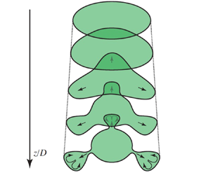
Disturbances caused by deflectors at small distances almost do not deform the cross-section, but the cross-section changes with the development of the stationary disturbance downstream, acquiring the shape of the outlet edge of the deflectors (figure 15). ‘Petals’ increase, stretch in the radial direction from the jet axis and form a ‘neck’ – a narrow region of the jet section connecting the petal with the jet core. Shortly after the formation of necks, a rapid growth of unsteady fluctuations and transition to turbulence at distances $z/D$ ${\sim }3$ are observed. A qualitative scheme for the development of such perturbations is shown in figure 15.

Figure 15. Three-dimensional models of deflectors with azimuthal numbers $n=3, 4, 5$ (a) and the evolution of stationary perturbations introduced by them as cross-section photographs (b) and the qualitative scheme (c).

Petal lengths versus the distance $z$ were obtained from the cross-section pictures of the jet for deflectors with $n=3$, 4, 5, and the resulting plots are shown in figure 16. Since one photograph of the instantaneous jet cross-section is analysed for each streamwise position, we estimate the uncertainty of this method (due to random fluctuations of the jet and air motion in the test room) as $<5$ %, which is acceptable to characterize the evolution of the perturbed jet. The lengthening of the petals occurs linearly; therefore, the radial velocity perturbation is approximately constant, which is consistent with the theoretical calculations of stationary optimal perturbations of the jet (§ 3.2).

Figure 16. (a) Measurement of the petal length in the jet cross-section perturbed by deflector with $n=5, \varepsilon =0.1$ at $z=1.5D$. (b) The petal length as a function of $z/D$. Perturbations with $n=3$ (grey squares), $n=4$ (green circles), $n=5$ (black diamonds).

5.2. Development of the axial velocity component

To make sure that the development of perturbations introduced by the deflectors qualitatively corresponds to the development of optimal perturbations, we considered the change in the axial flow velocity downstream. A series of experiments was performed to determine the average velocity with a hot-wire probe outside the flow core with deflectors for $n=3$, 4, 5 and $\varepsilon =0.05$ (figure 17) and $\varepsilon =0.1$ (figure 18). Points with constant radial and azimuthal coordinates were selected outside of the deflector wake.

Figure 17. Normalized axial velocity perturbation versus the distance $z$ downstream. Perturbations are introduced by a deflector with $\varepsilon =0.05$. Measurements in petals at $2r/D=0.8$ (a) and troughs at $2r/D=0.55$ (b). Perturbations with $n=3$ (grey squares), $n=4$ (green circles), $n=5$ (black diamonds).

Figure 18. Normalized axial velocity perturbation versus the distance $z$ downstream. Perturbations are introduced by a deflector with $\varepsilon =0.1$. Measurements in petals at $2r/D=0.8$ (a) and troughs at $2r/D=0.55$ (b). Perturbations with $n=3$ (grey squares), $n=4$ (green circles), $n=5$ (black diamonds).

In figures 17 and 18, the relative amplitudes of stationary disturbances versus $z/D$ are given at the points corresponding to petals of the jet section (left-hand panels) and corresponding to ‘troughs’ (right-hand panels). It is seen that in regions of contraction and expansion of the cross-section, the axial velocity evolves algebraically and close-to-linearly with streamwise distance. The significant deviation from the linear growth appears only for deflectors with $\varepsilon =0.1$ in petals of the jet at $z/D > 2.0$. The velocity, reaching its peak at $z/D \approx 2.0$, decreases, which is explained by the growth of nonlinear effects that arise when a sufficiently large perturbation amplitude is reached; namely, by the formation of necks. Close-to-linear growth of the axial velocity is in accordance with the development of theoretical optimal perturbations (§ 3.2).

5.3. Particle image velocimetry experiments

This section presents the results of PIV measurements in the transverse and longitudinal cut planes of the jet. Below, we show averaged perturbation fields, i.e. the disturbed flow minus the base flow. The streamlines of the transverse disturbance velocity are superimposed on the colour fields of the transverse disturbance velocity or vorticity magnitude. Flow patterns in transverse sections demonstrate the qualitative nature of the disturbance, and are given in dimensional quantities: m s$^{-1}$ and s$^{-1}$ for velocity and vorticity, respectively.

5.3.1. Flow in the transverse jet plane at $n=1\ldots 5$

Case of $\boldsymbol {n=1}.$ Figure 19 shows flow patterns with plotted streamlines for perturbation with $n=1$, taken at $z/D = 1$. Figure 19(a,b) shows the transverse velocity (colour denotes the velocity modulus) and figure 19(c,d) the values of the longitudinal vorticity component $\omega _z$. The thicker parts of the streamlines correspond to a larger modulus of transverse velocity. The large grey dashed ring has a diameter of 120 mm and corresponds to the boundary of the undisturbed jet and the small white curve corresponds to the location of the deflector outlet with real magnitude of $\varepsilon$. Figure 19(a,c) corresponds to a smaller flow disturbance caused by a deflector with $\varepsilon =0.05$ and figure 19(b,d) corresponds to the case $\varepsilon =0.1$. These deflectors shift the flow apart from the jet axis (for $n=1$, the deflector inlet as a dash-dotted circle is shown too), but the appearance of several regions with high vorticity should also be noted. At $\varepsilon = 0.05$, two symmetrically located and clearly distinguishable regions with opposite vorticities are observed; at $\varepsilon = 0.1$, the number of vorticity zones increases, they become larger and the maximum values of vorticity increase.

Figure 19. Transverse velocity (a,b) and vorticity (c,d) with plotted streamlines for perturbation with $n=1, z/D=1$ and $\varepsilon =0.05$ (a,c) or $0.1$ (b,d). The grey dashed circle is the unperturbed jet boundary, orange dash-dotted circle is the deflector inlet, white solid circle is its outlet.

Case of $\boldsymbol {n=2}.$ The outlet cross-section for the deflector with $n=2$ is characterized by two minima and two maxima, which are also reflected in the disturbance patterns (figure 20). In the directions of the maximum radii of the deflector, there is a flow from the axis to the periphery. For the radius minima, the opposite flow towards the axis is seen. Vortices are observed between these regions, which can be easily detected by the vorticity maxima in figure 20(c,d). For $\varepsilon =0.1$, the distribution of the modulus of velocity and vorticity is more complicated than for $\varepsilon =0.05$, which is probably explained by the appearance of nonlinear effects in the flow. That is, between the main zones of vorticity, additional vortex pairs arise in the directions of both deflector ‘maximum’ and ‘minimum’. As $\varepsilon$ increases from 0.05 to 0.1, the perturbation shrinks in the ‘minima’ direction, where the air flows towards the axis, and expands in the direction of the ‘maxima’, where the fluid is ejected to the periphery.

Figure 20. Transverse velocity (a,b) and vorticity (c,d) with plotted streamlines for perturbation with $n=2, z/D=1$ and $\varepsilon =0.05$ (a,c) or $0.1$ (b,d). The legend is the same as in figure 19. White solid curve is a perturbed circle (deflector outlet).

Case of $\boldsymbol {n=3}.$ For $n=3$, the flow pattern (figure 21) is essentially similar to the previous cases: each of the three perturbation petals produces two surrounding vortices, which capture fluid in the region of the small axial velocity located on the periphery, and transfer it towards the jet axis. They also transfer fluid from the region of high axial velocity near the axis to the periphery. Passing from $\varepsilon =0.05$ to $\varepsilon =0.1$, the maximum velocity and vorticity moduli increase, the flow in the petals becomes more complicated and significantly inhomogeneous and additional vorticity zones appear.

Figure 21. Transverse velocity (a,b) and vorticity (c,d) with plotted streamlines for perturbation with $n=3, z/D=1$ and $\varepsilon =0.05$ (a,c) or $0.1$ (b,d). The legend is the same as in figure 19.

Case of $\boldsymbol {n \ge 4}.$ Further increasing of $n$ gives the same flow patterns (figures 22 and 23 show an example of $n=5$). There is a general tendency to change the angle of inclination of the elongated vortex regions with an increase of $\varepsilon$: the vortex zones become more intensive and more aligned to the radial direction. For $\varepsilon =0.1$, the internal vortices observed for $n \le 3$ disappear, and only one pair of counter-rotating vortices is noticeable in each petal.

Figure 22. Perturbation evolution downstream for $n=5, \varepsilon =0.05$. The transverse velocity modulus (a–c) and vorticity (d–f) for (a,d) $z/D=1$; (b,e) $z/D=1.5$; (c,f) $z/D=2$.

Figure 23. Perturbation evolution downstream for $n=5, \varepsilon =0.1$. The transverse velocity modulus (a–c) and vorticity (d–f) for (a,d) $z/D=1$; (b,e) $z/D=1.5$; (c,f) $z/D=2$.

5.3.3. Measurements in the longitudinal plane

The measurements described in the previous section show how the transverse velocity and vorticity evolve, but do not provide information about the axial component of the disturbance. To obtain the corresponding velocity fields, a series of experiments was performed, in which the laser sheet passed through the jet axis and the camera obtained flow patterns in the meridional plane.

Due to their symmetries, deflectors give a different number of characteristic planes in which measurements should be made to study the flow patterns. For odd $n=1, 3, 5,\ldots,$ when a plane passes through an antinode, there will also be an antinode of the opposite kind (maximum–minimum and vice versa), and it is enough to make one measurement in order to investigate the development of a petal of the disturbance. For even $n=2, 4,\ldots$, there are planes of symmetry passing through antinodes of the same type (maximum–maximum, minimum–minimum), so that in this case, measurements in two planes are made.

Below, as an example, longitudinal perturbation patterns with $n=2$ and 3 for $\varepsilon =0.1$ are given. For convenience, the axis perpendicular to the $z$ axis in the cut plane is denoted by $x$.

Figure 24 shows two perturbation velocity fields obtained in the maximum–maximum (figure 24a) and minimum–minimum (figure 24b) planes for $n=2$. The arrows show the perturbation velocity vectors, and the colour fill corresponds to its axial component $u_z$ normalized by the maximum value of the base flow axial velocity $U_c$. In figure 24(a), the jet expands, and the axial component of the velocity increases downstream. A small reverse perturbation velocity arises in the flow core. In the minimum–minimum plane (figure 24b), the flow pattern is different: the perturbed flow is displaced towards the jet axis and slows down, so that the perturbation has a velocity direction opposite to the base flow.

Figure 24. Perturbation for $n=2, \varepsilon =0.1$ in the longitudinal plane maximum–maximum (a) and minimum–minimum (b). The fill shows the $u_z$ component related to the maximum base flow velocity $U_c$. In the zone with $x/D > 0.6$ and $z/D < 1.33$, spurious vectors have been masked.

For $n=3$ (figure 25), the disturbed flow deviates to the left relative to the axis of the undisturbed flow. Hence, the region of the disturbance with the positive axial velocity originated at the left-hand side of the jet flow (below the deflector's maximum) and the one with negative velocity at the right-hand side (below the deflector's minimum). There is a small zone near the jet axis in which the perturbation is almost absent compared with its peripheral values. As $z$ increases, the moduli of the perturbation velocity increase, and the radial extent of the perturbation axial velocity is increasing.

Figure 25. Perturbation for $n=3, \varepsilon =0.1$ in the longitudinal plane. In the zone with $x / D > 0.5 \text{ and } z/D<1.7$, spurious vectors have been masked.

Let us consider how the kinetic energy changes downstream in the measurement plane for various deflectors. We introduce the normalized kinetic energy

(5.1)\begin{equation} K(z) = \frac{1}{L U_c^2}\int_{L} (u_z^2(x, z) + u_x^2(x, z))\, {{\rm d} x}, \end{equation}

where $L$ is the horizontal length of the frame (note that due to the symmetry of three-dimensional velocity fields with respect to these planes, the circumferential velocity component $u_\theta$ is negligibly small). Based on the measurements made for $n=1,2,3,5$ (figure 26), we can conclude that $K(z)$ in these symmetry planes increases quadratically, which corresponds to the theory (§ 3.2).

Figure 26. Change of $\sqrt {K(z)/K(D)}$ for different deflectors. For $n=2$, ‘max’ and ‘min’ correspond to measurements in the maximum–maximum and minimum–minimum planes.

Let us analyse the evolution of individual components of the perturbation using the $n=3$ deflector as an example. Figure 27(a) shows the transverse velocity component $u_x / U_c$ versus $z/D$ at points ‘under’ the deflector ($x / D= \pm 0.25$). A curve corresponding to the minima in each cross-section is also shown, i.e.

(5.2)\begin{equation} u^-_x (z)=\min_{x} u_x(x,z). \end{equation}

As the entire jet in this plane is displaced in one direction, $u_x(x,z) \leq 0$, therefore the maximum transverse velocity $u^+_x(z) = 0$ is reached outside the jet and is not shown in this figure. Figure 27(b) shows the axial component $u_z (x,z)$, at the same points $x / D = \pm 0.25$, as well as the maximum and minimum of $u_z$ in each cross-section:

(5.3a,b)\begin{equation} u^+_z (z)=\max_{x} u_z(x,z), \quad u^-_z (z)=\min_{x} u_z(x,z). \end{equation}

For a more convenient presentation in figure 27(b), the absolute values of negative functions are given.

Figure 27. Downstream evolution of the normalized transverse $u_x/U_c$ (a) and axial $u_z/U_c$ (b) disturbance components for $n=3, \varepsilon =0.1$. The dashed line denotes negative values with the sign reversed for convenience of presenting the data.

The transverse component $u_x$ varies slightly over the considered zone of space. One can note a linear growth of $u_z$ at $x / D = \pm 0.25$ and of maximum and minimum values of $u_z$; the linear growth was also observed at almost every point $x=\mathrm {const.}$ Note that as there is a non-zero transverse velocity component, the coordinate of the maximum amplitude of the perturbation is changing downstream. Therefore, when the perturbation amplitude is measured at a fixed $x$, the rate of perturbation growth will be underestimated compared with the true value (see $u_z$ and $| u_z^{\pm }|$ in figure 27b for comparison).