


1 Introduction
Kaldor-Hicks efficiency was proposed as the foundation for benefit-cost analysis (BCA) in the early 20th century (Hicks, Reference Hicks1939; Kaldor, Reference Kaldor1939). In a famous article commenting on the Kaldor-Hicks test, one of Hicks’s doctoral students, Ian Malcolm Little, objected on the grounds that a distributional equity test must be considered in conjunction with aggregate social efficiency (Little, Reference Little1950). Little’s objection helped stimulate a complex literature on social welfare functions (Arrow, Reference Arrow1951; Sen, Reference Sen1963; Harsanyi, Reference Harsanyi1987). In recent years, scholars have picked up on this theme and proposed more advanced forms of BCA that account for distributional equity (e.g., see Adler, Reference Adler2011, Reference Adler2019). However, the practice of BCA at federal agencies has not moved much beyond Kaldor-Hicks efficiency, as a recent study found no evidence of distributional equity analysis in U.S. federal impact assessments (Robinson et al., Reference Robinson, Hammitt and Zeckhauser2016). Since the 1970s, numerous economists have called for more rigorous analysis of the distributional impacts of federal regulatory impacts (e.g., Gianessi et al., Reference Gianessi, Peskin and Wolff1979; Robinson, Reference Robinson1985; Parry et al., Reference Parry, Sigman, Walls, Williams, Folmer and Tietenberg2006; Fullerton, Reference Fullerton2009, Reference Fullerton2011; Bento, Reference Bento2013; Hsiang et al., Reference Hsiang, Oliva and Walker2019).
As a practical step forward on distributional equity, it has been suggested that federal agencies begin by examining whether the Kaldor-Hicks test is satisfied for not only society as a whole, but specifically low-income households (Graham, Reference Graham2008). The United States Census Bureau already has an official measurement scheme for poverty and this limited distributional inquiry would be consistent with the technical guidance for agencies provided by the U.S. Office of Management and Budget (OMB) (U.S. OMB, 2003). The 2021 Biden-Harris administration has given new life to distributional analysis by insisting that future regulatory analyses address the impact of regulation on disadvantaged, minority, marginalized and low-income populations as well as society as a whole (Dinerstein et al., Reference Dinerstein, He, Huntley, Quach, Reichling and Paulson2020). The practical question becomes: how feasible it is for agency analysts to perform such equity-oriented analyses?
In this article, we examine what is known about the impact of automotive regulations on the well-being of low-income households in the USA. The automobile industry is a large sector of the USA economy that has been regulated by multiple agencies going back as far as the 1960s. The scope of this article includes safety, fuel economy and tailpipe emissions regulations. Specifically, we examine regulations of light-duty passenger vehicles already issued by the Environmental Protection Agency (EPA), the Department of Transportation (DOT), and the California Air Resources Board (CARB) under EPA waivers of federal preemption. Table 1 provides basic information about the three agencies.
Table 1 Regulatory agencies covering the automobile industry.
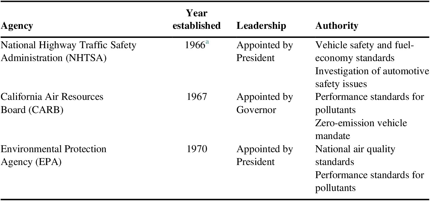
a Following a series of hearings regarding highway and vehicle safety, Congress created in 1966, among other agencies, the National Highway Safety Bureau (NHSB). In 1970, Congress established the National Highway Traffic Safety Administration (NHTSA) as a consolidation of the NHSB and other entities.
Despite the large body of published literature on automotive regulation, we find that conducting a BCA for low-income households is more challenging than commonly appreciated. We illustrate the analytic challenges for each type of automotive regulation and suggest an agenda for future research and regulatory analysis to overcome the challenges. The article is restricted to the automotive sector, but several of the key issues are equally applicable to health, safety and environmental regulations of the energy, food, and medical sectors.
To appreciate why the data systems of federal agencies do not routinely collect information on the income levels of affected citizens, it is useful to recall why the data systems were created in the first place. EPA’s pollution measurement system is a network of thousands of fixed monitoring devices around the country that are used to determine whether a state or region complies with the agency’s National Ambient Air Quality Standards (NAAQS) (EPA, 2021). Since the devices are fixed in location, they do not measure the exposures of specific individuals or households. Since the NAAQS are the same for households of all income levels, information on income is not relevant to determining compliance.
NHTSA administers two national data systems on motor vehicle crashes and injuries but neither collects information on the income levels of drivers or injured motorists (NHTSA, 2021). The Fatal Accident Reporting System (FARS) is a census of all motor vehicle crashes in the USA that lead to at least one fatality. The Crash Investigation Sampling System (CISS) collects data on a nationally representative sample of motor vehicle crashes where at least one vehicle is towed from the scene. It includes information on the level of severity of injuries experienced by occupants. Both FARS and CISS are designed to assist NHTSA engineers in devising the uniform Federal Motor Vehicle Safety Standards (FMVSSs) that are applicable to all new passenger vehicles sold in the USA. Since NHTSA is not authorized to establish different standards for different income groups, no information on income levels is collected routinely by the agency.
The article begins by exploring why the private automobile in the USA is critical to the well-being of low-income households. We then examine what is known about the benefits of automotive regulations for low-income households, followed by an assessment of the costs incurred by low-income households. The final section covers the future agenda for research and regulatory analysis.
1.1 The automobile and the poor
US Department of Health and Human Services reported that for the year 2021, the poverty guideline is $26,500 for a family of four (US DHHS, 2021). According to the U.S. Census Bureau, about 10.5% of people living in the USA – about 34 million people – are in households with reported incomes below the federal poverty line (Semega et al., Reference Semega, Kollar, Shrider and Creamer2020). Table 2 reveals that several sociodemographic characteristics predict elevated rates of poverty in the USA. After almost a decade of decline in the overall poverty rate, the COVID-19 recession induced another increase in poverty in the USA (Center on Budget and Policy Priorities, 2021).
Table 2 The rate of poverty in the USA, 2019, overall, and by group.

a Since the categories are partially overlapping, the entries in the first column do not add to the overall US total.
Among poor households, 20% do not own a car, 40% own one car, and another 40% own two or more (Pendall et al., Reference Pendall, Hayes, George and McDade2014). Access to a car increases the rate and duration of employment (Ong, Reference Ong2002; Baum, Reference Baum2009), boosts wages and earnings (Goldberg, Reference Goldberg2001; Raphael & Rice, Reference Raphael and Rice2002; Gurley & Bruce, Reference Gurley and Bruce2005; Ward & Savage, Reference Ward and Savage2007), reduces family reliance on public assistance (Ong, Reference Ong2002; Lucas & Nicholson, Reference Lucas and Nicholson2003), leads to improved educational opportunities and outcomes for children in the household (Bensinger, Reference Bensinger2011; Pendall et al., Reference Pendall, Hayes, George, Dawkins, Jeon, Knaap, Blumenberg, Pierce and Smart2015), improves use of health care services (Bensinger, Reference Bensinger2011), and enables families to relocate to safer neighborhoods (Badger, Reference Badger2014). Thus, access to a private automobile is crucial to anti-poverty efforts in the USA.
Public transit services in urban areas also play a vital role serving the needs of poor families. The percentage of trips by transit service is much higher among the very poor (15.9%) and marginally poor (8.2%) than it is among all other income groups in the USA (3–5%) (Mattson, Reference Mattson2012). Cities vary enormously in the quality and affordability of transit services, with the services in New York, Chicago, and San Francisco rated better than the services in Birmingham, Dallas, Detroit, Jackson, Riverside, and Provo (Tomer & Kane, Reference Tomer and Kane2014). Even where transit services are relatively good, they do not supply access to employment opportunities as effectively as the private automobile (Badger, Reference Badger2014). If a commute must be less than 90 minutes to sustain an employment relationship, transit services – given current routes and where the poor live – provide access to far fewer jobs for the urban poor than private vehicles do (Owen & Levinson, Reference Owen and Levinson2014; Tomer & Kane, Reference Tomer and Kane2014).
When a private automobile is acquired, it is likely to be new if the buyer is from the top 40% of USA income distribution or used if the buyer is from the bottom 40% (Pazzkiewicz, Reference Pazzkiewicz2003; Experian, 2008). Affordability of cars is a major concern. The average transaction price for a new vehicle in January 2021 was $40,857, compared to an all-time high of $25,410 for a used passenger vehicle in the second quarter of 2021 (Cox Automotive, 2021; Unrau, Reference Unrau2021). In comparison, average transactions prices in 2019 for new and used cars were $37,000 and $21,000, respectively; however, older used cars are purchased for as little as a few thousand dollars or less (Wagner, Reference Wagner2020). The vehicle purchase price is only the first facet of the total cost of ownership that includes interest payments on financing, taxes, registration and licensing fees, insurance payments and operating, maintenance, and repair expenses.
Poverty scholars suggest that a cost-effective strategy for the urban poor would be coordinated investments in upgraded local transit systems and subsidized access to ride sharing and private automobiles (Rubinar, Reference Rubinar2007; Pendall et al., Reference Pendall, Blumenberg and Dawkins2016). Thus, looking to the future, use of an automobile is crucial to the well-being of the poor. However, regulations of cars could complicate this strategy if they increase the cost of purchasing and/or using a car.
2 How federal automotive regulations benefit the poor
To clarify the offsetting factors impacting the regulatory benefits for low-income households, consider the simple equation:
 $$ Bi\hskip2pt =\hskip2pt Ri\times E\times Vi, $$
where Bi is the average benefit of a regulation for income class I, Ri is the baseline safety, health, or environmental risk within income class I, E is the average percentage effectiveness of the regulation in reducing risk, and Vi is the average willingness to pay (WTP) to reduce risk in income class i.
We focus specifically on the lower quintiles of the USA income distribution, when I = 1 or 2 out of 5. We assume that E is constant across income groups in long-term equilibrium (i.e., when all old vehicles have been replaced by new vehicles), and thus the variation in Bi will arise from variations in Ri and Vi. In the case of the elevated concentrations of pollutants inhaled by low-income populations (sometimes called intake fractions), we assume they are incorporated in Ri, and thus do not need to be captured in the engineering parameter E.
The environmental justice literature highlights that Ri is often concentrated in the bottom of the income distribution, especially among the poor. However, the distribution of Bi is also influenced by Vi, which is likely – due to constraints on ability to pay – to be relatively small in the bottom of the income distribution. Below we investigate the relative magnitudes of Ri and Vi but, as we shall explain, much more definitive research is necessary to clarify the relative magnitudes.
Note that, in practice, agencies typically make estimates of costs and benefits using an engineering approach that is not a function of household income or consumer WTP. In the case of federal fuel economy regulation, for example, NHTSA and EPA do not base benefit estimates on consumer WTP for fuel-economy improvement. The agencies simply make calculations of the projected savings in fuel-expenditures and implicitly assume that consumer WTP is equal to those savings.
2.1 Pollution from cars and light trucks
Over the last 50 years, the amount of pollution from cars and light trucks has declined dramatically. Despite steady growth in economic production and vehicle miles of travel, the average air concentrations of several primary and secondary pollutants declined sharply from 1970 to 2010 (U.S. EPA, 1997, 2011). A primary pollutant is emitted directly from the tailpipe, such as carbon monoxide, hydrocarbons and nitrogen oxides. A secondary pollutant, such as ozone, is formed in the atmosphere due to the interaction of primary pollutants with sunlight and other chemicals. Some pollutants are both primary and secondary pollutants (e.g., fine particulate matter, PM2.5). Before the Clean Air Act was adopted in 1970, automobiles were responsible for most of the air pollution in urban centers, at least for several primary pollutants. Even today, mobile sources – counting old and new heavy trucks as well as cars and light trucks – account for about 50% of NOx emissions, 30% of volatile organic compounds and 20% of direct particulate emissions (U.S. EPA, 2017b).
Tailpipe emissions of several primary pollutants are down 99% compared to pre-1970 emission rates (US U.S. EPA, 2017a). Much of the progress is attributable to the three-way catalytic converter but lead-free and low-sulfur gasoline, advanced fuel-injection systems, and on-board monitoring technologies have also played a crucial role.
EPA has taken considerable measures to accurately measure PM2.5 over the course of the last two decades. Both national and regional data collected show substantial declines in PM2.5 levels since 2000 as reflected by Table 3 below. There has been a steady rise in annual vehicle miles traveled from 1971 to 2019 – with periods of flattened growth or decline correlating to the oil price spikes of 1974, 1979, and 2008 – which makes an indirect case for emissions regulation in the automotive sector; even as vehicle miles traveled increases, regulation and innovation may be a highly effective avenue to reducing particulate matter pollution (Federal Highway Administration, 2020). Table 3 shows the largest declines in PM2.5 on the U.S. coastal regions and central regions (Figure 1).
Table 3 Decline in estimated black-white pollution gap by income quintile Change in PM2.5 level from 2000 to 2015.


Figure 1. PM2.5 air quality by U.S. region: 2000–2020, measured by concentration of PM2.5 in ug m−3. Source: Data sourced from EPA particulate matter (PM2.5) trends data on EPA.gov.
2.1.1 Exposures and health effects by income level
In cities that have experienced cleaner air, the health status of long-term residents has improved (Laden et al., Reference Laden, Schwartz, Speizer and Dockery2006; Peters et al., Reference Peters, Breitner, Cyrys, Stolzel, Pitz, Wolke, Heinrich, Kreyling, Kuchenhoff and Wichmann2009). From 1990 to 2010 alone, EPA estimates that the Clean Air Act programs averted 160,000 premature deaths from a common air pollutant, PM2.5, and 4,300 premature deaths from smog (U.S. EPA, 2011, 2018). The predominant clinical mechanism of action has been a decline in mortality from respiratory and cardiopulmonary diseases in older adults and infants.
Some scientists raise technical concerns about whether the causal relationship between community air pollution and premature mortality is established (Cox, Reference Cox2013; Boffetta et al., Reference Boffetta, Vecchia and Moolgavkar2015). Moreover, it is not easy to quantify the precise portion of the lifesaving that is attributable to cleaner cars and light trucks, since heavy trucks and stationary sources (e.g., electric utilities and manufacturing plants) emit some of the same pollutants as light-duty vehicles. The strongest evidence of health benefits from control of automotive pollution is for carbon monoxide and lead, since these two pollutants were emitted predominantly by mobile sources (Schwartz, Reference Schwartz1994; Currie & Neidell, Reference Currie and Neidell2005; Currie et al., Reference Currie, Neidell and Schmieder2009; Currie & Walker, Reference Currie and Walker2011).
With those research issues in mind, we explore to what extent low-income households have experienced health benefits due to clean air. From a scientific perspective, it would be ideal if large samples of low-income households had worn personal-exposure monitors during the period of clean air progress so that the magnitude of their exposure reductions could be quantified. Such information was not collected in the early years of the CARB and EPA programs, in part because fixed station monitors were used to determine community compliance with national air quality standards. Nonetheless, there are two lines of evidence suggesting that low-income households have been disproportionate beneficiaries.
First, within urban communities, low-income citizens breathe higher concentrations of air pollution than high-income households. The pattern has been shown in national studies using Census tract data and city-specific studies where residents in different communities are compared for air pollution exposure (Marshall et al., Reference Marshall, Granvold, Hoats, McKone, Deakin and Nazaroff2006; Bae et al., Reference Bae, Bassok and Kim2007; Bell & Ebisu, Reference Bell and Ebisu2012; Clark et al., Reference Clark, Millet and Marshall2014, Reference Clark, Millet and Marshall2017; Colmer et al., Reference Colmer, Hardman, Shimshack and Voorheis2020). The findings of these studies are plausible since low-income people are more likely to live near roadways and may have more direct inhalation exposure to primary pollution. It is less obvious how secondary pollution exposures vary by income status, as secondary pollution is formed and mixed over an entire region.
As illustrated by EPA data in Figure 2, wealthy Southern California residents can avoid regional ozone pollution by paying for higher-priced homes and apartments near the ocean. One study in southern California found that region-wide efforts to control ozone did disproportionately benefit low-income residents (Bae, Reference Bae2003). In other U.S. cities with elevated ozone levels, there may not be as much neighborhood-to-neighborhood variation in ozone levels.

Figure 2. EPA measurements of ozone and particulate matter in Southern California. Source: Visual obtained from EPA ozone and particulate matter interactive map at https://gispub.epa.gov/airnow; Ozone pollution is represented in orange, PM2.5 and PM10 pollution are represented in yellow.
One recent study found that the Black population, including low-income Black households, have experienced disproportionately large reductions in PM2.5 exposures since 2000. Table 3 demonstrates this effect. The authors explore several possible explanations for the decline and conclude that the implementation of the Clean Air Act is likely the predominant cause of the progress (Currie, Voorheis, and Walker, 2020).
Overall, the average gap in PM2.5 exposures between blacks and whites narrowed from 1.6 μg m−3 in 2000 to 0.5 μg m−3. Another study of California’s race statistics in comparison to PM2.5 exposure concluded that African Americans in the state are exposed to 43% higher PM2.5 pollution, Latino Californians 39%, than white Californians (Reichmuth, Reference Reichmuth2019). Table 3 indicates that the disproportionate clean air progress for blacks was experienced in all quintiles of the income distribution, including the lowest income quintile. The study did not consider the relative impacts of different rulemakings pursuant to the Clean Air Act and did not isolate the automotive contribution to PM2.5 levels.
Second, in addition to exposure differentials, low-income residents may be especially vulnerable to diseases caused or exacerbated by air pollution exposures (e.g., see Gouveia & Fletcher, Reference Gouveia and Fletcher2000; Health Effects Institute, 2000; Laurent et al., Reference Laurent, Bard, Laurent and Segala2007; Wong et al., Reference Wong, Kloog, Coul, Kosheleva, Zanobetti and Schwartz2016). Insofar as the poor have increased susceptibility to heart disease, cardiopulmonary disease, stroke or cancer, then the same amount of exposure reduction may reap more health benefit for a low-income person than a high-income person. There is evidence that the statistical association between air pollution and adverse health effects, including premature mortality, is larger among low-income people and African Americans than among higher-income residents and whites (Qian et al., Reference Qian, Dai, Wang, Zanobetti, Choirat and Schwartz2017).
In summary, the ideal scientific measurements have not been undertaken to determine whether the poor are disproportionate beneficiaries of automotive air pollution control. However, the indirect evidence on exposure differentials and public-health impacts suggests that the poor have gained substantially.
2.1.2 WTP for clean air by income level
According to BCA, the monetized benefits of clean air among the poor are derived using two concepts: consumer WTP and the value of statistical life (VSL). Low-income residents are viewed as “consumers” of clean air because they have to pay some of the bill for cleaner vehicles in the form of higher prices for vehicles, used or new; think upgraded technology such as catalytic converters and on-board monitoring systems. The VSL is the monetary value of saving one expected life with access to clean air. The valuation is not of an identified life – such as a trapped coal miner – but of a population-wide reduction in mortality probabilities sufficient to save one expected life (Viscusi & Masterman, Reference Viscusi and Masterman2017).
Determining the proper average VSL for low-income individuals is a difficult question that EPA and CARB have never analyzed and the Office of Management and Budget has not yet assigned them to analyze. To the best of our knowledge, environmental and health economists have never designed a study with the specific purpose of deriving a VSL value for the poor, certainly not one with a focus on air pollution risks.
EPA generally assumes that all beneficiaries of healthy air have the same VSL. In our case, the entire point of the article is to determine whether automotive regulations pass a restricted Kaldor-Hicks test for the low-income population. Thus, assuming a uniform VSL value for all income groups is not informative.
Lacking the ideal scientific information on WTP for clean air, one could start with a standard VSL value for the middle of the income distribution. Since VSL is expected to decline with income, one could adjust the standard VSL based on published estimates of the income elasticity of VSL. Viscusi and Masterman (Reference Viscusi and Masterman2017) surveyed the USA and international literatures on VSL and income, with most studies in the occupational safety setting. Their meta-analysis finds an average income elasticity of VSL within the USA of 0.5–0.7 and just above 1.0 outside the USA, where incomes tend to be lower.
For example, if the income elasticity value of 0.6 were a constant, then VSL would decline from $10 million for a $50,000 income to $7 million at $25,000 and to $5.4 million at $10,000. However, income elasticity is almost certainly not a constant; it presumably enlarges as income levels decline. After all, it seems doubtful that a person with an annual income of only $10,000 would be willing to pay $540 annually to avoid an incremental risk of death of 1 in 10,000 per year. That level of risk is an order-of-magnitude indication of the baseline level of risk people face from exposure to traffic crashes and PM2.5 air pollution. In contrast, as income rises the WTP for lifesaving becomes a smaller proportion of income but represents a higher absolute amount of money.
If income elasticity rises rapidly at low-income levels, then the average VSL for low-income Americans may be quite low, since payments for longevity enhancement compete with other basic necessities in life such as food, shelter and clothing. Exceptionally low-income households have virtually zero discretionary income once they have paid for the necessities of life. There is very little evidence on how low the VSL is for low-income households.
The best evidence we have found was reported by Kniesner et al. (Reference Kniesner, Viscusi and Ziliak2010) in the occupational context, where VSL values varied sharply by income level. Workers in the highest income group revealed VSL values that were a factor of 9 larger than workers in the lowest income group. The authors state: “The perceived economic benefits of risk regulation will be extremely low if income levels are low because the VSL declines at very low-income levels that is more than proportional to the decrease in income” (p. 28). Viscusi and Masterman (Reference Viscusi and Masterman2017) suggest that income elasticity for VSL may be as large as 2.0 toward the bottom of the wage distribution of USA workers, but VSL values for the working poor may be different than VSL values for the nonworking poor (e.g., the unemployed and disabled). More direct evidence is needed on the WTP of low-income households for clean air.
2.1.3 Summary on EPA/CARB standards
We conclude that it is not feasible, based on the available evidence, to determine what the monetized benefits of the EPA/CARB standards are for low-income populations. On one hand, the health benefits of clean air, in physiological terms, are likely to be disproportionately larger for low-income individuals because their exposures to automotive air pollution are relatively large and their physiological vulnerability to adverse health effects may be relatively large. On the other hand, their WTP for clean air, given their limited ability to pay, may be quite low, as reflected in income adjusted VSL values.
2.2 The safety of passenger vehicles
The National Highway Traffic Safety Administration (NHTSA), a unit of the U.S. Department of Transportation, was established in 1966 to establish FMVSSs covering everything from safety belts to center rear-mounted stop lamps (U.S. NHTSA, 2017). FMVSSs apply only to new vehicles; they affect older vehicles gradually as old vehicles are scrapped and replaced by new vehicles.
2.2.1 The safety impacts of NHTSA’s FMVSSs
NHTSA has published retrospective technology-effectiveness estimates for 82 specific safety technologies stimulated by the adoption of FMVSSs (appendix of Kahane, Reference Kahane2015). Those technologies include front disk brakes, electronic stability control systems, instrument panel upgrades, head-impact upgrades, improved door locks, lap and shoulder belts including belt pretensioners and load limiters, frontal airbags for both driver and passenger, adhesive windshield bonding, child safety seats, side door beams, curtain and side-impact airbags, roof crush resistant designs, rollover curtains and fuel-system integrity designs.
None of the lifesaving and injury-reducing estimates of these technologies address the impacts on low-income motorists. In fact, NHTSA’s data systems do not even collect information on the income levels of injured motorists. However, there is circumstantial evidence from academic studies that the safety benefits of NHTSA standards are enjoyed disproportionately by low-income motorists.
Cubbin and Smith (Reference Cubbin and Smith2002) analyzed peer-reviewed studies since 1960 that report associations between socioeconomic status (SES) of motorist and rates of fatal and nonfatal injury. Four of the five studies of fatal motor vehicle crash injuries found a negative association between SES and fatalities, and the one showing a positive association was restricted to youth in the Boston area. Braver (Reference Braver2003) found that known risky driving behaviors (i.e., those linked to fatalities) are concentrated among drivers with relatively low SES. She linked data on motor vehicle crashes to death certificates to discern level of education, race and ethnicity. The relative risks of crash death (per trip) were 1.48 for black men and 1.28 for Hispanic men compared to white men. The relative risks for black women were slightly elevated (1.19) but were not elevated for Hispanic women (0.99). The association of fatality risk with level of education of the driver was particularly large. The relative risks (per trip) for those who did not complete a high school education compared to those that completed at least some education beyond high school were quite large: 3.52 for men and 2.79 for women. The association of fatality risk per trip with low educational attainment was evident in all geographical locations: urban, suburban, small town and rural. Since level of education is highly correlated with income as reported by the U.S. Bureau of Labor Statistics (2017), we conclude that there is circumstantial – or indirect – evidence that low-income individuals experience a disproportionate share of the safety benefits of FMVSSs (Figure 3).

Figure 3. Income and educational attainment in 2019$. Source: Data based on historical income tables, Bureau of Labor Statistics Census Bureau, titled “Table A-3. Mean Earnings of Workers 18 Years and Over, by Educational Attainment, Race, Hispanic Origin, and Sex: 1975 to 2019.”
An important qualification is that the relative risks reported above are per trip. The number of trips may not be as large in low-income populations as high-income populations. The literature on vehicle miles of travel (VMT) generally shows a positive association between income and VMT, although VMT is a subtly different construct than number of trips. More research is necessary to determine whether, accounting for number of trips and VMT, low-income households experience a disproportionate share of the safety benefits of FMVSSs. Table 4 shows that low-income households (less than $20,000) per year engage in significantly fewer trips than households at higher-income levels.
Table 4 Annual person trips by motor vehicle per household, measured by household income, 2009.

2.2.2 WTP for vehicle safety by income level
Like was the case with clean air, there is a paucity of evidence on the WTP for safety among low-income motorists. We found only two studies, by the same researchers, and they concluded that WTP for auto safety features declines sharply as household income declines (Rohlfs et al., Reference Rohlfs, Sullivan and Kniesner2012, Reference Rohlfs, Sullivan and Kniesner2015). This finding is consistent with the pattern of introduction of automotive safety features in the auto industry: they generally start on the high-priced luxury models, and gradually penetrate the less expensive models over time.
2.2.3 Summary on NHTSA safety standards
We offer circumstantial or indirect evidence that the safety benefits of FMVSSs are experienced disproportionately by low-income motorists. However, this finding relies on measures of SES rather than income; nor does the evidence account for the number of trips or VMT by income level. Since WTP for vehicle safety is likely to fall sharply as income declines, we conclude that it cannot be determined whether the monetized benefits of NHTSA’s safety standards are disproportionately large or small among low-income households.
2.3 The fuel economy and greenhouse gas emissions of vehicles
NHTSA is responsible for fuel economy regulation while EPA and CARB regulate greenhouse gas (GHG) emissions from new passenger vehicles. Since fuel economy and GHG emissions are highly (and inversely) correlated, efforts have been made to harmonize the regulatory programs.
2.3.1 Benefits of fuel economy for the poor
The regulatory analyses by NHTSA and EPA find that the single largest category of benefits are private savings of fuel for motorists, a category of benefit that is much larger than the climate-related benefits. This finding was apparent in 2012 when the Obama administration used a substantial value for the social cost of carbon (SCC) and when the Trump administration used a much smaller SCC (US NHTSA, 2012; US U.S. EPA, 2012; U.S. EPA/CARB/NHTSA, 2016; U.S. EPA/NHTSA, 2020). Since climate change is likely to impact populations with limited ability to adapt to changing conditions, one should expect that low-income populations will incur a disproportionate share of the physical damages of climate change. However, even the most high-quality studies of climate damages do not report damage estimates for different income classes (e.g., see Hsiang et al., Reference Hsiang, Kopp, Jina, Rising, Delgado, Mohan and Rasmussen2017). As important as climate change is, were it not for the private fuel savings, it is questionable whether stringent fuel-economy or GHG standards would pass a strict benefit-cost test (Gayer & Viscusi, Reference Gayer and Viscusi2013).
Since the private fuel savings are crucial to the evaluation of fuel-economy and GHG standards, we examined how the fuel-saving benefits are experienced by low-income people. Greene and Welch (Reference Greene and Welch2017) provide one of the few cost-benefit analyses of automobile regulations that provide results by income class. They build a case that the fuel savings attributable to the 1980–2014 fuel-economy standards provide substantial gains to the poor. Low-income households rarely purchase new vehicles. As more fuel-efficient vehicles enter the used-car market, low-income households benefit from those vehicles. A key to their result is the fact that low-income households spend a higher percentage of their income on gasoline than high-income households. This leads them to conclude that federal fuel economy standards have a progressive impact.
It is ultimately feasible to disaggregate some of the benefits and costs of the federal fuel economy and GHG standards. Although the relevant regulatory impact analyses do not perform this disaggregation, our paper reviews two studies that present estimates of consumer savings in fuel expenditures by income group (National Research Council, 2015a; Greene & Welch, Reference Greene and Welch2017). Both studies conclude that the pattern of savings by income group is progressive, since low-income consumers spend a higher fraction of their income on automobile transport than high-income consumers. However, neither study address the distributional impacts of the environmental impacts of fuel-economy or GHG standards, in part because EPA does not collect the original information on pollution and GHG impacts that would be required to perform such disaggregation. We have not described the statistical methods used by the authors because they are available in the two references we cited.
2.3.2 Summary
Federal fuel economy standards and GHG standards are likely to benefit low-income households because they generate savings in fuel expenditures and they slow climate change, which inflicts damages on low-income households. However, we are unable to identify any studies of the SCC that are adjusted by income level. There is evidence that more fuel-efficient vehicles will benefit the poor, once new vehicles are sold in the used-vehicle market where low-income people access private vehicles.
2.4 Zero-emission vehicle requirements
The State of California and at least 10 aligned states have required that automakers earn sufficient zero-emission credits that a significant proportion of new vehicles will be zero emission by 2025 (CARB, 2017). The zero-emission vehicle (ZEV) requirement is expected to accelerate the commercialization of plug-in electric vehicles (PEV) and/or hydrogen fuel-cell electric vehicles (FCV). We consider here what the benefits of state ZEV regulations might be for low-income populations.
2.4.1 The benefits of state ZEV regulations for the poor
The original 1990 rationale for CARB’s ZEV program was to curb the atmospheric levels of smog and particulate matter pollution, especially in Los Angeles and the San Joaquin Valley. To the extent that the state ZEV requirements reduce smog and particulate matter levels, they will lead to health benefits for low-income populations. However, since 1990, CARB and EPA have issued regulations that have dramatically reduced (by more than 90%) the levels of pollution from gasoline-powered vehicles. Those regulated vehicles are certified for 150,000 miles of vehicle life, beyond the lifetime of the average passenger vehicle. Thus, the air quality advantages of a ZEV are much reduced today compared to what they were when the ZEV regulation was introduced in 1990.
Starting in 2009, CARB shifted the rationale for ZEV requirements to encompass GHG control as much as control of conventional pollutants. However, both EPA and CARB already have GHG performance standards for new passenger vehicles. When state regulations stimulate sales of PEVs and FCVs, they do not necessarily contribute to a net reduction in overall GHG emissions. Manufacturer compliance with state ZEV programs help manufacturers comply with CARB and EPA GHG standards. For each ZEV that a manufacturer sells, the manufacturer may offset that vehicle with one or more additional high-emitting vehicles due to the corporate-averaging provisions in GHG standards. Between 2018 and 2025, it seems likely that state ZEV programs will do more to shift GHG emissions around the USA than to reduce overall GHG emissions (Jenn et al., Reference Jenn, Azevedo and Michalek2016). Since the GHG standards do not account for the GHG emissions that ZEVs induce at the electric powerplant, it is possible that the state ZEV programs could induce a net increase in GHG emissions (National Research Council, 2015b).
There may be a long-run (post-2025) society-wide benefit of state-level ZEV programs since they stimulate technological innovation and diffusion. If PEVs and FCVs are commercially successful, it may be feasible to set stricter GHG standards post-2025 than would have been possible without the state-level ZEV programs.
2.4.2 Summary
Overall, we found no evidence that state-level ZEV programs would generate significant incremental health benefits for low-income populations, beyond those achieved by CARB and EPA performance standards. Insofar as the state ZEV programs benefit the poor, it may be through the used-car market since PEVs and FCVs have relatively low costs of operation (low fuel and maintenance/repair expenses). As PEVs and FCVs are sold to low-income buyers, they will enjoy the low cost of operating those vehicles, assuming that the original battery systems and electric motors last the entire life of the vehicle.
3 Do the poor pay any of the costs of federal automotive regulations?
When a regulation is imposed on a sector of the economy, the burdens of that regulation do not necessarily fall only on the regulated entities. By linking the tax-incidence literature in public economics to environmental policy, economists postulate that the distributional effects of a regulation vary based on market conditions: the extent of factor mobility, trade exposure, evasion, corruption, and imperfect competition (Fullerton & Muehlegger, Reference Fullerton and Muehlegger2019).
In this section, we examine the costs of federal auto regulations and how those costs might impact low-income households. Most of these costs are pecuniary in nature due to the addition of more expensive equipment to new vehicles but some regulations also have nonpecuniary impacts, both positive and negative, on valued features such as performance and safety.
In a larger conference paper that has informed this article, we estimated that the average incremental cost of production today – for all NHTSA, EPA, and CARB light-duty regulations – is in the vicinity of $6,000 to $7,000 per vehicle (for the 1967–2015 period). Table 5 summarizes the average incremental costs of vehicle regulation, stratified by type of regulation Since the average transactions cost for a new vehicle is approaching $40,000 per vehicle, it appears that the cumulative regulatory burden on new vehicles might be as large as 15–20% of the average transactions price of a new vehicle. Tear-down studies are necessary to estimate such costs precisely, since the costs of technologies may overlap, and engineers are constantly implementing innovations that minimize compliance costs.
Table 5 Per-vehicle cost additions 1967–2015 attributable to regulatory rules (NHTSA, EPA, DOT) in 2016$.

a Supplementary cost additions sourced from: Wang et al. (Reference Wang, Kling and Sperling1993) and Chen et al. (Reference Chen, Abeles and Sperling2004).
b Supplementary cost additions sourced from Greene and Welch (Reference Greene and Welch2017).
3.1 Who bears the costs of automotive regulations?
In theory, the cost burdens of automotive regulations could be borne by four distinct groups in the economy:
-
(i) Consumers of vehicles, if automakers pass on the costs to consumers in the form of higher vehicle prices or diminished product quality,
-
(ii) Employees in the industry, if firms respond to higher costs by reducing the compensation for employees or the number of employees,
-
(iii) Suppliers and/or dealers, through lower prices for their inputs and services, or
-
(iv) Owners/investors, if firms respond to higher costs by reducing returns to owners/investors (e.g., through diminished dividends to shareholders).
Under competitive market conditions, where all firms are subject to a regulatory burden, economic theory predicts that consumers will ultimately bear the costs of regulation. If instead the supply side of the vehicle market is oligopolistic, it is less obvious to what extent consumers will incur the cost burden (Fullerton & Heutel, Reference Fullerton and Heutel2010; Davis & Knittel, Reference Davis and Knittel2016; Muehlegger & Sweeney, Reference Muehlegger and Sweeney2017).
Forty years ago, the USA automotive industry was much more concentrated than it is today, and thus formal modeling was often done using oligopolistic assumptions (e.g., see Bresnahan, Reference Bresnahan1981; Berry et al., Reference Berry, Levinsohn and Pakes1995; Goldberg, Reference Goldberg1995, Reference Goldberg1998; Kleit, Reference Kleit2004). Due to the large post-1970 decline in GM’s market share and the rise of Asian imports and new startups – take Tesla, for example – the U.S. industry is much more competitive today than it was in 1970 (Cutcher-Gershenfeld et al., Reference Cutcher-Gershenfeld, Brooks and Mulloy2015; Davis & Knittel, Reference Davis and Knittel2016).
Prodigious literature examines how manufacturing firms handle changes in their input costs. Dornbusch (Reference Dornbusch1987) theorized that firms operating in competitive environments increase the amount of “pass through” to consumers as the proportion of the market exposed to the cost increase grows. Ashenfelter et al. (Reference Ashenfelter, Ashmore, Baker and McKernan1998) confirmed the theoretical prediction in their study of the office supply retail sector. A large stream of literature has confirmed the “pass through” hypothesis as it relates to the auto industry (e.g., Feenstra, Reference Feenstra1989; Knetter, Reference Knetter1989; Gagnon & Knetter, Reference Gagnon and Knetter1994; Goldberg, Reference Goldberg1995, Reference Goldberg1998; Feenstra et al., Reference Feenstra, Gagnon and Knetter1996; Goldberg & Knetter, Reference Goldberg and Knetter1997; Kleit, Reference Kleit2004). A common assumption is that production processes are constant returns to scale in the long-run and, under that assumption, consumers will ultimately bear the costs of business regulations under competitive market conditions.
Gron and Swenson (Reference Gron and Swenson2000) examined list prices of automobiles at the model level in the USA from 1984 to 1994 coupled with data on production, vehicle characteristics, foreign versus domestic firms, wages of employees, exchange rates, imported parts content, tariffs, and other variables. Their work rejects the hypothesis of 100% pass through to consumers, but they show that USA auto makers engage in greater pass-through pricing than Asian and European manufacturers, possibly due to the eagerness of importers to enlarge market share in lieu of recovering regulatory costs, at least in the short run (Dinopoulos & Kreinin, Reference Dinopoulos and Kreinin1988; Froot & Klemperer, Reference Froot and Klemperer1989).
Anderson and Sherwood (Reference Anderson and Sherwood2002) compared EPA’s ex ante estimates of regulatory costs to BLS-reported estimates of vehicle price changes for a bundle of EPA regulations adopted in the 1990s. They found that the actual price changes, calculated to be $350+ per vehicle in 2001 dollars are about $100 per vehicle smaller than ex ante estimates of vehicle costs (about $450 per vehicle). The discrepancy could be due to cost savings accomplished by industry or market constraints on pass-through pricing. There are also some limitations to the BLS price data, which cover only domestic vehicle manufacturers.
In a comparison of 1980–1967 model cars, Crandall et al. (Reference Crandall, Keeler and Lave1982) estimated the cumulative impact of federal emissions and safety regulations on the cost of owning and operating a vehicle. To control for increases in prices that would have occurred in the absence of regulation, they employ a series of price increases in the largely unregulated household appliance sector. They conclude that federal regulations increased the average cost of ownership of new vehicles by 18% over the study period.
Sperling et al. (Reference Sperling, Abeles, Bunch, Burke, Chen, Kurani and Turrentine2004) show that the average transactions price for a new vehicle grew steadily from $9,120 in 1967 to $21,600 in 2001 ($2001). They estimate that slightly less than 25% of this price increase is attributable to federal emissions and safety regulations. Much of the price increase is attributable to improvements in reliability, durability, fit and finish, power, accessories and other dimensions of quality. The term accessories includes a wide variety of important advances: air conditioning, power seat adjustments, power adjustable mirrors, and independent four-wheel suspension systems.
The consumer pass-through hypothesis is more tenable for federal emissions and safety regulations than it is for the early wave of federal fuel economy regulations (1975–2007). The original design of the Corporate Average Fuel Economy (CAFE) program made pass-through pricing difficult. All automakers, regardless of product mix, were subject to the same fuel-economy standard such as 27.5 miles per gallon for cars in model year 1990. In practice, those standards impacted only three high-volume manufacturers: GM, Ford and Chrysler, because the Big Three produced a higher proportion of large and performance-oriented vehicles than the Japanese vehicle makers. As a result, Toyota and Honda consistently met the standards without any incremental cost. In the 1975–2007 period, the Big Three were not able to pass on all of their compliance costs to consumers and thus experienced declines in profitability (Kleit, Reference Kleit1990, Reference Kleit2004; Jacobsen, Reference Jacobsen2013). When the federal fuel-economy standards were reformed in 2008 based on vehicle footprint, compliance costs were spread more evenly among automakers, although the overall societal efficiency of the standards was somewhat reduced (Ito & Sallee, Reference Ito and Sallee2018). It is likely that the footprint design of CAFE standards has facilitated pass-through pricing but more research on this question is needed.
Greene and Welch (Reference Greene and Welch2017) estimate the price impacts of federal fuel economy standards from 1975 to 2014, assuming that vehicle production costs are passed on to consumers of new vehicles and, later, to consumers of used vehicles. They estimated that the price impact could be as large as $2,310 to $3,850 per vehicle, or 27–42% of the observed vehicle-price increase over the period. The estimated price impacts are likely upper bounds since (a) some of the fuel-economy technologies would have been implemented without regulation (e.g., due to gasoline-price impacts), (b) some long-run cost savings are expected due to learning by doing and economies of scale, and (c) some of those costs were likely incurred by employees, suppliers and shareholders of the Big Three (rather than consumers) as the companies incurred losses, experienced layoffs and bankruptcy (Jacobsen, Reference Jacobsen2013).
3.2 Do regulations of new vehicles affect prices of used vehicles?
Since low-income households do not typically purchase new vehicles, they might seem insulated from the cost impact of federal regulations on new vehicles. The markets for new vehicles and old vehicles differ substantially in size and price range. The new vehicle market has been as large as 17 million vehicles per year, with prices ranging from less than $20,000 per vehicle to more than $100,000 per vehicle. The used vehicle market is typically over 30 million vehicles per year, with prices spanning an even larger range. The average transactions price of a used vehicle ($17,000) is less than half the price of the average new vehicle (Carley et al., Reference Carley, Duncan, Graham, Siddiki and Zirogiannis2017).
To perform regulatory cost analyses of how new vehicle regulations impact the poor, the relationships between the new- and used-vehicle markets need to be understood. However, we found a paucity of literature on how regulations of new vehicles influence the prices of used vehicles.
Theory suggests that rising prices for new vehicles should, over time, induce higher prices for used vehicles. Figure 4 illustrates this hypothesis from January 1995 period to January 2017. However, the consumer price index for used cars rose much more rapidly than new cars during the second half of the period.
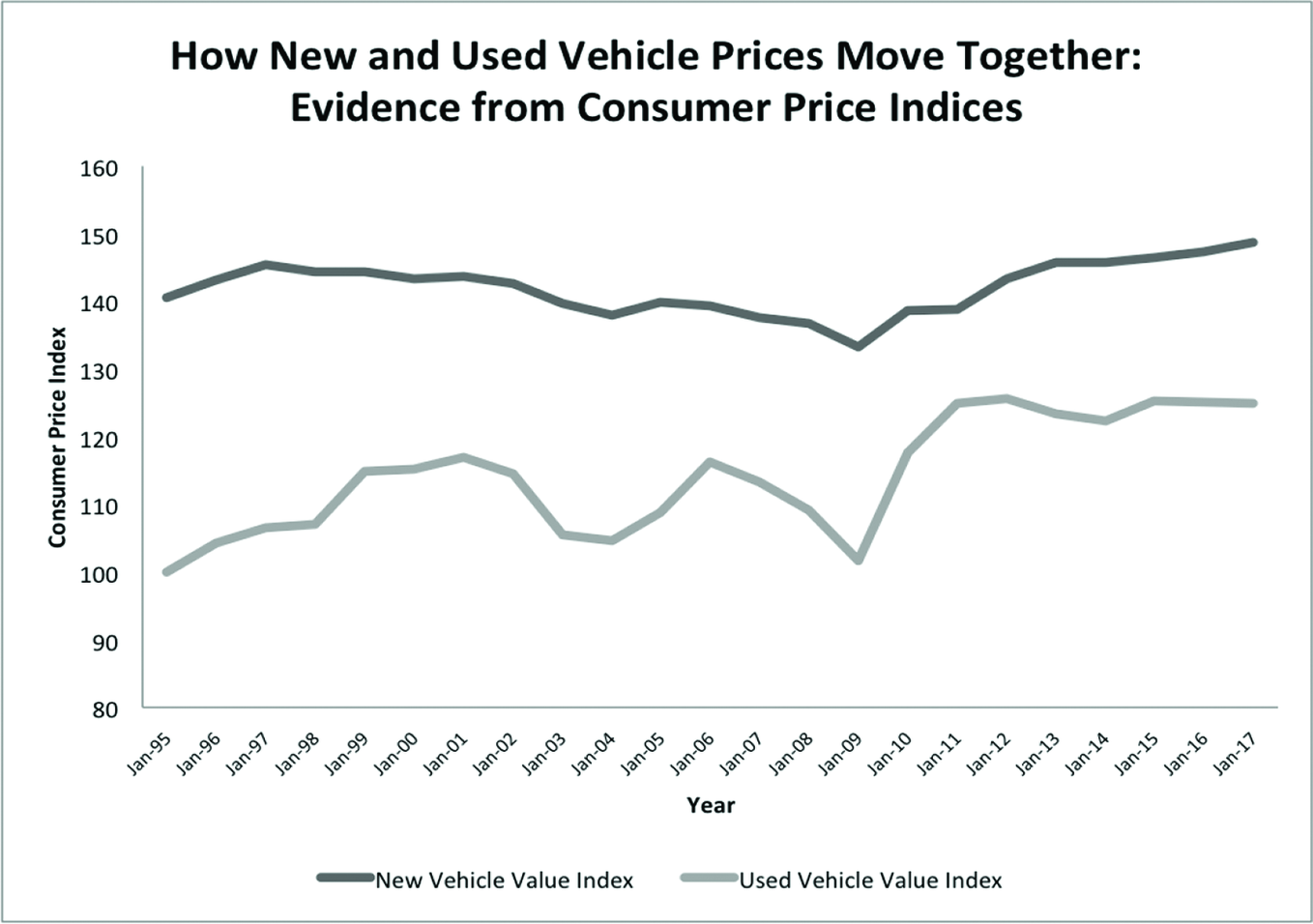
Figure 4. How new and used vehicle prices move together: evidence from consumer price indices. Source: Data sourced from the Bureau of Labor Statistics Consumer Price Indices.
The expectation of pass-through pricing from new vehicles to old vehicles arises from the fact that the used vehicle market is highly competitive and becoming more so as digital innovation is shaping the sales process. In addition to the large numbers of new car dealers who also sell used vehicles, there are large specialty companies dedicated to used cars such as Automation, CarMax, Carvana, and Shift. Moreover, any owner of a used car can choose to market their own vehicle, a dynamic that is completely different from the new vehicle market. Thus, suppliers of used vehicles will want to capture any of the depreciated value of a used vehicle as published by Kelley Blue Book, Edmunds and other sources. Depreciation is typically computed based on vehicle age and miles of travel, pegged at a fraction of the original vehicle purchase price. The prices offered by used vehicle markets presumably reflect the demand and supply of used vehicles.
In the short run, however, a used vehicle is a substitute for a new vehicle. Increases in new vehicle prices cause some consumers to enter the used vehicle market (or hold on to their existing vehicle longer) (Gruenspecht, Reference Gruenspecht1982). The price elasticity of demand for new vehicles is highly elastic in the short run, since consumers can hold on to their current vehicle a bit longer or buy a used vehicle instead, but the elasticity is larger in the long-run as consumers cannot hold on to old vehicles indefinitely (McAlinden et al., Reference McAlinden, Chen, Schultz and Andrea2016). Thus, higher new vehicle prices, whether due to regulation or other factors, create upward pressure on demand and prices for used vehicles (Gruenspecht, Reference Gruenspecht1982; Jacobsen, Reference Jacobsen2013; Jacobsen & van Bentham, Reference Jacobsen and van Bentham2015; Davis & Knittel, Reference Davis and Knittel2016).
When consumers demand more used vehicles, there is also a supply response in the used vehicle market, operating through the scrappage rate on older vehicles. Scrap rates increase gradually with vehicle age, from 1.6% for 2-year-old vehicles to 14.4% for 19-year-old vehicles (Jacobsen & van Bentham, Reference Jacobsen and van Bentham2015).
Consider the recurring dilemma faced by an owner of a used vehicle. Each time a vehicle breaks down, the owner must decide whether to repair and keep the vehicle, repair and sell the vehicle, or scrap the vehicle. Rational-choice theory predicts that he/she will choose to scrap it if and only if the prevailing price in the used vehicle market falls below the repair cost plus any residual value (Jacobsen & van Bentham, Reference Jacobsen and van Bentham2015). Thus, the markets and prices for new and used vehicles are linked through the scrappage rate.
3.2.1 Summary
Qualitatively, higher new vehicle prices are not good news for the poor due to pass-through pricing to old vehicles: about 80% of low-income households own and use passenger vehicles (Sawhill, Reference Sawhill2012). Over 60% of low-income workers commute alone to work each day by private vehicle (Hayes, Reference Hayes2008). Any factors that make used vehicles more expensive are thus likely to hurt the poor financially (Jacobsen, Reference Jacobsen2013; Davis & Knittel, Reference Davis and Knittel2016; Levinson, Reference Levinson2016).
We are aware of only one federal regulatory program (CAFE) that has been analyzed to determine whether the costs of regulation, as borne by the poor, are justified by the benefits of the program, as experienced by the poor. Both the National Research Council (2015a) and Greene and Welch (Reference Greene and Welch2017) present calculations suggesting that low-income motorists gain more from more fuel-efficient cars than they lose from the higher prices of cars with advanced fuel-efficiency technologies. The conclusions of both studies rest on very limited analysis of the impacts of new vehicle regulations on the prices of used vehicles. Nor did those studies examine the recent footprint-based reforms of the CAFE program, which may hurt the poor disproportionately because those reforms shift some compliance costs on to the smaller vehicles that the poor are likely to purchase (Levinson, Reference Levinson2016).
A related argument suggests that ZEV mandates might benefit the poor in the long-run, since electric cars have lower operating and repair costs than gasoline-powered cars (Bauer et al., Reference Bauer, Hsu and Lutsey2021). However, more study is needed to determine how many low-income households will use electric cars since they often lack a feasible place for home charging, they may be able to afford only one vehicle that must be capable of long-distance travel, and the price of electricity at public charging stations is much higher than private residential charging. Moreover, the repair-cost advantages of electric cars typically exclude the large replacement costs for batteries in the second half of an electric car’s life, the period when low-income households are most likely to own an electric car. More research is needed to determine how electric cars will impact the welfare of low-income households.
4 Conclusions and recommendations
The philosophical or moral premise of this article is that regulators should consider impacts on low-income Americans as well as the overall well-being of society. Low-income groups merit special consideration since they are not well organized for political action and are rarely among the loud voices heard from during federal rulemakings. We recognize that other groups in society may also merit consideration (e.g., racial minorities, small businesses and so forth) but most philosophical accounts of the need for equity in public policy would include the poor as one of the relevant groups for study.
In this article, we made a comprehensive assessment of available evidence to determine whether federal automotive regulations of pollution, safety and fuel economy accomplish more benefits than costs for the poor. A large body of evidence – direct and indirect – suggests that federal auto regulations have achieved significant benefits for low-income populations. However, the available evidence also suggests that low-income owners of vehicles pay higher prices for their vehicles due to federal regulations. We found remarkably little evidence concerning the relative magnitudes of costs and benefits of automotive regulation as experienced by low-income households.
The paucity is unlikely to be solved by creative analyses of existing data, though more effort in that direction is worth considering. EPA, CARB and NHTSA should address the paucity of information by including income data in their basic data systems. For EPA and CARB, some personal-exposure monitoring of pollutants by income status would be extremely useful; location of fixed station monitors in different income areas would also be useful. At NHTSA, the basic data on traffic injuries and fatalities should be augmented to include data on the income level of the motorist.
We also recommend that new federal rulemakings of the automotive sector include an information collection strategy to fill the gaps we have uncovered. If such data are collected, OMB could implement a special requirement that agencies estimate benefits and costs for low-income households in addition to the current society-wide BCA.
Specifically, each rulemaking should include a factual determination as to whether the rulemaking is likely to make the poor better off or worse off, using the preferences of the low-income population for evaluation purposes. If a proposed rulemaking appears to make low-income Americans worse off, the OMB should compel the agency to consider alternative regulatory designs that might have better outcomes for low-income households. In this analysis, we have not distinguished the rural poor from the urban poor, but automotive regulations may affect them differently. Automobile safety regulations may disproportionately benefit the rural poor because they take numerous car trips due to lack of public transit and the roads they travel may have many injury-producing crashes due to high speeds and older road designs, such as no division of traffic streams and poor markings of lanes. On the other hand, the rural poor may pay for catalytic converters and other air quality measures without experiencing the same degree of health benefit as the urban poor. We encourage future research with a focus on how the rural poor are impacted differently than the urban poor. We acknowledge that the equity analysis proposed here is much more limited than the comprehensive distributional analysis suggested by other scholars (e.g., see Adler & Posner, Reference Adler and Posner2006; Adler, Reference Adler2019).
Our discussion of poverty in this paper has treated poverty as a static construct even though individuals move in and out of poverty during a given year and over their lifetime. Episodic poverty, defined as poverty for two consecutive months within a 2-year period, was estimated at 27.5% for 2013–2014. Chronic poverty, defined as continuous poverty for two consecutive years, was estimated at only 6.4% for 2013–2014. Rates of chronic poverty were higher among women, children, Hispanic-Americans and African Americans (Mohanty, Reference Mohanty2019). The dynamic nature of poverty presents challenges for regulatory analysis with a focus on the poor. One option for analysts is to focus on the chronically poor. Another option is to cast a broader net and capture the episodically poor. However, as disaggregated measures of poverty are sought, it may be more difficult to finding matching information in the other aspects of the regulatory analysis.
As important as regulatory equity is, we acknowledge statutory constraints on efforts to protect the poor. We also note that regulatory reform for the poor may not always be a wise strategy. A well-developed literature shows the relative inefficiency of regulatory reform as a method of protecting the interests of low-income households compared to tax policy (e.g., see Hylland & Zeckhauser, Reference Hylland and Zeckhauser1979). Nonetheless, if politicians refuse to use tax policy for equity yet proceed with inequitable regulations, politicians might consider supplemental policies to advance or protect the interests of low-income households.
California is moving in this direction with its ZEV policies. The State now has income eligibility criteria for the consumer rebates offered after purchase of an electric car; special rebates are made available to low-income consumers. Also, the city of Los Angeles is using $1.6 million in state funding to place 100 all-electric and hybrid vehicles in low-income communities with a goal of serving 7,000 low-income households and removing 1,000 older gasoline-powered vehicles from the fleet. In the settlement of the lawsuit against Volkswagen concerning cheating on diesel emissions standards, the state of California insisted that VW make electric vehicle charging stations available in low-income communities. Such efforts are well intended, but some poverty scholars question whether public investments in electric cars are a cost-effective way to help the poor with their transportation needs (Pendall et al., Reference Pendall, Blumenberg and Dawkins2016).
The Biden administration is eager to bring more analysis of distributional equity into regulatory cost-benefit analysis, especially analysis of impacts on low-income, minority and marginalized groups. The Biden recommendations echo a call from the economics community in the 1930s, when Kaldor-Hicks efficiency was first advanced as a justification for BCA. Despite decades of intellectual interest in distributional equity analysis, analytic progress has been limited but the time seems ripe for further progress.
Acknowledgments
The authors thank L. Bennear, A. Finkel, J. German, B. Heim, M. Schultz, R. Keefe, J. Levy, T. Kniesner, K. Simon, P. Stevens, K. Viscusi, T. Walton, N. Zirogiannis, and K. Krutilla for helpful leads and suggestions of literature. Revisions to an initial draft were made in response to written comments from the following commissioned peer reviewers: J. Evans, A. Fraas, J. Hammitt, G. Helfand, and W. Wade. An earlier and longer version of the paper was commissioned by the Regulatory Studies Center at the University of Pennsylvania and presented at the 2018 Annual Meeting of the Society for Benefit-Cost Analysis. The conference paper, which is already available upon request through the University of Pennsylvania, will also be made available on the authors’ web site as soon as this paper is published.


 Open access