


1. Introduction
Due to recent advances in manufacturing technology, nanoparticles have become commercially available. One of the main applications is in the devices of thermal systems, where nanoparticles are dispersed in working fluids to improve the heat transfer efficiency, thanks to their outstanding features in terms of high thermal conductivity and large specific surface area. Suspensions of nanoparticles, known as nanofluids, have received considerable attention over the past decade in a variety of industrial applications, including electronics cooling, catalytic reactors and solar energy storage. The challenges and developments related to nanofluids can be referred to recent papers (Rashidi et al. Reference Rashidi, Eskandarian, Mahian and Poncet2019; Shah & Muhammad Reference Shah and Muhammad2019; Aglawe, Yadav & Thool Reference Aglawe, Yadav and Thool2021).
Despite their promising applications, the use of nanofluids does not always yield positive results. Some studies have pointed out that the addition of nanoparticles may present negative effects in practical applications. The reason is unclear since the mechanisms behind the heat and mass transfer are not fully understood. For example, it is well known that the enhanced heat transfer is not just caused by the improvement in the thermophysical properties of the fluids, and the efficiency of convective heat transfer may decrease when the volume fraction of nanoparticles exceeds a certain value (Keblinski et al. Reference Keblinski, Phillpot, Choi and Eastman2002; Keblinski, Prasher & Eapen Reference Keblinski, Prasher and Eapen2008; Ho et al. Reference Ho, Liu, Chang and Lin2010). Furthermore, it was found that the heat transfer rate is not only affected by the nanoparticle size, but also by the nanoparticle shape (Ghaziani & Hassanipour Reference Ghaziani and Hassanipour2017; Yazid, Sidik & Yahya Reference Yazid, Sidik and Yahya2017; Ambreen & Kim Reference Ambreen and Kim2020). Even so, the only fact could be verified is that the microscopic migration of nanoparticles plays a critical role in the determination of macroscopic heat and mass transport phenomena.
In terms of convective transport in nanofluids, the most widely used theory is the two-component mixture model proposed by Buongiorno (Reference Buongiorno2006). The theory regards nanoparticles as macromolecules dissolved in a base liquid, where the diffusion of nanoparticles is dominated by two microscopic slip mechanisms: thermophoresis and Brownian motion. Since Buongiorno's model was established, numerous researchers have employed it to explore the convective characteristics of various flow configurations via either theoretical analysis or numerical simulation. So far, however, there have not been any subtle experiments to validate his theory, and some measurements even apparently contradict it. For instance, most work on stability analysis shows that thermophoresis is a very strong destabilizing mechanism and always induces convection in nanofluids as long as they are heated from below (Tzou Reference Tzou2008a,Reference Tzoub; Kuznetsov & Nield Reference Kuznetsov and Nield2010; Nield & Kuznetsov Reference Nield and Kuznetsov2010; Ruo, Yan & Chang Reference Ruo, Yan and Chang2021). However, a recent experiment reported that the addition of nanoparticles can significantly improve the stability (Kumar, Sharma & Sood Reference Kumar, Sharma and Sood2020). On the other hand, some experiments pointed out that different shapes of nanoparticles affect the heat transfer efficiency (Elias et al. Reference Elias, Miqdad, Mahbubul, Saidur, Kamalisarvestani, Sohel, Hepbasli, Rahim and Amalina2013), which cannot be explained by the Buongiorno model.
Recently, Chang & Ruo (Reference Chang and Ruo2022) proposed a revised model to explain this contradiction by considering the particle settling effect due to gravity as the main diffusion mechanism. By performing the stability analysis for the Rayleigh–Bénard problem of nanofluids, they demonstrated that the gravity settling effect is a significant stabilizing mechanism that could suppress thermophoretic migration. In particular, they found that, for common nanofluids, the stability threshold should be determined by the relative strength of thermophoresis to the gravity settling effect.
This paper aims to extend the revised model to analyse the flow instability problem within a horizontal nanofluid-saturated porous medium layer heated from below. A porous medium is a solid material consisting of interconnected pores (voids). The utilization of porous media is a more promising technique than the conventional fins to enhance heat transfer efficiency. Due to the characteristics of high permeability and thermal conductivity, porous media such as metal foams have wide applications in various thermal devices such as electronic cooling, catalytic reactors and heat exchangers. The combination of a nanofluid and porous medium is regarded as an attractive technique in typical thermal systems due to its dramatic improvement of the heat transfer efficiency (Dukhan Reference Dukhan2023). For the latest developments in heat transfer in porous media with nanofluids the reader is referred to the review papers of Mahdi et al. (Reference Mahdi, Mohammed, Munisamy and Saeid2015) and Kasaeian et al. (Reference Kasaeian, Daneshazarian, Mahian, Koisi, Chamkha, Wongwises and Pop2017).
In nanofluid-saturated porous media, the interaction between nanoparticles, base fluid and the walls of the pores involves complex multiscale mechanisms, including microscopic particle migration, mesoscopic dispersion effects and macroscopic convective transport phenomena. It is indeed a big challenge to attempt to establish a continuum model that can properly describe the nonlinear interplay between the multiscale mechanisms in such a flow system. Most studies used a simple combination of the Darcy model and the Buongiorno model, and yielded a great number of informative results, as reviewed by Kasaeian et al. (Reference Kasaeian, Daneshazarian, Mahian, Koisi, Chamkha, Wongwises and Pop2017). A preliminary continuum model was proposed by Zhang, Li & Nakayama (Reference Zhang, Li and Nakayama2015) to consider the interaction between the nanoparticles and the walls of the pores, in which the volume average principle was used to take the effects of mechanical dispersion and local thermal non-equilibrium into account. However, this model has not yet been widely followed because some artificial coefficients are not easily obtained from experiments. This difficulty is not due to the modelling of nanoparticle migration but the theory of the porous medium itself.
Regarding general fluid flows in porous media, the theory has been developed for decades and numerous relevant studies can be found in the literature (Nield & Bejan Reference Nield and Bejan2017). However, there have been many new breakthroughs recently, one of which is the study of mechanical dispersion effects at the level of the pore scale. Two recent papers (Hewitt Reference Hewitt2020; De Paoli Reference De Paoli2023) have provided comprehensive reviews for the theoretical, numerical and experimental results in the field of convection in porous media, with more emphasis on nonlinear numerical simulations. Among these studies, the experiments conducted by Liang et al. (Reference Liang, Wen, Hesse and Dicarlo2018) showed that the strength of the dispersion effects mainly depends on the flow velocity and the configuration of the pores (e.g. geometry, porosity). When the flow velocity is low, all dispersion effects are ignorable and the Darcy model is appropriate to describe the convective transport phenomena. However, if the flow velocity is high enough, the mesoscopic dispersion effects will dominate the transport phenomena more than the microscopic molecular diffusion. The impact of dispersion effects on heat transfer performance has also been exhaustively explored via the nonlinear dynamic evolution, in which some interesting convection patterns, such as fingers (Hewitt, Neufeld & Lister Reference Hewitt, Neufeld and Lister2013; Liang et al. Reference Liang, Wen, Hesse and Dicarlo2018), proto-plumes and mega-plumes (Hewitt, Neufeld & Lister Reference Hewitt, Neufeld and Lister2014; Wen, Corson & Chini Reference Wen, Corson and Chini2015), were discovered.
The present study intends to explore the flow characteristics at the onset of instability from a quiescent state. Therefore, the mechanisms associated with high flow speeds such as mechanical dispersions can be ignored to simplify the analysis. The Darcy model was used to describe the convective transport behaviour in the porous medium layer. The assumption of local thermal equilibrium is made in which the interstitial heat transfer between the fluid and solid phase is negligible. The Buongiorno model is then employed to account for the migration of nanoparticles and the accompanying energy transport. However, we limited the analysis to the case of high porosity in order to ignore the interactions between the nanoparticles and the walls of the pores. As evidenced by molecular dynamics simulations (Michaelides Reference Michaelides2016, Reference Michaelides2017), the diffusion of nanoparticles adjacent to a solid boundary is actually slower than the diffusion far away from the wall, owing to the effect of hydraulic drag caused by the solid phase on the mobilities of the nanoparticles. If the pore size of the solid phase is not much larger than the nanoparticle size, the Brownian diffusion coefficient cannot be estimated simply by the existing formulas.
With some further assumptions, the resultant governing equations turn out to be basically the same as those in previous studies (Nield & Kuznetsov Reference Nield and Kuznetsov2009, Reference Nield and Kuznetsov2014; Ruo, Yan & Chang Reference Ruo, Yan and Chang2023), except for the additional term describing the gravity settling effect. Note that this settling effect is induced by the diffusion mechanism of nanoparticles due to gravity in the nanofluid, which is different from the effect of variable gravity considered in some previous studies (Yadav Reference Yadav2020; Yadav, Chu & Li Reference Yadav, Chu and Li2023). The objective of this study is to use the revised model to investigate the development and growth of the thermal instability of nanofluids in a horizontal porous medium layer, via linear stability analysis and direct numerical simulation. Hence, the physical mechanisms behind the onset of instability could be explored in a proper manner.
2. Modified convective transport equations
Consider a porous medium layer saturated by a nanofluid between two horizontal plates and heated from below with temperatures  $T_h$ and $T_c$ at $z=0$ and $z=H$, respectively (i.e. $T_h>T_c$). The nanofluid is a dilute suspension of nanoparticles with mean volume fraction $\phi _0$. It is assumed that the nanoparticles could stably suspend in the base fluid without the occurrence of aggregation or deposition, and the interaction between the nanoparticles and the walls of the pores could be neglected. The conservation equation of nanoparticles in the porous medium layer can be expressed by
 \begin{equation} \frac{\partial{\phi}}{\partial{t}}+\frac{1}{\varepsilon} \boldsymbol{v} \boldsymbol{\cdot} \boldsymbol{\nabla}{\phi} ={-} \frac{1}{\rho_p} \boldsymbol{\nabla}\boldsymbol{\cdot} \boldsymbol{J}_p, \end{equation}
where  $\varepsilon$ is the porosity of the porous medium, $\phi$ the volume fraction of nanoparticles, $\rho _p$ the density of nanoparticles, $\boldsymbol {v}$ the Darcy velocity and $\boldsymbol {J}_p$ the mass diffusion flux of nanoparticles. According to the revised model proposed by Chang & Ruo (Reference Chang and Ruo2022), the main slip mechanisms for the migration of nanoparticles should include the gravity settling effect in addition to thermophoresis and Brownian motion. Hence, $\boldsymbol {J}_p$ can be expressed by
 \begin{equation} \boldsymbol{J}_p= \boldsymbol{J}_{p,B} + \boldsymbol{J}_{p,T} + \boldsymbol{J}_{p,G} ={-}\rho_p D_B \boldsymbol{\nabla}{\phi} - \rho_p D_T \frac{\boldsymbol{\nabla}{T}}{T} + \rho_p \phi \boldsymbol{V}_g, \end{equation}
where  $T$ is the temperature, $\boldsymbol {V}_g$ the nanoparticle settling velocity due to gravity and $D_B$ and $D_T$ are the Brownian and thermophoretic diffusion coefficients, respectively. According to Buongiorno's work (Buongiorno Reference Buongiorno2006), they are defined as
 \begin{equation} \boldsymbol{V}_g =\frac{d^2_p (\rho_p- \rho_f) }{18 \mu_f} \boldsymbol{g}, \quad D_B = \frac{\kappa_B T}{3 {\rm \pi}d_p \mu_f},\quad D_T = \beta \frac{\mu_f}{\rho_f} \phi, \end{equation}
where  $\boldsymbol {g}$ is the gravitational acceleration, $d_p$ the nanoparticle diameter, $\kappa _B$ Boltzmann's constant, $\mu _f$ the viscosity of the base fluid, $\rho _f$ the fluid density and $\beta$ is the dimensionless thermophoretic diffusion coefficient, estimated by
 \begin{equation} \beta=0.26\frac{\kappa_f}{2\kappa_f+\kappa_p}, \end{equation}
in which  $\kappa _f$ and $\kappa _p$ are, respectively, the thermal conductivities of base fluid and nanoparticles. As discussed in the introduction, the present study considers a porous medium layer with high porosity, in which the effect of the hydraulic drag caused by the walls of the pores on the nanoparticle migration can be safely ignored. Thus, the diffusion coefficients may be estimated simply by those formulas used in an unbound fluid domain, i.e. (2.3a–c) and (2.4). Substituting (2.2) into (2.1) yields
 \begin{equation} \frac{\partial{\phi}}{\partial{t}}+\frac{1}{\varepsilon} \boldsymbol{v} \boldsymbol{\cdot} \boldsymbol{\nabla}{\phi} =\boldsymbol{\nabla}\boldsymbol{\cdot} \left( D_B \boldsymbol{\nabla}{\phi} + \beta \frac{\mu_f}{\rho_f} \frac{\phi \boldsymbol{\nabla}{T}}{T} - \phi \boldsymbol{V}_g \right). \end{equation}
The Darcy model is used for the porous medium and the momentum equation with the Boussinesq approximation takes the following form:
 \begin{equation} \boldsymbol{\nabla}{p} +\frac{\mu_f}{K} \boldsymbol{v} ={-} \{ \rho_p \phi +\rho_f (1 - \phi) [1-\beta_T (T-T_c)] \} g \boldsymbol{e}_z, \end{equation}
where  $p$ is the pressure, $\boldsymbol {e}_z$ the unit vector of the $z$-coordinate, $K$ the permeability and $\beta _T$ the thermal expansion coefficient. Because the fluid is quiescent before the onset of instability, we can assume that a local thermal equilibrium exists since the onset velocity is too low to induce interstitial heat transfer between the fluid and solid phases. For a discussion of the assumptions related to the local thermal non-equilibrium model the reader is referred to Zhang et al. (Reference Zhang, Li and Nakayama2015). Accordingly, the energy equation can be described by the following form:
 \begin{align} (\rho c)_m \frac{\partial{T}}{\partial{t}} + (\rho c)_f \boldsymbol{v} \boldsymbol{\cdot} \boldsymbol{\nabla}{T} = \kappa_m \nabla{^2}T+ \varepsilon (\rho c)_p \left( D_B \boldsymbol{\nabla}{\phi} + \beta \frac{\mu_f}{\rho_f} \frac{\phi \boldsymbol{\nabla}{T}}{T} - \phi \boldsymbol{V}_g \right)\boldsymbol{\cdot} \boldsymbol{\nabla}{T}, \end{align}
where  $c$ is the specific heat, and the subscripts ‘ $m$’, ‘ $f$’ and ‘ $p$’, respectively, denote the mean property of porous medium, fluid and nanoparticle. For example, the parameter $\kappa _m$, representing the effective thermal conductivity of the porous layer, is calculated by
 \begin{equation} \kappa_m=(1-\varepsilon) \kappa_s + \varepsilon \kappa_f, \end{equation}
where  $\kappa _s$ is the thermal conductivity of the solid phase of the porous medium. By assuming constant temperature and zero flux of nanoparticles at the impermeable boundaries, the boundary conditions at $z=0$ can be given by
 \begin{equation} w=0,\quad T=T_h,\quad D_B \frac{\partial{\phi}}{\partial{z}} + \beta \frac{\mu_f \phi} {\rho_f T} \frac{\partial{T}}{\partial{z}} + V_g \phi=0, \end{equation}
and at  $z=H$ we have
 \begin{equation} w=0,\quad T=T_c,\quad D_B \frac{\partial{\phi}}{\partial{z}} + \beta \frac{\mu_f \phi}{\rho_f T} \frac{\partial{T}}{\partial{z}} + V_g \phi=0, \end{equation}
where  $V_g=\|\boldsymbol {V}_g\|$ is the magnitude of the gravity settling velocity (Chang & Ruo Reference Chang and Ruo2022).
3. Linear stability analysis
3.1. Basic state solution
The dimensionless variables marked by asterisk are introduced as follows:
 \begin{equation} \left.\begin{gathered} (x^*,y^*,z^*)=\frac{(x,y,z)}{H},\quad t^*=\frac{\alpha_m}{H^2}t,\quad p^*=\frac{K}{\mu_f \alpha_m}p,\\ \boldsymbol{v}^*=\frac{H}{\alpha_m}\boldsymbol{v},\quad \phi^*=\frac{\phi}{\phi_0},\quad T^*=\frac{T-T_c}{T_h-T_c}, \end{gathered}\right\} \end{equation}
where  $\boldsymbol {v}^*=[u^*,v^*,w^*]$ and $\alpha _m=\kappa _m/(\rho c)_f$ represents the effective thermal diffusivity of the porous layer. Accordingly, the dimensionless governing equations together with the boundary conditions take the following forms:
 $$\begin{gather} \boldsymbol{\nabla}{^*} \boldsymbol{\cdot} \boldsymbol{v}^* =0, \end{gather}$$
 $$\begin{gather}\boldsymbol{\nabla}^* p^* + \boldsymbol{v}^* = (Ra_D T^* - Rm - Rn \phi^*) \boldsymbol{e}_z, \end{gather}$$
 $$\begin{gather}\frac{\partial \phi^*}{\partial t^*}+\frac{1}{\varepsilon} \boldsymbol{v}^* \boldsymbol{\cdot} \boldsymbol{\nabla}{^*} \phi^* = \frac{1}{Le} \boldsymbol{\nabla}{^*}\boldsymbol{\cdot} (\boldsymbol{\nabla}{^*} \phi^* +N_A \phi^* \boldsymbol{\nabla}{^*}T) + \frac{N_g}{Le} \frac{\partial \phi^*}{\partial z^*}, \end{gather}$$
 $$\begin{gather}\sigma\frac{\partial T^*}{\partial t^*}+ \boldsymbol{v}^* \boldsymbol{\cdot} \boldsymbol{\nabla}{^*} T^* = \nabla{^*}^2 T^* + \varepsilon \frac{N_B}{Le} (\boldsymbol{\nabla}{^*} \phi^* +N_A \phi^* \boldsymbol{\nabla}{^*}T^*) \boldsymbol{\cdot} \boldsymbol{\nabla}{^*} T^* + \varepsilon \frac{N_B N_g}{Le} \phi^* \frac{\partial T^*}{\partial z^*}, \end{gather}$$
 $$\begin{gather}w^*=0,\quad T^*=1,\quad \frac{\partial \phi^*}{\partial z^*} + N_A \phi^* \frac{\partial T^*}{\partial z^*}+ N_g \phi^*,\quad \mbox{at}\ z^*=0, \end{gather}$$
 $$\begin{gather}w^*=0,\quad T^*=0,\quad \frac{\partial \phi^*}{\partial z^*} + N_A \phi^* \frac{\partial T^*}{\partial z^*}+ N_g \phi^*,\quad \mbox{at}\ z^*=1. \end{gather}$$
The parameters in these equations are defined as
 \begin{align} \left.\begin{gathered} Ra_D= \frac{\rho_f \beta_T (T_h-T_c)KgH}{\mu_f \alpha_m},\quad Rm= \frac{\rho_f KgH}{\mu_f \alpha_m},\quad Rn= \frac{(\rho_p-\rho_f) \phi_0 KgH}{\mu_f \alpha_m},\\ Le= \frac{\alpha_m}{D_B},\quad N_A= \frac{\beta}{D_B}\frac{\mu_f}{\rho_f}\frac{T_h-T_c}{T_c}, \quad \sigma=\frac{(\rho c)_m}{(\rho c)_f}, \quad N_B=\frac{\rho_p c_p}{\rho_f c_f} \phi_0, \quad N_g=\frac{V_g H}{D_B}, \end{gathered}\right\} \end{align}
where  $Ra_D$ is the thermal Rayleigh–Darcy number, $Rm$ the density Rayleigh number and $Rn$ can be regarded as the concentration Rayleigh number. The parameter $Le$ is the Lewis number, which denotes the ratio of the effective thermal diffusivity to the Brownian diffusion coefficient, and $N_B$ represents the heat capacity ratio of nanoparticles to base fluid at a given mean nanoparticle concentration. The parameters $N_A$ and $N_g$ are the modified diffusivity ratios that respectively describe the effects of thermophoresis and gravity settling relative to Brownian motion at a specified nanoparticle diameter.
A time-independent quiescent solution of (3.2)–(3.7a–c) can be determined as the form of  $\boldsymbol {v}^* =0$, $\phi ^*=\bar {\phi }(z^*)$ and $T^*=\bar {T}(z^*)$. Consequently, (3.4) and (3.5) can be reduced to
 $$\begin{gather} \frac{\mbox{d}}{\mbox{d} z^*} \left(\frac{\mbox{d} \bar{\phi}}{\mbox{d} z^*} + N_A \bar{\phi} \frac{\mbox{d} \bar{T}}{\mbox{d} z^*}+ N_g \bar{\phi}\right)=0, \end{gather}$$
 $$\begin{gather}\frac{\mbox{d}^2 \bar{T}}{\mbox{d}^2 z^*} + \varepsilon \frac{N_B}{Le} \left( \frac{\mbox{d} \bar{\phi}}{\mbox{d} z^*} + N_A \bar{\phi} \frac{\mbox{d} \bar{T}}{\mbox{d} z^*} + N_g \bar{\phi} \right) \frac{\mbox{d}\bar{T}}{\mbox{d}z^*} =0. \end{gather}$$
Equation (3.9) can be integrated and, by employing the boundary conditions (3.6c) and (3.7c), we can obtain
 \begin{equation} \frac{\mbox{d} \bar{\phi}}{\mbox{d} z^*}+ N_A \bar{\phi} \frac{\mbox{d} \bar{T}}{\mbox{d} z^*} + N_g \bar{\phi}=0. \end{equation}
Equation (3.11) is then substituted into (3.10) to give
 \begin{equation} \bar{T} (z^*) =1-z^*, \end{equation}
and the general solution of  $\bar {\phi }$ can be derived by integrating (3.11) to give
 \begin{equation} \bar{\phi}(z^*) =C \exp(N_E z^*), \end{equation}
in which the parameter  $N_E$ is defined as $N_E= N_A-N_g$. The coefficient C can be determined by integrating $\bar {\phi }$ across the porous layer and the integration should be equal to unity due to the conservation of the nanoparticle concentration. Accordingly, the base-state solution of $\bar {\phi }$ can be obtained and written as
 \begin{equation} \bar{\phi}(z^*) = \frac{N_E \exp(N_E z^*)}{\exp(N_E)-1}. \end{equation}
Obviously,  $\bar {\phi }$ is a nonlinear function of $z^*$ and depends heavily on the parameter $N_E$. The profiles of $\bar {\phi }$ across the porous medium layer for several assigned values of $N_E$ are shown in figure 1. This solution is basically the same as that of the nanoparticle concentration in the thermal instability problem of a horizontal nanofluid layer (Chang & Ruo Reference Chang and Ruo2022).

Figure 1. The profiles of normalized nanoparticle volume fraction across the porous layer before the onset of convection.
3.2. Linearization and normal mode expansion
To perform the linear stability analysis, small perturbations are superimposed on the base-state solution to give the form
 \begin{align} \boldsymbol{v}^*= \boldsymbol{v}^{\prime} = [u^{\prime}, v^{\prime}, w^{\prime}], \quad \phi^*= \bar{\phi}(z^*)+ \phi^{\prime}, \quad T^*= \bar{T}(z^*)+ T^{\prime}, \quad p^*= \bar{p}(z^*)+ p^{\prime}. \end{align}
Equations (3.2)–(3.7a–c) can be linearized accordingly by neglecting high-order terms to give
 $$\begin{gather} \boldsymbol{\nabla} \boldsymbol{\cdot} \boldsymbol{v}^{\prime} =0, \end{gather}$$
 $$\begin{gather}0={-}\boldsymbol{\nabla}^* p^{\prime} - \boldsymbol{v}^{\prime} + (Ra_D T^{\prime} - Rn \phi^{\prime}) \boldsymbol{e}_z, \end{gather}$$
 $$\begin{gather}\frac{\partial \phi^{\prime}}{\partial t^*}+\frac{1}{\varepsilon} N_E\bar{\phi}w^{\prime} = \frac{1}{Le} \left[\nabla{^{*2}} \phi^{\prime} +N_A\left(\bar{\phi} \nabla^{*2} T^{\prime} -\frac{\partial{\phi^{\prime}}}{\partial{z}^*}+ N_E \bar{\phi} \frac{\partial{T^{\prime}}}{\partial{z}^*}\right) + N_g\frac{\partial \phi^{\prime}}{\partial z^*}\right], \end{gather}$$
 \begin{gather} \sigma\frac{\partial T^{\prime}}{\partial t^*} -w^{\prime} = \nabla^{*2} T^{\prime} + \varepsilon \frac{N_B}{Le} \left(N_E \bar{\phi} \frac{\partial{T^{\prime}}}{\partial{z}^*} -\frac{\partial{\phi^{\prime}}}{\partial{z}^*}\right) \nonumber\\ +\,\varepsilon \frac{N_A N_B}{Le} \left(\phi^{\prime}- 2\bar{\phi} \frac{\partial{T^{\prime}}}{\partial{z}^*}\right) + \varepsilon \frac{N_B N_g}{Le} \left(\bar{\phi} \frac{\partial{T^{\prime}}}{\partial{z}^*} + \frac{\mbox{d} \bar{T}}{\mbox{d}z^*}\phi^{\prime}\right), \end{gather}
and the boundary conditions at  $z^*=0$ and $z^*=1$ are
 \begin{equation} w^{\prime}=0, \quad T^{\prime}=0,\quad \frac{\partial \phi^{\prime}}{\partial z^*} + N_A \bar{\phi} \frac{\partial T^{\prime}}{\partial z^*}- N_E \phi^{\prime} =0 . \end{equation}
By taking the curl twice on (3.17), the pressure term can be eliminated and the  $z$-component leads to
 \begin{equation} \nabla^{*2} w^{\prime} = Ra_D \left(\frac{\partial^2 T^{\prime}}{\partial x^{*2}} +\frac{\partial^2 T^{\prime}}{\partial y^{*2}}\right) - Rn \left(\frac{\partial^2 \phi^{\prime}}{\partial x^{*2}} +\frac{\partial^2 \phi^{\prime}}{\partial y^{*2}}\right). \end{equation}
The differential equations (3.18), (3.19) and (3.21) together with the boundary conditions (3.20a–c) establish a boundary value problem. Normal modes are employed to expand the small perturbations in the following form:
 \begin{equation} [w^{\prime}, T^{\prime}, \phi^{\prime}]=[\hat{w}(z^*),\hat{T}(z^*),\hat{\phi}(z^*)] \exp (st^*+ \mbox{i}k_x x^* + \mbox{i} k_y y^*), \end{equation}
where  $k_x$ and $k_y$ are the wavenumbers in the x and y directions, respectively, and $s=s_r+\mbox {i}s_i$ is a complex number in which the real part $s_r$ accounts for the growth rate of disturbance and the imaginary part $s_i$ is the oscillatory frequency. The neutral state is determined by the condition of $s_r=0$. Substituting (3.22) into the governing equations, we can obtain
 $$\begin{gather} \frac{N_E}{\varepsilon} \bar{\phi} \hat{w} - \frac{N_A \bar{\phi}}{Le} (D^2 - k^2 + N_ED) \hat{T} - \frac{1}{Le} (D^2 - k^2 - N_ED) \hat{\phi}={-}s \hat{\phi}, \end{gather}$$
 $$\begin{gather}\hat{w} + \left(D^2-k^2-\varepsilon \frac{N_A N_B}{Le}\bar{\phi}D\right) \hat{T} -\varepsilon \frac{N_B}{Le} (D-N_E) \hat{\phi} =s \sigma \hat{T}, \end{gather}$$
 $$\begin{gather}(D^2-k^2) \hat{w} + k^2 (Ra_D \hat{T} - Rn \hat{\phi} )=0, \end{gather}$$
and the boundary conditions at  $z^*=0$ and $z^*=1$ are
 \begin{equation} \hat{w}=0,\quad \hat{T}=0,\quad D\hat{\phi}+ N_A \bar{\phi} D \hat{T} -N_E \hat{\phi} =0. \end{equation}
Here,  $D\equiv \textrm {d}/\textrm {d} z^*$ and $k=\sqrt {k^2_x+k^2_y}$ is defined as the horizontal wavenumber. Equations (3.23)–(3.26a–c) form an eigenvalue problem that could be solved by the Chebyshev collocation method. Firstly, the coordinate $z^*$ is transformed into the domain of $\xi$ by the relationship $z^*=(\xi +1)/2$. Thus, the variable $\xi$ is defined within the domain of $-1 \le \xi \le 1$, and then M-terms of the Chebyshev polynomials are employed as the set of base functions to expand each of the variables as follows:
 \begin{align} \hat{w}(\xi_j) \cong \sum_{m=0}^{M} a_{wm} \varPsi_m (\xi_j), \quad \hat{T}(\xi_j) \cong \sum_{m=0}^{M} a_{Tm} \varPsi_m (\xi_j), \quad \hat{\phi}(\xi_j) \cong \sum_{m=0}^{M} a_{\phi m} \varPsi_m (\xi_j), \end{align}
where  $\varPsi _m (\xi _j)=\cos {(m\cos {^{-1} \xi _j})}.$ These expansions should satisfy not only the system equations at the interior collocated points $\xi _j= \cos {(j {\rm \pi}/M)}$ with $j=1,2\cdots (M-1)$, but also the boundary conditions at $\xi =\pm 1$. Accordingly, we can obtain a matrix equation as the following form:
 \begin{equation} \boldsymbol{\mathsf{A}} \boldsymbol{U}= s \boldsymbol{\mathsf{B}} \boldsymbol{U}, \end{equation}
where  $\boldsymbol {U}=\{\hat {w}(\xi _0),\ldots \hat {w}(\xi _M),\hat {T}(\xi _0),\ldots \hat {T}(\xi _M),\hat {\phi }(\xi _0),\ldots \hat {\phi }(\xi _M)\} \in R^{3M+3}$ and $\boldsymbol{\mathsf{A}}$ and $\boldsymbol{\mathsf{B}}$ are the coefficient matrices. A matrix algorithm was used to calculate the eigenvalues and one can get sufficient precision for the numerical solution with $M=30$. The detailed procedure for implementing the calculation can be found in Boyd (Reference Boyd1989) and Canuto et al. (Reference Canuto, Hussaini, Quarteroni and Zang2007).
4. Numerical scheme for nonlinear dynamic simulation
For numerical simulation, the Chebyshev collocation method with multi-domain decomposition (Canuto et al. Reference Canuto, Hussaini, Quarteroni and Zang2007) was used to discretize the governing equations (3.2)–(3.7a–c), in a two-dimensional rectangular domain with aspect ratio  $a_r$, which is defined as the ratio of width to height. This numerical approach is implemented by partitioning the flow field into multiple subdomains. Within each subdomain, only a few collocated points (i.e. Chebyshev–Gauss–Lobatto grid) are specified in order to suppress the possible contamination of high-frequency modes. In this way, the continuity condition of the physical field must be imposed at the interface between the subdomains. In the present simulations with $a_r=6$, we typically used 15–90 subdomains with 5 collocated points in both the $x$ and $y$ directions in each subdomain. The subdomains are somewhat similar to the grids used in local approximation methods such as the finite element method. Therefore, the average distance of collocated points within a subdomain can be equivalently regarded as the resolution of the grid system. Note that the location of the collocated point is where the physical quantities are stored.
To perform the computation efficiently and enforce the continuity equation, we adopt the streamfunction  $\psi$ to replace the velocity. The momentum equation (3.3) becomes
 \begin{equation} \nabla^{*2} \psi -Ra_D \frac{\partial T^*}{\partial x^*} +Rn \frac{\partial \phi^*}{\partial x^*} =0. \end{equation}
A typical difficulty related to the numerical simulation of nanofluid flow is that the Lewis number is generally very large, which is due to the time scale of thermal diffusion being much shorter than that of Brownian diffusion. This feature inevitably causes a numerical instability when a high spatial gradient of concentration develops as time evolves. To improve numerical stability, we change (3.4) into the conservation form
 \begin{equation} \frac{\partial \phi^*}{\partial t^*}={-}\boldsymbol{\nabla}^* \boldsymbol{\cdot} \boldsymbol{Q}_c, \end{equation}
where  $\boldsymbol {Q}_c$ denotes the dimensionless nanoparticles flux through an infinitesimal control volume, given by
 \begin{equation} \boldsymbol{Q}_c= \frac{1}{\varepsilon} \phi^* \boldsymbol{v}^* - \frac{1}{Le} (\boldsymbol{\nabla}^* \phi^* + N_A \phi^* \boldsymbol{\nabla}^* T^* + N_g \phi^* \boldsymbol{e}_z). \end{equation}
Accordingly, we can advance the time evolution of concentration explicitly with a second-order Adams–Bashforth scheme. Such a treatment can suppress the numerical instability induced by the stiffness of the matrix obtained by implicitly discretizing the diffusion term.
For the other equations, the linear and nonlinear transport terms are treated explicitly and implicitly, respectively. Then, they are solved together with the following boundary conditions:
 $$\begin{gather} \psi=0,\quad \frac{\partial T^*}{\partial x^*}=0,\quad \frac{\partial \phi^*}{\partial x^*}=0,\quad \mbox{at}\ x^*=0\ \mbox{and}\ a_r, \end{gather}$$
 $$\begin{gather}\psi=0,\quad T^*=1,\quad \frac{\partial \phi^*}{\partial z^*} +N_A \phi^* \frac{\partial T^*}{\partial z^*} + N_g \phi^*=0,\quad \mbox{at}\ z^*=0, \end{gather}$$
 $$\begin{gather}\psi=0,\quad T^*=0,\quad \frac{\partial \phi^*}{\partial z^*} +N_A \phi^* \frac{\partial T^*}{\partial z^*} + N_g \phi^*=0,\quad \mbox{at}\ z^*=1. \end{gather}$$
Obviously, some of the boundary conditions are not of the type of Dirichlet. Therefore, we treat the nonlinear terms implicitly and the linear terms explicitly. In the simulations, we advance all the dynamic equations in time and automatically adjust the size of time step according to the Courant–Friedrichs–Lewy (CFL) condition, where the smallest Chebyshev–Gauss–Lobatto grid is considered as the mesh size.
5. Results and discussion
The numerical code was first verified by making a comparison of the results with the limiting case that the nanoparticle volume fraction  $\phi _0$ is set to zero. That is, the system reduces to the conventional thermal convection problem of a horizontal porous layer saturated by a general viscous fluid, which is named the Horton-Rogers–Lapwood problem (Nield & Bejan Reference Nield and Bejan2017). It is well known that the theoretical values of the critical Rayleigh–Darcy number $Ra_{D,c}$ and the corresponding critical wavenumber $k_c$ are $4{\rm \pi} ^2$ and ${\rm \pi}$, respectively. The present numerical results are the same exactly as those of the Horton-Rogers–Lapwood problem. To perform the analysis for a nanofluid, the parameters used in the analyses are based on a Al $_2$O
$_2$O $_3/$water nanofluid in a metal foam of aluminium, which can be found in the experimental study of Ghaziani & Hassanipour (Reference Ghaziani and Hassanipour2017). The corresponding thermophysical properties are listed in table 1. Notice that the porosity and permeability are based on experimental data which are not correlated by the Kozeny–Carman correlation and we can obtain $\beta = 3.85\times 10^{-3}$ and $\alpha _m = 4.68\times 10^{-6}$ m $^2$ s $^{-1}$ according to (2.4) and (2.8), respectively. Then, the dimensionless parameters defined in (3.8a–h) can be determined for a given porous layer thickness $H$ and a specified mean diameter of nanoparticles $d_p$.
Table 1. Thermophysical properties used in the present analysis at room temperature.

Note that both  $Ra_D$ and $N_A$ depend on the temperature difference ${\rm \Delta} T$ (i.e. ${\rm \Delta} T=T_h-T_c$). Therefore, they can be correlated by
 \begin{equation} \chi_A= \frac{Ra_D}{N_A} = \frac{\rho^2_f \beta_T D_B T_c KHg}{\mu^2_f \alpha_m \beta}. \end{equation}
Similarly, the parameters  $Rn$ and $N_B$ are dependent on $\phi _0$ and they can be linked by
 \begin{equation} \chi_B= \frac{Rn}{N_B} = \frac{(\rho_p-\rho_f) \rho_f c_f KHg}{\mu_f \alpha_m \rho_p c_p}. \end{equation}
The stability characteristics would be explored by considering nanoparticles with different sizes of the mean diameter  $d_p$ to evaluate the influence of gravity settling. Three typical diameters: 20, 40 and 60 nm, will be employed, which stand for the small, moderate and large sizes of nanoparticles, respectively. The following sections will discuss the results in sequence.
5.1. Results of nanofluid with small-diameter nanoparticles
The case of the nanofluid containing small-size nanoparticles was examined first with  $d_p=20$ nm and $H=0.05$ m. The corresponding dimensionless parameters are $Le = 1.91\times 10^5$, $N_g=1.39$, $\chi _A=4.99$ and $\chi _B=40\,916$. The concentration Rayleigh number $Rn$ indicates the effect of nanoparticle volume fraction as the definition in (3.8c). The variation of neutral curves for several selected values of $Rn$ is illustrated in figure 2. The curve of $Rn =0$ corresponds to $\phi _0=0$, which is the same as that of general viscous fluids with the minimum located at $Ra_{D,c}=4{\rm \pi} ^2 ({\sim }39.47)$ and $k_c={\rm \pi} ({\sim }3.14)$. The corresponding temperature difference across the porous layer ${\rm \Delta} T$ is 16.87 K. It is found that the neutral curve descends quickly with increasing $Rn$ and the minimum on the curve moves to the left rapidly. For the curve of $Rn=5\times 10^{-5}$, which is equivalent to $\phi _0 =1.52\times 10^{-9}$, the critical Rayleigh–Darcy number $Ra_{D,c}$ and critical wavenumber $k_c$ reduce to 12.71 and 1.22, respectively. As $Rn$ increases to $10^{-4}$, $Ra_{D,c}$ reduces further to 9.85 and $k_c$ approaches zero, which corresponds to $\phi _0 =3.04\times 10^{-9}$ and ${\rm \Delta} T=4.21$ K. This result reveals that the addition of nanoparticles to the base fluid exerts a vigorous destabilizing effect on the system. Once $Rn$ increases further (i.e. $Rn>10^{-3}$), the neutral curve tends to be a horizontal line and the critical Rayleigh number remains constant at 6.94.

Figure 2. Neutral curves of several assigned values of  $Rn$ for $d_p=20$ nm.
To further manifest the instability characteristics, we demonstrate the variations of  $Ra_{D,c}$ and $k_c$ with $Rn$ respectively in figures 3(a) and 3(b). The case of ignoring the effect of gravity settling with $N_g=0$ is also shown for comparison. For the case $N_g=1.39$, one can see that $Ra_{D,c}$ declines rapidly when $Rn$ increases and then approaches a constant 6.94 as $Rn>10^{-3}$, which renders $N_E \rightarrow 0$ or $N_A \rightarrow N_g$. The corresponding critical wavenumber $k_c$ also experiences an abrupt decline and tends to be zero after $Rn>10^{-4}$, while it begins to rise from zero as $Rn>1$. Note that the neutral curve for the case with $Rn > 1$ still exhibits a near horizontal line, as shown in figure 2, but the critical point moves to the right gradually as $Rn$ increases. For the case $N_g=0$ in the absence of gravity settling effect, however, both $Ra_{D,c}$ and $k_c$ reduce to zero eventually as $Rn$ increases, which indicates an unrealistically unconditionally unstable system. The difference in the predictions of instability behaviours verifies that the effect of the gravity settling of the nanoparticles plays an important role in the flow instability analysis of nanofluids. Figure 4 illustrates the three typical patterns of convection cells after $Rn$ exceeds 1. As shown in figure 4(a) for $Rn = 2.5$, the convection cells appear with larger wavelength and the gradient of the streamfunction is significant in the regions adjacent to the upper and lower boundaries. As $Rn$ increases to 25, as in figure 4(b), the wavelength is shortened and the convection magnitude is distributed uniformly across the porous layer. The wavelength decreases further as $Rn$ increases to 250, as shown in figure 4(c). The convection gradually concentrates within the central part of the porous layer, with more vigorous flow indicated by the steep gradient of the streamfunction. Note that all these cases belong to the stationary mode. According to (2.3c), the thermophoretic diffusivity is proportional to the volume fraction of nanoparticles. Hence, the instability characteristic reveals that an increase in the effect of thermophoresis would shorten the wavelength and enhance the convection at the onset of instability once the nanoparticle concentration exceeds a certain critical value.

Figure 3. Variations of (a) the critical Rayleigh number  $Ra_{D,c}$ and (b) the critical wavenumber $k_c$ with $Rn$ for the case of $d_p=20$ nm.

Figure 4. The flow patterns of onset convection cells for  $d_p=20$ nm: (a) $Rn = 2.5$ and $k_c=0.649$, (b) $Rn = 25$ and $k_c=3.214$ and (c) $Rn = 250$ and $k_c=5.971$.
Although the physical mechanisms dominating the instability behaviours can be revealed by the linear stability analysis, most conditions in practical engineering applications occur in the nonlinear region. For example, the Rayleigh–Darcy number would be 23.35 for a nanofluid with a nanoparticle volume fraction of 0.076 % (i.e.  $Rn = 25$) and temperature difference of 10 K across the porous layer, which is much greater than the critical value 6.94 predicted by the linear stability analysis. It is reasonable to expect the convection would be more vigorous and the instability modes would be coupled together to evolve and grow dynamically with time.
In order to explore the flow characteristics after the onset of instability, the spectrum of the growth rate of small disturbances was investigated and the flow evolution was simulated by direct numerical simulation. Figure 5 displays the spectrum of the growth rate  $s_r$ with wavenumber $k$ for three typical values of $Ra_D$ at $Rn = 25$ with $d_p=20$ nm. As $Ra_D=6.95$, which is slightly higher than the critical value 6.94, the growth rate initially rises rapidly, reaches a maximum and then declines slowly with increasing wavenumber $k$. As $Ra_D$ increases further, as in the cases of 7.2 and 7.7 shown in the figure, the growth rate rises abruptly with increasing $k$ and then reaches a constant. This result indicates that the growth rate would be raised as $Ra_D$ exceeds the critical value and the onset of convection would be dominated by the disturbances in the region of high wavenumber. That is, the onset of convection would exhibit convection cells with short wavelength once the system condition is away from the predicted critical state in which the onset of convection is a stationary mode and occurs at relatively lower wavenumber. As shown in the case of $Ra_D = 7.7$, the high-wavenumber disturbances (i.e. $k> 10$) appear to possess the same growth rates. Therefore, these modes would interact with and couple to each other to dominate the convection behaviours and tend to develop slim convection cells eventually.

Figure 5. The spectra of growth rate  $s_r$ at $Rn = 25$ for three typical cases with $Ra_D>Ra_{D,c}$ ( $d_p=20$ nm).
The nonlinear instability characteristics were examined by direct numerical simulations and the results are shown in figure 6 for the evolution of the streamline pattern at three typical values of time  $t^*$ with $Rn = 25$, $Ra_D = 7.7$ and $d_p=20$ nm. The parameters used in the numerical simulations are given in table 2 for the three typical cases of $d_p$, in which the other two cases of $d_p=40$ and 60 nm will be discussed later. Here, the aspect ratio $a_r = 6$ for the two-dimensional rectangular domain was employed throughout the present simulations, which is sufficient to simulate the flow within the porous layer between the two parallel plates, since the wavelength predicted by linear analysis is quite short and thus the effect of the lateral boundaries could be neglected safely. The basic states based on (3.12) and (3.14) were used as the initial conditions and then small disturbances were superimposed on the system to trigger the onset of instability. The small disturbances were simulated by adding a randomly distributed streamfunction with the order of $10^{-12}$. The disturbances grow with time and the pattern of streamlines evolves simultaneously. The flow pattern continues to evolve until an approximately invariable form after $t^*=1.0$ without further significant variation. The magnitude and gradient of the streamfunction increase gradually with $t^*$, as illustrated in figure 6, which indicates that the flow velocity increases with the evolution of time. In addition, the convection cells are generally slim with short wavelengths, which is in consistent with the prediction of linear stability analysis, as shown in figure 5.

Figure 6. Temporal evolution of streamfunctions for the case of  $d_p=20$ nm at $Rn = 25$ and $Ra_D=7.7$: (a) $t^*=3.6$, (b) $t^*=4.0$ and (c) $t^*=4.4$.
Table 2. The parameters used in the numerical simulations for the three typical cases of  $d_p$.

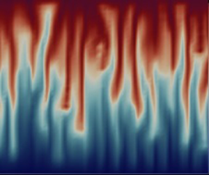
It is noted that the corresponding temperature profiles across the porous layer present little variation with time. However, the nanoparticle concentration may exhibit a fingering pattern, as demonstrated in figure 7. At  $t^* = 3.6$, as shown in figure 7(a), the concentration profile of nanoparticles is almost the same as the distribution at the initial state. The nanoparticles are more concentrated in the upper half of the porous layer due to the stronger thermophoretic effect (i.e. $N_E>0$). Once the flow velocity grows and exceeds a certain critical value, for example, as shown in figure 7(b) at $t^*= 4.0$, where the vertical flow velocity is greater than 0.2, the downward long narrow cells are triggered, which is similar to the salt fingers observed in double-diffusive convection (Huppert & Turner Reference Huppert and Turner1981). The fingering pattern develops further and is more apparent, as illustrated in figure 7(c) at $t^*= 4.4$. Obviously, the fingering pattern of nanoparticle concentration is induced by the growth of the narrow convection cells and the unstable density gradient. Note that the thermophoretic effect would develop an unstable vertical density gradient as the system is heated from below, while the effect of gravity settling would make an opposing contribution to reduce the upwards density gradient. Since the upper fluid layer is heavier due to the higher nanoparticle volume fraction, the presence of narrow convection cells acts to release the gravitational potential energy in the heavier nanofluid at the top. Such a fingering pattern also may provide more passages with higher thermal conductivity for heat conduction and thus enhance the heat transfer efficiency across the porous layer.

Figure 7. Temporal evolution of nanofluid concentration for the case of  $d_p=20$ nm at $Rn = 25$ and $Ra_D=7.7$: (a) $t^*=3.6$, (b) $t^*=4.0$ and (c) $t^*=4.4$.
5.2. Results of nanofluid with moderate-diameter nanoparticles
In this section, we consider the condition of a nanofluid composed of moderate-diameter nanoparticles to further examine the influence of the gravity settling effect. The typical case of  $d_p=40$ m was employed in the analysis, and according to (2.3a) and (3.8h), the parameter $N_g$ would be enlarged 8 times if the mean diameter of nanoparticles is doubled. Hence, the parameter $N_g$ increases to 11.12 and the other related dimensionless parameters are as follows: $Le=3.81 \times 10^5, \chi _A=2.50$ and $\chi _B=40916$. The variation of the neutral curves with $Rn$ is illustrated in figure 8. It is found that the neutral curves also descend and flatten gradually with increasing $Rn$. That is, the addition of nanoparticles with moderate diameter to the base fluid still presents a destabilizing effect on the system and a tiny concentration of nanoparticles is sufficient to produce a significant destabilizing effect. As $Rn$ exceeds $10^{-4}$, the minimum on the neutral curve approaches a constant but the corresponding critical wavenumber may vary with increasing $Rn$.
$Rn$.

Figure 8. Variation of neutral curves with  $Rn$ for the case of $d_p=40$ nm.
The corresponding variations of  $Ra_{D,c}$ and $k_c$ with $Rn$ are illustrated in figure 9(a,b), respectively. The results of the case in the absence of the gravity settling effect (i.e. $N_g = 0$) are also displayed for comparison. Obviously, the neglect of the gravity settling effect would cause unrealistic instability behaviours like the results observed in the case $d_p= 20$ nm as shown in figure 3. Once the effect of gravity settling was taken into consideration, the value of $Ra_{D,c}$ decreases first and then gradually approaches a constant 27.76. The variation characteristic is similar to the case $d_p= 20$ nm. However, for the critical wavenumber $k_c$, the variation is quite different from the case $d_p= 20$ nm. Instead of decreasing to nearly zero as observed in figure 3(b), it presents a slight reduction first and then rises with $Rn$ after $Rn>1$. The variation of $k_c$ in the high $Rn$ region is less important because the neutral curve would be a near horizontal line as $Rn$ is large enough, which indicates the instability for a wide range of wavenumber k would be very close at the onset of instability. The flow patterns for three typical $Rn$ values: 2.5, 25 and 250 are shown in figure 10(a–c), respectively. At lower nanoparticle concentration with $Rn = 2.5$, the convention cells almost occupy the whole thickness of the porous layer. As $Rn$ increases to 25, the wavenumber increases and the flow velocity rises, as indicated by the denser streamlines with a higher gradient of the streamfunction. The convection tends to concentrate in the middle region of the porous layer and the more vigorous flow may induce the weak small cells close to the upper and lower boundaries, as in the pattern at $Rn = 250$.

Figure 9. Variations of (a) the critical Rayleigh–Darcy number  $Ra_{D,c}$ and (b) the critical wavenumber $k_c$ with $Rn$ for the case of $d_p=40$ nm.

Figure 10. The flow patterns of onset convection cells for  $d_p=40$ nm: (a) $Rn = 2.5$ and $k_c=3.63$, (b) $Rn = 25$ and $k_c=5.82$ and (c) $Rn = 250$ and $k_c=7.02$.
The spectrum of growth rate for the state with  $Ra_D$ over the critical value is more attractive in practical conditions. Figure 11 shows the spectra of growth rate for three typical cases with higher $Ra_D$ than $Ra_{D,c}$ at $Rn= 25$. It is found that the spectrum of the growth rate rises with increasing $Ra_D$ and, for an assigned $Ra_D$, the growth rate exhibits an increase with wavenumber $k$, reaches a maximum and then decreases gradually. The unstable modes in the low- and high-wavenumber regions are obviously inhibited by the magnified gravity settling effect. On the other hand, the unstable modes with moderate wavenumbers are conspicuous and dominate the onset of instability. For example, as shown for the case $Ra_D= 28.2$, the most unstable modes occur approximately within the range $k = 4.7 \sim 5.0$. This result is quite different from the case of small nanoparticle diameter where the unstable modes with high wavenumbers determine the instability characteristics.

Figure 11. The spectra of growth rate  $s_r$ at $Rn = 25$ for three typical cases with $Ra_D>Ra_{D,c}$ ( $d_p=40$ nm).
The results of the numerical simulation for the flow patterns are illustrated in figure 12 with  $Rn = 25$ and $Ra_D= 28$. The other parameters used in the simulation are listed in table 2. The convection cells grow gradually with time, as shown in figure 12(a) for $t^*=1.0$. The flow pattern eventually approaches a steady form but the magnitude and gradient of the streamfunction continue to rise with time, as shown in figures 12(b) and 12(c) for $t^*= 3$ and 5, respectively, which indicates that the flow velocity increases continuously. In particular, we can estimate the wavenumber as approximately 4.4 within the two-dimensional domain with $a_r = 6$, which is in excellent agreement with the most unstable mode with $k_{max}=4.5$ as predicted in figure 11. Because the simulation was performed within a confined domain and we have taken the nonlinear coupling effects into consideration, this result reveals that the present model for direct numerical simulation can explore the instability behaviours precisely. After $t^*> 5$, the dimensionless flow velocity would be greater than 0.1, which is sufficient to induce the variations of nanoparticle concentration and temperature across the porous layer.

Figure 12. The evolution of the streamfunction at  $Rn = 25$ and $Ra_D=28$ for the case of $d_p=40$ nm: (a) $t^*= 1$, (b) $t^*= 3$ and (c) $t^*= 5$.
The evolution of nanoparticle concentration is demonstrated in figure 13. As  $t^*<5$, the flow velocity is too weak to induce variations in nanoparticle concentration and temperature. Hence, both the nanoparticle concentration and temperature profiles remain the same as those in the basic state. Once the convection cells develop to a certain extent after $t^*> 5$, the growing convective motion causes the concentration profile to transform into a wavy distribution, as shown in figures 13(b) and 13(c). The corresponding temperature profiles are displayed in figure 14. It is obvious that the temperature profile would be affected by the convection later than the concentration profile and then also begin to vary into a wavy form. The major reason is due to the high Lewis number of the nanofluid and the thermal diffusivity being generally much higher than the diffusivity of the nanoparticles. It is noted that, once the dimensionless flow velocity exceeds 1.0, the gradients of nanoparticle concentration and temperature will rise rapidly. Under such a condition, the local thermal equilibrium between the matrix of the porous medium and the nanofluid could be violated and then cause the deviation of the simulation result from the practical condition. In addition, according to the CFL convergence condition, the steeper gradient of nanoparticle concentration should accompany a smaller time step in the solution process to avoid the occurrence of divergence. This would consume much time and raise the cost of the simulation greatly. Therefore, it is crucial to perform the numerical simulation within an appropriate range of $t^*$ which is sufficient to obtain correct results for the nonlinear instability behaviours.

Figure 13. Temporal evolution of nanofluid concentration for the case of  $d_p=40$ nm at $Rn = 25$ and $Ra_D= 28$: (a) $t^*= 5$, (b) $t^*= 5.4$ and (c) $t^*= 5.8$.

Figure 14. Temporal evolution of temperature for the case of  $d_p=40$ nm at $Rn = 25$ and $Ra_D= 28$: (a) $t^*= 5$, (b) $t^*= 5.4$ and (c) $t^*= 5.8$.
Note that the fingering pattern of nanoparticle concentration was not observed at the condition of  $Rn = 25$. However, once the parameter $Rn$ increases further, which indicates a higher nanoparticle concentration and thermophoretic diffusion effect, the dimensional density gradient across the porous layer would be raised and the onset of fingering convection can still be triggered. As shown in figure 15, in which $Rn$ increases to 250, the onset of nanoparticle convection occurs at approximately $t^*=6$, as illustrated in figure 15(a), due to the higher thermophoretic effect indicated by (2.3c), and then the fingering convection of nanofluid concentration emerges and grows gradually with time. It is found that, as shown in figure 16, the spectrum of the growth rate from the linear stability analysis for $Rn = 250$ presents a similar pattern to figure 5. That is, the unstable modes in the high-wavenumber region present comparable growth rates. Hence, the onset of instability would be dominated by the unstable modes with high wavenumbers again and the resultant long narrow convection cells cause the occurrence of a fingering pattern once the convection magnitude is strong enough.

Figure 15. Temporal evolution of nanofluid concentration for the case of  $d_p=40$ nm at $Rn = 250$ and $Ra_D= 28$: (a) $t^*= 6$, (b) $t^*= 6.5$ and (c) $t^*= 7$.

Figure 16. The spectra of growth rate  $s_r$ at $Rn = 250$ for three typical cases with $Ra_D>Ra_{D,c}$ ( $d_p=40$ nm).
5.3. Results of nanofluid with large-diameter nanoparticles
The effect of gravity settling exerts a significant stabilizing effect on the system stability as the mean diameter of the nanoparticles increases. Since a nanoparticle diameter within the range of  $20 \sim 60$ nm is commonly used in nanofluids, in this section, we further consider the typical case of a nanofluid with a lager nanoparticle diameter of 60 nm. The effect of gravity settling would be enlarged 27 times relative to the case of $d_p= 20$ nm. Hence, the instability characteristics are expected to be different from those of a nanofluid with a smaller nanoparticle diameter. The corresponding dimensionless parameters are as follows: $Le=5.72\times 10^5$, $N_g=37.54$, $\chi _A=1.66$ and $\chi _B=4.09\times 10^4$. The variation of the neutral curves with $Rn$ is shown in figure 17(a). As $Rn$ is less than 0.01, the nanoparticle concentration is too low to have any apparent influence on the flow instability. The critical value of $Ra_D$ is still quite close to the theoretical value 4 ${\rm \pi} ^2$ of the case for the porous layer saturated with pure viscous fluid and only the stationary mode can be observed on the neutral curve. Once the nanoparticle concentration increases with $Rn$ over 0.01, however, in contrast to the small- and moderate-diameter nanoparticles, the nanofluid with large-diameter nanoparticles exhibits enhanced flow stability. The neutral curve never dips lower but rises gradually with increasing $Rn$. In particular, the oscillatory mode emerges on the neutral curve in the range of wavenumber from 1.5 to 6.4, as shown in figure 17(b), and the oscillatory frequency grows gradually with increasing $Rn$. This result reveals the significance of the gravity settling effect, which is a strong stabilizing factor and may induce the onset of the oscillatory mode.

Figure 17. Variations of (a) neutral curves with  $Rn$, and (b) the corresponding oscillatory frequency for the case of $d_p=60$ nm.
To demonstrate the linear stability characteristics clearly, the variations of  $Ra_{D,c}$, $k_c$ and the magnitude of the critical oscillatory frequency $|s_{i,c}|$ with $Rn$ are respectively illustrated in figure 18(a–c). One can see that $Ra_{D,c}$ is equal to 39.47 and almost invariable until $Rn$ is greater than 0.1, then $Ra_{D,c}$ rises and the corresponding value of $N_A$ approaches $N_g$ eventually. This result verifies the instability mechanism again that the stability of nanofluid flow is dominated by the relative strength of thermophoresis to gravity settling. Once the effect of thermophoresis prevails over the effect of gravity settling, the system would become unstable. Therefore, a larger nanoparticle diameter would produce a stronger gravity settling effect that makes the critical value of $Ra_D$ rise. In other words, the system tends to be more stable. In particular, it is noted that the equivalent parameter $N_A$ approaches $N_g$ in the negative direction of $N_g$ with increasing $Rn$ (i.e. $N_E<0$), which is different from the two cases of small- and moderate-nanoparticle diameters. That is, the upward gradient of nanoparticle volume fraction is always negative at the critical state with a stably stratified distribution in the basic state. Under such a condition, the contribution of nanoparticle concentration to nanofluid density is opposite to the contribution of thermal instability, and the interaction between the destabilizing effect of thermophoresis and the stabilizing effect of gravity leads to the result that the oscillatory mode prevails over the stationary mode and dominates the onset of instability. Note that, when the thermophoretic effect is strong enough to produce an unstable profile of nanofluid concentration, the oscillatory mode vanishes and the stationary mode dominates again. If the effect of gravity settling is ignored, one would obtain unrealistic results of unconditional instability again, as in the red curves shown in figure 18 with $N_g= 0$. The variation of $k_c$ is limited and it first decreases slightly from 3.14 to 3.06, and then becomes constant at 3.14 again. The variation of $|s_{i,c}|$ is remarkable and it begins to rise as $Rn> 10^{-3}$, and then approaches a constant of 14.1.

Figure 18. Variations of the critical values (a)  $Ra_{D,c}$, (b) $k_c$ and (c) $|s_{i,c}|$ with $Rn$ for the case of $d_p=60$ nm.
Three typical flow patterns of the oscillatory mode are shown in figure 19. At  $Rn = 2.5$, the oscillatory convection cells are inclined and occupy the whole thickness of the porous layer. As $Rn$ increases to 25 and 250, as shown in figures 19(b) and 19(c), respectively, the inclined convection cells gradually turn into square cells with higher oscillatory frequency. The gradient of the streamfunction presents infinitesimal variation in these flow patterns, which implies the convection magnitudes at the onset of instability are almost equivalent in these cases. The variations of growth rate $s_r$ and the corresponding magnitude of the oscillatory frequency $|s_i|$ for several typical cases with $Ra_D> Ra_{D,c}$ at $Rn = 25$ are respectively shown in figures 20(a) and 20(b). It is found that the unstable modes appear as $Ra_D > 61.2$, and the spectrum extends and rises gradually with $Ra_D$. However, the corresponding oscillatory frequency $|s_i|$ decreases with increasing $Ra_D$, as shown in figure 20(b). The most unstable mode with the maximum growth rate moves gradually to the right from $k_{max} = 3.14$ at $Ra_D = 61.3$ to $k_{max} = 3.6$ at $Ra_D = 62$. Note that, once $Ra_D$ is close to 62.33 (i.e. $N_A> N_g$), the stationary mode would emerge on the spectrum and gives the maximum growth rate, as shown in figure 20(a). The profile of nanofluid concentration would become unstably stratified at the basic state. As a result, the most unstable mode would be replaced by the stationary mode with $|s_i|=0$. After $Ra_D>62.33$, the stationary mode on the spectrum extends gradually, while the oscillatory mode recedes and then vanishes eventually. The spectra of the cases with $Ra_D>62.33$ in figure 20(a) are all stationary modes and the variation is similar to the result displayed in figure 11.

Figure 19. The flow patterns of onset convection cells for  $d_p=60$ nm: (a) $Rn = 2.5$, $k_c=3.07$, $Ra_{D,c} =52.32$ and $|s_{i,c}|= 7.7$, (b) $Rn = 25$, $k_c= 3.14$, $Ra_{D,c} =61.21$ and $|s_{i,c}|= 13.64$, (c) $Rn = 250$, $k_c=3.14$, $Ra_{D,c} =62.33$ and $|s_{i,c}| = 14.09$.

Figure 20. (a) The spectra of growth rate  $s_r$ at $Rn = 25$ for several typical cases with $Ra_D>Ra_{D,c}$ ( $d_p=60$ nm), and (b) the corresponding magnitudes of oscillatory frequency $|s_i|$. (The solid and dashed lines indicate the stationary (ST) and the oscillatory (OS) modes, respectively.)
The onset of the oscillatory mode was verified by numerical simulation and the results are demonstrated in figure 21 for the evolution of flow patterns with time at  $Rn = 25$ and $Ra_D= 62$. The other parameters are listed in table 2. Square convection cells are observed and, in particular, the convection cells become travelling waves and oscillate in the horizontal direction. The convection magnitude also presents oscillation but generally grows with time. The wavenumber oscillates in the range from 3.14 to 3.66, which is consistent with the result of linear stability analysis that the most unstable mode is determined by the oscillatory modes near $k_{max} = 3.6$. The oscillatory frequency is not a constant but varies with time. The difference between the results of linear stability analysis and direct numerical simulation is primary due to the confined domain in numerical simulation, while the horizontal porous layer is assumed to extend infinitely in horizontal direction. However, the results of numerical simulation are still in excellent agreement with the instability behaviours predicted by the linear stability analysis. The corresponding profiles of nanofluid concentration are shown in figure 22. It is noted that, at $Ra_D = 62$, the parameter $N_E$ is negative, which results in a stably stratified nanofluid layer at the basic state, as indicated in figure 22(a). Once the convection of oscillatory cells is strong enough, we can observe the wavy profile of nanofluid concentration, as shown in figure 22(b). The wavy pattern grows gradually and oscillates as travelling waves in the horizontal direction, as illustrated in figure 22(c). A supplementary movie, available at https://doi.org/10.1017/jfm.2024.124, shows the temporal behaviour of the travelling wavy patterns.

Figure 21. The evolution of oscillatory flow patterns at  $Rn = 25$ and $Ra_D= 62$ for the case of $d_p=60$ nm: (a) $t^*=6.01$, (b) $t^*=6.26$ and (c) $t^*=6.74$ (see supplementary movie).

Figure 22. Temporal evolution of nanofluid concentration for the case of  $d_p=60$ nm at $Rn = 25$ and $Ra_D= 62$: (a) $t^*= 6.01$, (b) $t^*= 6.26$ and (c) $t^*= 6.74$ (see supplementary movie).
The fingering pattern of nanofluid concentration still can be observed when  $Rn$ increases with $N_E>0$. For example, at $Rn = 250$ with $Ra_D = 63.5$, the spectrum of the growth rate presents the same form as in the case $Ra_D = 28$ or 28.2 in figure 16. Moreover, the growth rate is much higher and would exceed 100 in the high-wavenumber region and the density difference across the porous layer is significant in an unstably stratified distribution. Therefore, the onset of a fingering pattern of nanofluid concentration would be triggered quickly by the unstable modes with high wavenumbers, as revealed in figure 15.
6. Conclusions
The thermal instability in a horizontal porous layer saturated with a nanofluid was investigated in this study. The Darcy model was used for the high-porosity porous layer and the diffusion of nanoparticles was simulated by the revised Buongiorno model, in which the effect of gravity settling was taken into consideration. By linear stability analysis, the stability characteristics were found to depend heavily on the size of the nanoparticles. For a nanofluid with a smaller mean diameter of nanoparticles, the effect of thermophoresis is more pronounced than the effect of gravity settling, which results in a highly unstable density profile across the porous layer. As a result, the system was destabilized significantly. In addition, once  $Ra_D$ exceeds the critical value, the spectrum of growth rate behaves as a flat line in the high-wavenumber region to govern the onset of instability. The convection would present in the form of small narrow convection cells, which has been verified by direct numerical simulation. In particular, the narrow convection cells may trigger the occurrence of a fingering pattern of nanofluid concentration, which could be a possible mechanism to enhance the heat transfer efficiency across the layer. For the case of a nanofluid with a larger size of the nanoparticle diameter, the gravity settling effect would be enlarged to balance the thermophoretic effect. Hence, the flow would be stabilized by employing the nanofluid and the onset of instability would be dominated by the oscillatory mode if the gravity settling effect is large enough to produce a stably stratified nanofluid concentration at the basic state. However, if the nanofluid concentration is lower, the convection cells would not induce the appearance of a fingering pattern of the nanofluid concentration but instead a pattern in the form of travelling waves. If the nanofluid concentration is large enough, the fingering pattern still can be observed once the thermophoretic effect prevails over the gravity settling effect to produce an initially unstably stratified nanofluid concentration profile. Notice that the heat transfer efficiency, or Nusselt number, is not discussed in this work. The main reason for this relates to the assumptions made in the present model. Since this study aims to explore the effect of the gravity settling of nanoparticles on the onset of Darcy-type Rayleigh–Bénard convection, it is appropriate to assume the conditions of local thermal equilibrium, constant thermophysical properties and negligible mechanical dispersion effects. However, the interstitial heat transfer between the fluid and solid matrix may become significant when the flow velocity is high (Zhang et al. Reference Zhang, Li and Nakayama2015) and the effect of mechanical dispersion could be more dominant than molecular diffusion. The present results reveal that, unlike pure fluid systems, convection in nanofluid systems beyond the critical condition is usually violent, even at low Rayleigh number. As shown by the present linear stability analysis and numerical simulation, the induced velocity grows quickly at a finite time after the onset of convection, which may cause the assumptions break down already. Thus, the present numerical simulations are valid only in a short period of time after the onset of instability. Nevertheless, the numerical simulations in this work confirm the results of linear stability analysis. It also provides a preliminarily understanding of the flow characteristics after the onset of convection. The other reason is due to the difficulty arising from the numerical method itself. Even though we ignore the failure of the assumptions, it is still difficult to proceed with calculation once the steep concentration gradients appear in the flow field after a longer time. Briefly, the diffusion of nanoparticles caused by Brownian motion is much slower than thermal diffusion, which causes an extremely high Lewis number for the nanofluid in comparison with general solute fluids. This inevitably leads to great difficulties in numerical calculations. In fact, the migration of nanoparticles tends to induce high concentration gradients within the flow structure because the time scale of nanoparticle diffusion is much longer than the other characteristic times. This phenomenon implies that a finer mesh structure and a smaller time step are required in the simulations. That is, the simulation of vigorous convection far beyond the critical condition would be quite costly but could be studied further in the future.
The present results reveal that the flow tends to be destabilized by using smaller nanoparticles in the composition of the nanofluid. The work also promotes the occurrence of fingering convection of nanoparticles in the porous layer. On the contrary, a larger nanoparticle size would stabilize the flow and a higher temperature difference is required to trigger the onset of convection. A three-dimensional numerical simulation in the future would benefit our understanding of the structure of thefingering pattern of the nanofluid concentration and the mechanisms that induce this flow instability behaviour. An experimental study is also very interesting and important to observe the possible occurrence of fingering convection in a nanofluid-saturated porous layer and confirm the present numerical predictions.
Supplementary movies
Supplementary movies are available at https://doi.org/10.1017/jfm.2024.124.
Funding
The support for this work from the National Science and Technology Council of Taiwan through the grant number NSTC 112-2221-E-197-019 is gratefully acknowledged.
Declaration of interests
The authors report no conflict of interest.


