


1. Introduction
Glacier changes are widely recognised as key indicators of climate change (e.g. Vaughan and others, Reference Vaughan, Stocker, Qin, Plattner, Tignor, Allen, Boschung, Nauels, Xia, Bex and Midgley2013), meaning that they respond very sensitively to small changes in climatic conditions. In particular, the dramatic retreat of glaciers in nearly all regions of the world over the past century has demonstrated the impacts of atmospheric warming for a large public (Zemp and others, Reference Zemp2015; Rastner and others, Reference Rastner, Joerg, Huss and Zemp2016). Mass-balance measurements are more challenging to perform compared to length-change measurements, but easier to interpret as they represent a direct and undelayed response to the atmospheric forcing. Thereby, long-term time series of glacier mass balance serve several purposes, for example: (1) detection of climate trends, (2) spatio-temporal extrapolation of their contribution to sea-level (Marzeion and others, Reference Marzeion, Jarosch and Hofer2012; Gardner and others, Reference Gardner2013; Giesen and Oerlemans, Reference Giesen and Oerlemans2013; Radić and others, Reference Radić2014; Huss and Hock, Reference Huss and Hock2015), (3) determination of their contribution to run-off and regional hydrology (Casassa and others, Reference Casassa, López, Pouyaud and Escobar2009; Kaser and others, Reference Kaser, Grosshauser and Marzeion2010; Huss, Reference Huss2011; Carturan and others, Reference Carturan2019), (4) calibration and validation of numerical models (e.g. Huss and Farinotti, Reference Huss and Farinotti2012) and (5) calculation of crustal uplift (Barletta and others, Reference Barletta2006; Dietrich and others, Reference Dietrich2010), among others.
For all of the above applications, the most severe issue is the disappearance of a reference glacier (Cogley and others, Reference Cogley2011) with a long time series, when climatic conditions are no longer suitable for its survival. Unfortunately, this is not only a problem in the Alps (e.g. Carturan and others, Reference Carturan2013a; Thibert and others, Reference Thibert, Eckert and Vincent2013), but is occurring in several other regions of the world with strong glacier decline (e.g. Ramirez and others, Reference Ramirez2001; Mölg and others, Reference Mölg2017; Prinz and others, Reference Prinz, Heller, Ladner, Nicholson and Kaser2018). The disappearance of mass-balance glaciers with a long-term record has already been recognised in earlier studies (e.g. Haeberli and others, Reference Haeberli, Hoelzle, Paul and Zemp2007, Reference Haeberli, Huggel, Paul, Zemp, Shroder, James, Harden and Clague2013) as a serious issue for the continuation of long-term glacier monitoring strategies. In regions with sparse measurements this loss is particular unfortunate, as it considerably increases the uncertainty of the related regional-scale estimates of annual glacier mass loss (e.g. Zemp and others, Reference Zemp2019).
As the value of a mass-balance time series increases with its length, the loss of such time series is regrettable. It increases the uncertainty of any regional scale extrapolation up to a point where it is no longer possible (e.g. in regions with only a few measured glaciers). At best, a nearby glacier is found in time as a replacement to have parallel measurements over a sufficient period (Carturan, Reference Carturan2016; Galos and others, Reference Galos2017). However, as there is a high glacier-to-glacier variability in mass-balance time series (e.g. Kuhn, Reference Kuhn1985), the new glacier might have different characteristics, altering the regionally averaged mass-balance time series. Apart from missing mass-balance data, the loss of glaciers in general might have other severe impacts on human well-being, for example in regions depending on glacier meltwater, be it for agriculture, run-off regulation or hydropower production (e.g. Vergara and others, Reference Vergara2007; Sorg and others, Reference Sorg, Bolch, Stoffel, Solomina and Beniston2012; Lutz and others, Reference Lutz, Immerzeel, Kraaijenbrink, Shrestha and Bierkens2016), for tourism or as a source of natural hazards once bare rock and unconsolidated debris are exposed (e.g. Ritter and others, Reference Ritter, Fiebig and Muhar2012; Huggel and others, Reference Huggel, Carey, Clague and Kääb2015; Mark and Fernández, Reference Mark and Fernández2017; Zanoner and others, Reference Zanoner2017). Unfortunately, we have also limited countable evidence on the glaciers that have disappeared since a certain point in time, which resulted in an underestimation of their contribution to sea-level rise (Parkes and Marzeion, Reference Parkes and Marzeion2018). Thereby, defining when a glacier has actually disappeared is a challenge (Leigh and others, Reference Leigh2019).
Long before a glacier disappears due to climate change, reinforcement feedbacks might start to interfere and create a more negative mass balance than expected from climatic change alone, i.e. causing a disequilibrium response (Pelto, Reference Pelto2010). In particular, down-wasting with disintegration into several smaller glacier parts has a very negative impact on mass balance as glacier tongues are separated from the accumulation area, and thermal radiation from rock outcrops, combined with decreased cooling effects over smaller glaciers, can enhance melt considerably (e.g. Greuell and Böhm, Reference Greuell and Böhm1998; Greuell and others, Reference Greuell, Knap and Smeets1997; Carturan and others, Reference Carturan, Cazorzi, De Blasi and Dalla Fontana2015). A key question is thus if the disequilibrium response of a glacier can be identified in its mass-balance time series, so that the glacier can be removed from regionally averaged mass-balance values in retrospect. Despite intense use of mass-balance time series for numerous applications (see above), this aspect has so far not been analysed and considered. Accordingly, calculations using these time series as an input (e.g. for model calibration) might be biased and generate wrong results. A first aim of this study is thus to identify related shifts in the mass-balance regime of glaciers in the Alps with long-term observations.
A second aim of this study is to characterise the larger sample of glaciers with mass-balance measurements (I) topographically (e.g. hypsometry, breaks in slope, aspect and elevation range) and (II) by a set of further criteria related to their overall health and vulnerability. Health criteria include (a) a continued negative mass balance despite strong shrinkage (requires area change analyses), (b) a potential disequilibrium response with mass loss in the accumulation area (requires elevation change analyses), (c) the size of the accumulation area at the end of the ablation season (requires analysis of satellite image time series) and (d) flow velocities close to zero (Stocker-Waldhuber and others, Reference Stocker-Waldhuber, Fischer, Helfricht and Kuhn2019) combined with collapse of subglacial cavities (requires space-borne and field observations). By investigating these factors, this analysis should reveal the vulnerability of the currently measured glaciers in the Alps in view of the anticipated further temperature increase (Kotlarski and others, Reference Kotlarski2014), and provide useful criteria for replacing disappearing glaciers with long-term mass-balance series in good time.
In this study, we have investigated topic (I) and points (a) to (c) of topic (II) for 46 glaciers with mass-balance measurements in the Alps. We have used time series of satellite imagery to determine area changes and snowline variability, as well as digital elevation models (DEMs) from two points in time to determine the elevation change patterns among the glaciers. For a smaller sample of nine glaciers with long-term mass-balance records, we have analysed in detail each time series in comparison with the others (to analyse regional variability and find the regime shifts) along with the analysis of their vulnerability to determine possible reasons for their disequilibrium response. Ultimately, we applied the vulnerability index to all measured glaciers in the Alps indicating which of them might be impacted next by non-climatic effects on their mass balance.
2. Study region
The European Alps (called ‘Alps’ hereafter) are an arc-shaped mountain range that is ~1500 km long, stretches from 2° to 18° E and 43° to 49° N, and is subdivided by the administrative boundaries of nine different countries (Austria, Croatia, France, Germany, Italy, Liechtenstein, Monaco, Slovenia and Switzerland). Its elevation averages ~2500 m a.s.l., peaking at Monte Bianco/Mont Blanc with 4810 m a.s.l. (Fig. 1). The Alps are affected by air masses of very different origins: mild and moist maritime air from the west, cool or cold polar air from north, dry and warm (in summer) or cold (in winter) continental air from east and warm African or Mediterranean air (sometimes very wet) from south. As the Alps constitute an important obstacle to the transit of moist air masses, they give rise to high horizontal and vertical gradients in precipitation. Annual precipitation amounts range from ~400–500 mm at valley floors in the drier inner regions to 3000–3500 mm in the wettest areas (e.g. Jungfrau and Julian Prealps) (Isotta and others, Reference Isotta2014). Accordingly, there is a strong gradient in glacier mean elevation from the wetter outer regions at ~2600 m a.s.l. to the drier interior at ~3200 m a.s.l. (Paul and others, Reference Paul, Frey and Le Bris2011). Climatic conditions range from slightly maritime to slightly continental and many glaciers are not strictly temperate but rather polythermal, with probably cold surface layers in the ablation area (Haeberli and Hoelzle, Reference Haeberli and Hoelzle1995), or with cold firn and ice at high altitudes (Suter and others, Reference Suter, Laternser, Haeberli, Frauenfelder and Hoelzle2001). Whereas there is no significant trend in precipitation amounts over the past 150 years, temperatures increased ~1°C between 1850 and 1980, and have increased an additional degree since 1980 (Auer and others, Reference Auer2007).

Fig. 1. Geographic location of the mass-balance glaciers in the European Alps that have been analysed in this study.
In 2015/16, there were 4394 glaciers larger 0.01 km2 in the Alps with different types (valley, mountain, hanging, cirque and plateau), covering a total area of 1806 km2 (Paul and others, Reference Zemp2020). The region is dominated by small glaciers (92% are <1 km2 covering 28% of the area). However, the 21 largest glaciers (>10 km2) contribute only 0.5% to the total number of glaciers but cover about the same area (26% of the total). Regular measurements of changes in glacier length (or terminus position) have been performed in the Alps since 1894 (Forel, Reference Forel1895), starting with 85 glaciers and now being at 270. They provide the backbone of our knowledge about glacier fluctuations in the Alps (e.g. Holzhauser and others, Reference Holzhauser, Magny and Zumbühl2005; Zemp and others, Reference Zemp2015) and have been widely used for numerical modelling of past climate variability (e.g. Oerlemans, Reference Oerlemans2005; Goosse and others, Reference Goosse2018), as well as numerous other applications in hydrology and climate change research.
The first mass-balance measurements in the Alps were carried out on Rhône Glacier in the period from 1884 to 1909, using the glaciological method (Huss and others, Reference Huss, Dhulst and Bauder2015). This method is based on the spatial extrapolation of thickness changes measured at least annually (at the end of the hydrological year) at stakes and snow pits using the glacier hypsometry. These are converted to water equivalent (w.e.) by multiplication with the density of ice and field-based measurements of snow and firn densities (Kaser and others, Reference Kaser, Fountain and Jansson2003). The longest continuous series of mass-balance measurements for an entire glacier date back to 1948 (Sarennes). The sample was extended in the following decades and is now at 46 glaciers per year.
Continuous series longer than 30 years currently exist for 40 glaciers worldwide and 11 in the Alps. Time series of mass-balance values for glaciers in Switzerland show a large variability of the cumulative mass balance from glacier to glacier, but also some common trends: clear mass gains before the 1920s and 1980s, and fast mass loss in the 1940s and since about 1985 (Huss and others, Reference Huss, Dhulst and Bauder2015). It is assumed that the latter is related to a switch in the global climate regime (Reid and others, Reference Reid2016). The current mean specific mass loss of ~1 m w.e. a−1 multiplied with a glacier area of ~2000 km2 (Paul and others, Reference Paul, Frey and Le Bris2011) gives an average mass loss of 2 Gt a−1 for the Alps. Assuming a residual ice volume of ~70–100 km3 in the Alps in 2018 (Haeberli and others, Reference Haeberli, Oerlemans and Zemp2019), complete glacier loss might be expected in 50 years at current rates of depletion.
3. Data sets
To ease calculations and comparisons across glaciers, we distinguish the three samples marked in Figure 1, namely Sample A: all glaciers, Sample B: 46 glaciers with mass-balance measurements between 2004 and 2013 and Sample C: nine glaciers with continuous long-term measurements since 1967. Sample B is included in Sample A and Sample C is included in both samples A and B.
3.1 Glacier outlines (O1 and O2)
Glacier outlines from 2003 (Paul and others, Reference Paul, Frey and Le Bris2011) and 2006 (Salvatore and others, Reference Salvatore2015) have been used as starting conditions for all glaciers. This dataset (O1 in the following) represents Sample A. To determine area changes for Sample B, a second dataset of glacier outlines (O2) was created using Landsat 7 and 8 scenes of the years 2013 and 2015. These new outlines were obtained by automatic classification of clean ice using the band ratio method and manual post-processing (e.g. to correct unclassified debris-covered glaciers) following Paul and others (Reference Paul2009).
3.2 DEMs (D1, D2 and D3)
Three different DEMs have been used for calculating topographic parameters and elevation changes. Topographic parameters for samples A and B were extracted from the 30 m ASTER GDEM2 (D1) that is a merged product using ASTER scenes acquired between 2000 and 2012. Although this DEM has local quality issues, it has no data voids and was available also for the very small glaciers in the sample. Glacier elevation changes were calculated by differencing the 1 arcsec (~30 m) SRTM DEM acquired in 2000 (D2) from the 1 arcsec TanDEM-X DEM acquired about 2012–14 (D3) for the entire Alps. We have not corrected data voids or issues related to radar penetration as we were mostly interested in the pattern of the changes rather than correct absolute values. However, to be aware of the possible issues related to these DEMs, we have compared the elevation changes from SRTM and TanDEM-X with changes derived from two high-accuracy LiDAR DEMs with a cell size of 0.5 m obtained by surveys in 2003 and 2013 and commissioned by the University of Padova. This comparison was restricted to La Mare and Careser glaciers in the Ortles-Cevedale Group in Italy.
3.3 Ice thickness distribution
We used the distributed ice thickness dataset by Huss and Farinotti (Reference Huss and Farinotti2012) for calculation of an ice thickness index (ITI). The dataset provides physically-based ice thickness estimates for individual glaciers and is based on glacier outlines from 2003 (O1) to spatially constrain the modelling and the SRTM DEM (D2) for topographic information (e.g. surface slope and hypsometry).
3.4 Mass-balance data
Mass-balance data are collected in the field and distributed by the World Glacier Monitoring Service (WGMS). Apart from mean annual values, we also extracted values of the accumulation area ratio (AAR) and equilibrium line altitude (ELA) for the 46 glaciers of Sample B (including the nine from Sample C). The period from 2004 to 2013 was selected on the basis of available data to characterise their recent status and variations. All glaciers of Sample B are used for correlation and vulnerability analyses, whereas the mass-balance time series of glaciers in Sample C are analysed in more detail. The analysed glaciers in Samples B and C are rather well distributed over the glacierised regions of the Alps (Fig. 1). Twelve of them are located in Austria, 14 in Italy, 14 in Switzerland and six in France (Table S1).
3.5 Satellite data
Apart from the selected satellite scenes used to create the recent glacier outlines (O2) for Sample B, we also used the time series of Landsat 5, 7 and 8 to derive snow cover maps over the 2004–2013 period for the 46 glaciers of Sample B, following Rastner and others (Reference Rastner2019). From the maps showing minimum snow extent within each year we calculated the snow cover fraction (SCF) and snowline altitude (SLA) based on the ASTER GDEM II for each glacier. As not all years had scenes close to the end of the ablation period, both SCF and SLA values are expected to be different from the AAR and ELA values measured at each glacier. This possible discrepancy is quantified and discussed in Section 6.3.
4. Methods
In Figure 2 we present a schematic overview of the datasets used and calculations performed based on the three samples displayed in Figure 1. The topographic comparison between samples A and B should reveal how similar or representative the glaciers with mass-balance measurements are compared to the entire sample of glaciers in topographic terms. For the 46 glaciers in Sample B we performed a detailed analysis of their morphometric characteristics as well as their area and elevation changes using the datasets described in Section 3. Afterwards, the observed variability in morphometric characteristics and geometric changes is reduced to four classes for selected criteria, indicating increasing vulnerability (see Section 4.2). Moreover, together with recent mass-balance variability in the decade from 2004 to 2013, morphometric characteristics are compared in a correlation analysis to reveal major dependencies among them (see Supplementary material). Finally, we perform a spatio-temporal analysis of the mass-balance variability of Sample C, and compare cumulative differences from the mean mass balance with an index that is derived as the sum of the individual vulnerabilities for all glaciers in Sample B (Section 4.2.1).

Fig. 2. Schematic overview of the datasets used and methodological flow chart. The abbreviations (D1, D2, D3, O1 and O2) are explained in the text; ‘mb’ is mass balance, ‘Sat’ is Satellite.
4.1 Topographic statistics (Sample A vs B)
For the comparison of samples A and B we calculated frequency distributions of several topographic parameters for both samples, using the outlines from 2003 and 2006 (O1) and the ASTER GDEMv2 (D1). The former provided glacier areas for deriving a size class distribution, and outlines combined with the DEM are used to derive histograms of elevation range, mean elevation, mean slope and aspect sector, using zone statistics.
4.2 Morphometric characteristics and changes (Sample B)
4.2.1 Vulnerability index
The vulnerability of each glacier of Sample B was calculated as an index that combines nine different vulnerability criteria (Table 1). The index, named glacier vulnerability index (GVI), expresses the possibility for a glacier to exist for a shorter or longer monitoring period in the future. It is conceived as a method to support evaluation of the suitability of different glaciers for future mass-balance monitoring programmes, rather than as a prognostic tool. Although the GVI includes criteria that account for favourable topographic conditions, its application is not recommended for glaciers that are too small (area <0.5 km2), because their mass balance tends to decouple from atmospheric forcing.
Table 1. Vulnerability criteria and ratings used for calculating the GVI for the 46 mass-balance glaciers of the European Alps. Outl. = Outline, Sat. = Satellite

a Elevation range is calculated excluding the 2nd and 98th percentiles in the hypsometric curve.
The nine vulnerability criteria reflect the dominant processes that govern glacier response and geometric adjustment, and can be derived from readily available input data. This makes the classification potentially applicable to other unmeasured glaciers (e.g. glaciers that might replace them). A rating from 1 to 4, expressing increased vulnerability, was assigned to each glacier based on the analysis of frequency distributions, indications from literature (e.g. Jiskoot and others, Reference Jiskoot, Curran, Tessler and Shenton2009 for the hypsometric index (HI)) and in the correlation among variables (see Tables 1, 2 and S2). The chosen thresholds are specific for the glacier geometries of the Alps (e.g. for elevation change or range) and the range of changes observed. They would thus have to be adjusted inother regions. The proposed class assignments might include a large range of possible absolute values or even neglect them when the focus is on the pattern of the change (e.g. gradients in different parts of a glacier). In the latter case, they are almost unaffected by small changes in absolute values (e.g. due to DEM uncertainties, glacier extent change or radar penetration). Total sums of the rating for all criteria constitute the GVI of each glacier. As a starting point, we used integer classes only and have given equal weight to all criteria, but lumped a few of likely local importance and auto-correlated (e.g. shadow, debris cover and avalanche contribution) into a single index. Tests have shown that the different weighting of the indices has small impacts on the GVI ranking of a glacier, but the general position remains similar. With the nine criteria and the four classes we use here, GVI values can range from 9 to 36. In the following subsections we describe each criterion together with its calculation and the four classes.
Table 2. Count of each vulnerability criterion and class for the 46 mass-balance glaciers of the European Alps

a Elevation range is calculated excluding the 2nd and 98th percentiles in the hypsometric curve.
4.2.2 Area change index (criterion 1)
Area changes result from the combination of elevation changes and ice thickness distribution. As such, they are indicative of past imbalance but also of possible future developments (Pelto, Reference Pelto2010). For example, a glacier that shows limited area changes only close to its terminus seems to be less vulnerable than a glacier that lost area along its entire perimeter and/or is disintegrating into several pieces (Paul and others, Reference Paul, Kääb, Maisch, Kellenberger and Haeberli2004). We have considered here area changes from 2003 to 2015, and separated them between the upper and lower parts of a glacier, according to the following area change index (ACI):

where AC u, AC l and AC t are percent area changes in the upper 55%, lower 45% and total (100%) of the glacier, respectively. The partition was done considering that on a global average the AAR related to a balanced mass budget is ~0.58 (Dyurgerov and others, Reference Dyurgerov, Meier and Bahr2009). Large ACI values (>0.3) mean large overall area loss and/or significant contribution from the upper part of the glacier to the total loss of area (class 4), whereas low ACI values (<0.05) indicate small total area loss and/or a small contribution from the upper glacier part, suggesting a lower vulnerability (class 1). Values in between have been assigned to classes 2 and 3 (cf. Table 1).
In Figure 3 the area changes for the nine mass-balance glaciers of Sample C are shown, clearly revealing the large variability in possible changes. They range from the disintegration of Careser and Sarennes (class 4) to comparably smaller changes limited to the ablation area of Kesselwand and Sonnblick (class 1).

Fig. 3. Area change of glaciers with continuous long-term measurements (Sample C) from 2003/06 to 2013/15.
4.2.3 Elevation change pattern (criterion 2)
Glaciers that show thinning up to their highest elevations on decadal timescales are likely to disappear (Pelto, Reference Pelto2010). In the southern Ötztal Alps, patterns of elevation change show a high degree of variability, even within this small region (Fig. 4). This includes the minor elevation loss of Kesselwand near the terminus (class 1), the more extended regions of loss in the ablation region at Hintereis and Vernagtferner (class 2), and surface lowering impacting the entire area at Hochjochferner (class 4).

Fig. 4. Elevation change calculated between the SRTM DEM and TanDEM-X DEM in the Ötztal region (Austrian Alps). Three mass-balance glaciers are highlighted with thicker outlines (H = Hintereis, K = Kesselwand, V = Vernagt), Hjf is Hochjoch Ferner.
We have analysed elevation changes between 2000 and 2013 in relation to the planimetric distance from the terminus, drawing manually a centre line for each glacier and then extracting the elevation change for each cell of the D3-D2 grid (Fig. 2), along the centre line. To compare glaciers of different lengths, we have normalised the distance from the terminus by dividing it by the total glacier length. The plots in Figure 5 show the four classes of elevation change patterns, which are defined by the magnitude of elevation changes in different parts of the glacier, their spatial variability and their elevation dependence (cf. Table 1): class 1 represents glaciers with low variability and little elevation change. This class includes only three glaciers, Adler and Timorion that have high mean elevations (3459 and 3306 m, respectively), and Kesselwand that has a large accumulation area above 3200 m (top-heavy).

Fig. 5. Elevation change averaged along longitudinal profiles of Sample B glaciers, clustered into four elevation change pattern classes.
Class 2 includes nine glaciers that show minor elevation changes in their upper half and large thinning in their lower half, with high elevation dependence. This behaviour is typical of glaciers in ‘active retreat’, which are shrinking almost exclusively at their lower margins but still preserve an accumulation area, i.e. with no elevation loss or even a small gain (e.g. Sonnblick and Vernagt).
Class 3 includes 20 glaciers showing higher imbalance, where thinning was larger and significant also in their upper half. They also showed shrinkage at higher elevations (e.g. Hintereis, Silvretta and Gries).
Class 4 represents 14 glaciers with the highest imbalance and strong thinning also at their highest elevations (e.g. Careser, Sarennes and Saint Sorlin). This resulted in a widespread contraction of glacier margins and progressive disintegration into smaller units and dead ice patches (disequilibrium response).
4.2.4 Ice thickness distribution and longitudinal slope changes (criteria 3 and 4)
Ice thickness is an indicator of both vulnerability and glacier response time. A related Ice Thickness Index (ITI) was calculated as the ratio between the normalised thickness (i.e. the local thickness divided by the maximum thickness) integrated along the lower and upper half of a centre line. This separation is based on the normalised distance from terminus (i.e. half of the glacier length), and does not consider glacier hypsometry. Top-heavy glaciers (ITI < 1) have been considered less vulnerable than bottom-heavy glaciers (ITI > 1) despite the observation that it might take considerable time until the ice in this zone melts. In Figure 6 we report four examples of normalised ice thickness vs normalised distance from the terminus, representing the four ITI classes.
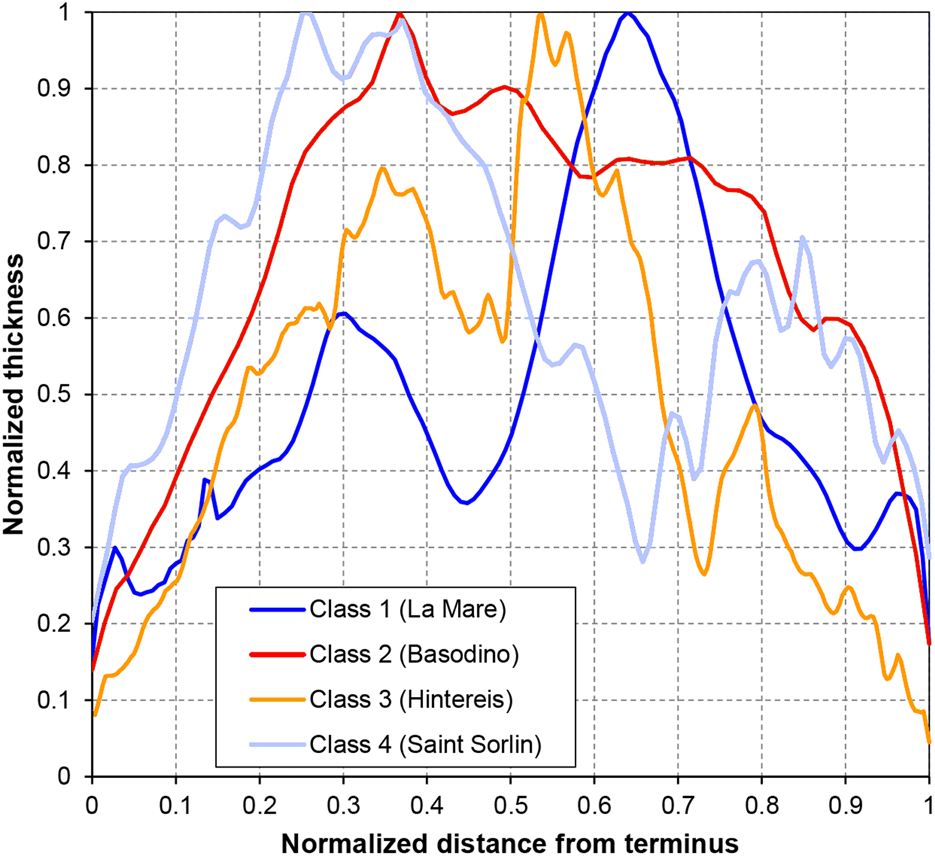
Fig. 6. Examples of normalised ice thickness vs normalised distance from the terminus, representing the four ITI classes of Sample B glaciers.
Similarly, glaciers with an uneven or undulating glacier bed are more prone to disintegration when getting thinner and are thus more vulnerable than glaciers with a more constantly flat or steep bedrock profile (Fig. 7a). We have manually classified glaciers as highly vulnerable if they have one or more large breaks in slope, and less vulnerable if slope changes are minor or absent (Table 1). Slope changes were assessed qualitatively from 2-D elevation profiles extracted along the centre lines from the D1 DEM.

Fig. 7. Three mass-balance glaciers in the Italian Alps that show very different behaviour and vulnerability: (a) La Mare Glacier, where a bedrock step is separating the lower ablation zone and where a lake might form (photo, L. Carturan, 12 September 2018); (b) Montasio Glacier, which is heavily covered by debris, avalanche fed and shadowed by steep rock walls (photo, F. Cazorzi, 16 August 2012); (c) Fontana Bianca Glacier, whose imminent extinction led to the interruption of mass-balance observation in 2018 (photo, C. Oberschmied, Agenzia per la Protezione civile – Provincia Autonoma di Bolzano – Alto Adige, 18 July 2018).
4.2.5 Elevation range and hypsometric index (criteria 5 and 6)
The elevation range of a glacier affects its ability to maintain an accumulation area during years with strong melting. If the range is too small, all snow (and later also firn) might melt away up to the highest elevations, resulting in a surface lowering and strong reduction of albedo, both further enhancing melt-down. Considering the histogram of elevation range values, we have used steps of 300 m to assign vulnerability classes 1 to 4 (Table 1).
The hypsometric distribution of area vs altitude is well recognised as an important control of glacier response to climatic changes because, in combination with a mass-balance gradient, it regulates the imbalance between net accumulation and ablation in response to ELA fluctuations (Furbish and Andrews, Reference Furbish and Andrews1984). We calculated a Hypsometric Index (HI) according to Jiskoot and others (Reference Jiskoot, Curran, Tessler and Shenton2009), with HI values lower than −1.5 indicating ‘top-heavy’ glaciers, with a large fraction of their area at high elevation and lower vulnerability (class 1) compared to the ‘bottom-heavy’ glaciers, with HI > 1.5 and most of their area lying at low elevation (class 4). Classes 2 and 3 have been assigned to values in-between (Table 1). Note that HI refers only to glacier area and elevation whereas ITI refers to ice thickness.
4.2.6 AAR sensitivity and observed AAR values (criteria 7 and 8)
The AAR sensitivity in the accumulation area is derived from the hypsometric curve, and expresses the change in the size of the accumulation area in response to a unit change in ELA. This variable accounts for the shape of the upper part of the glacier (flat or steep) and its effects in the preservation of an accumulation area following a possible ELA rise. Resulting values range from 0 to 1 that are assigned to classes 1 to 4 according to Table 1. A similar approach was used by Paul and others (Reference Paul2007) to model future glacier extents from a prescribed shift of the ELA and specific balanced-budget AAR values.
Because the AAR is strongly related to the annual mass balance of a glacier, average AAR values observed over a sufficiently long time period indicate the vulnerability of a glacier, assuming unchanged atmospheric conditions. Unlike variables derived from glacier geometry, the AAR enables accounting for regional climatic factors. For example, glaciers receiving high amounts of snowfall might benefit from a larger remaining snow cover despite their less favourable elevation range. The mean 2004–2013 AAR ($\overline {{\rm AAR}}$ ) was used for classifying glaciers from highly vulnerable ($\overline {{\rm AAR}}$
 < 0.1) to resilient ($\overline {{\rm AAR}}$
 > 0.5). In the case AAR values have not been reported for individual glaciers of Sample B (for Sample C they are complete), we have used the satellite-derived SCF as a proxy for the AAR (Fig. 8).

Fig. 8. End of summer snow cover as mapped from Landsat TM in 1985 (grey and white) and from Landsat OLI in 2015 (grey) using the method presented by Rastner and others (Reference Rastner2019). Image source: Copernicus Sentinel data 2015.
4.2.7 Avalanche, shadowing and debris cover (criterion 9)
Glaciers located under topographically favourable conditions may benefit from increased snow accumulation by avalanches and decreased ablation due to terrain shadowing. These are generally small glaciers lying at the bottom of steep rock walls in high-relief areas, which during deglaciation tend to persist and decouple from regional temperature fluctuations (e.g. Kuhn, Reference Kuhn1995; DeBeer and Sharp, Reference DeBeer and Sharp2009; Grünewald and Scheithauer, Reference Grünewald and Scheithauer2010; Carturan and others, Reference Carturan2013b). Additionally, debris cover reduces surface melt (e.g. Evatt and others, Reference Evatt2015; Rounce and others, Reference Rounce, King, McCarthy, Shean and Salerno2018) and thus reduces the vulnerability of glaciers with low-lying tongues or a small elevation range. We have grouped all three processes into one index because they tend to occur jointly and exhibit a similar forcing on mass balance, defining four classes of vulnerability that have been assessed qualitatively. Low vulnerability (class 1) is assigned to glaciers that are strongly shaded, covered by debris in their ablation area and mostly fed by avalanches (see e.g. the Montasio Glacier in Fig. 7b); high vulnerability (class 4) is inferred where these processes are absent and intermediate vulnerability is assigned to glaciers where they are of very local importance (class 3) or affect less than half of the glacier surface (class 2).
4.3 Correlation analysis
A correlation analysis was carried out to reveal major dependencies among variables expressing recent glacier behaviour, geometric adjustment and morphology. This analysis should provide a quantitative check of assumptions made in the selection of criteria for the combined GVI, and ease the interpretation of results. A correlation matrix was generated using the XLSTAT add-on for Microsoft Excel 2013. Variables expressing recent glacier behaviour are the mean annual balance and mean AAR in the period from 2004 to 2013; geometric adjustments in the same period are characterised by % area change and perimeter change, separating areas above and below the median elevation; glacier morphology in early 2000s is expressed by mean elevation, median elevation, mean exposure, mean slope, elevation range (see Section 4.1), HI and AAR sensitivity (see Section 4.2).
4.4 Mass-balance time series (Sample C)
Mass-balance observations of Sample C, covering a common period of 50 years, were analysed in detail to identify long-term trends and peculiarities in glacier behaviour. In particular, we analysed (i) variability in annual mass balances, (ii) individual mass balance departures from the mean of the remaining glaciers and (iii) cumulative mass-balance departures. The latter might indicate possible mass-balance regime shifts from equilibrium response due to down-wasting, with an increasing impact of non-climatic controls on glacier mass balance. To obtain a better visual impression of the mass-balance variability for (ii), single-year values are presented in combination with a centred 5-year moving average.
5. Results
5.1 Topographic analysis
The mass-balance glaciers analysed in this study (Sample B) vary in size from ice bodies smaller than 0.1 km2 (Pizol and Schwarzbach glaciers in Switzerland), to valley glaciers larger than 10 km2, reaching a maximum area of 17.2 km2 for Pasterze Glacier (Austria, Table S1). Overall, the frequency distribution of glacier sizes of Sample B is skewed towards larger area classes, compared to Sample A (Fig. 9). This is more evident considering frequency distributions by count (Fig. 9a) than by area (Fig. 9b). Hence, compared to the total sample of glaciers in the Alps (A) the sample of mass-balance glaciers (B) has relatively more of the larger glaciers included. This might seem surprising, but it directly results from the high number of glaciers smaller than 0.5 km2 in Sample A.

Fig. 9. Frequency distribution by count (left column) and area (right column) of glaciers of samples A and B, for classes of area (a, b), elevation range (c, d), mean elevation (e, f), slope (g, h) and aspect (i, l).
There is higher agreement in the frequency distributions of samples A and B when considering other morphometric variables. Their distribution is fairly similar and thus representative of the glaciers in the Alps. Sample B glaciers have a slightly higher elevation range (Figs 9c, d), lower mean elevation (Figs 9e, f) and lower slope (Figs 9g, h). The aspect distribution of Sample A is also well represented, with northern exposures prevailing in number for both samples (Fig. 9i). The area frequency distribution of aspect classes (Fig. 9l) show lower agreement, due to the presence of large glaciers exposed to the East in Sample B (e.g. Pasterze, Malavalle and Hintereis).
The lowest HI values in Sample B are reached at Pasterze (−2.25), Kesselwand (−2.13), Lunga (−2.10) and Findelen (−2.05) glaciers. These glaciers have the majority of their area in the upper part of their elevation range, and according to Jiskoot and others (Reference Jiskoot, Curran, Tessler and Shenton2009) they are ‘very top heavy’. The highest values of HI are found at Saint Sorlin and Pizol (both 2.04) as well as Wurten (1.85) glaciers, which are ‘very bottom heavy’ because most of their area lies in the lowest portion of the elevation range. Samples B and C have mean HI values of −0.43 and −0.45, respectively, meaning that they are both globally ‘equidimensional’. The hypsometry of Sample C is therefore representative of Sample B, considering also that Sample C includes Kesselwand and Saint Sorlin glaciers, which are at the two extremes in the range of variability of HI.
The correlation analyses applied to Sample B (Table S2) highlight how the HI alone does not explain the recent behaviour of glaciers, because it is not significantly correlated with the mean AAR, mean annual balance or other variables expressing their geometric changes. Hypsometry, however, influences the AAR sensitivity per unit change of ELA (see also Shea and Immerzeel, Reference Shea and Immerzeel2016), which results in close relationship with variables related to mass balance and area shrinkage. The correlation coefficients suggest that larger glaciers with higher elevation range have a lower AAR sensitivity and higher mean AAR in the observation period, which is in turn correlated to mass balance, as expected.
5.2 Mass-balance time series
Arithmetically averaged mass-balance values (Fig. 10) exhibit a high year-to-year variability. Balanced or positive mass budgets are common between 1967 and 1984, but become increasingly negative from 1985 to present. The extreme value of −2.6 m in the hot summer of 2003 (Schär and others, Reference Schär2004) is the lowest on record. The standard deviation of reference glacier mass balances increases over the period of record, in particular after 2003, and is illustrated by the individual glacier mass-balance records (in grey).

Fig. 10. Mean and std dev. of annual balance values for the nine glaciers of Sample C from 1967 to 2013.
Departures from the mean mass balance of the reference glaciers in Sample C show common regional trends and deviations (Fig. 11). When considering the 5-year running means, two peaks of positive departures are observed at the reference glaciers in France, three in the Ötztal Alps and for Careser, while no clear maxima are observed at Gries, Silvretta and Sonnblick glaciers. Thereby, the timing of the two peaks about 1980 and 1995 of Saint Sorlin and Sarennes fit to the local minima for the three Ötztal glaciers and Careser. Such deviations in opposite directions indicate a marked difference in the mass-balance forcing between the western and the eastern Alps. Assuming that the temperature forcing is similar for all glaciers, regional precipitation variability might explain the differences (Schwarb and others, Reference Schwarb, Daly, Frey and Schär2001; Auer and others, Reference Auer2007). A closer look at the values reveals further, more glacier specific differences: whereas the mass-balance differences of Silvretta and Kesselwand (to some extent also Sonnblick and Vernagt) are generally above zero (i.e. their mass budgets are more positive than the mean), Gries and Hintereis are mostly negative (Hintereis is mostly positive after 2000), Saint Sorlin was about the mean before 1995 and always negative afterwards, and Sarennes and Careser have always mass-balance values below the mean. This indicates that the glaciers might react to a common regional forcing regarding mass-balance variability, but individual factors are responsible for the absolute values.
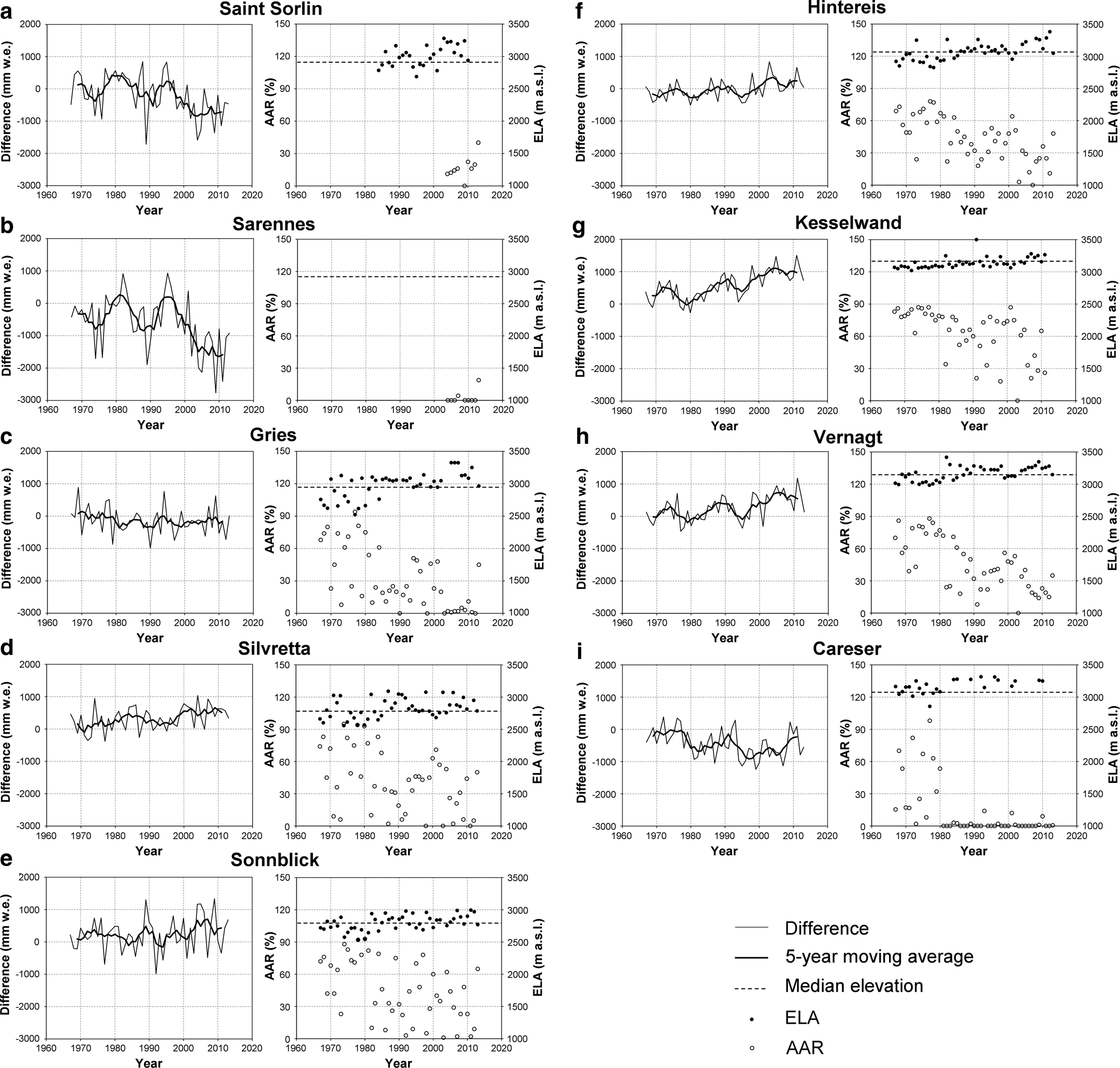
Fig. 11. Time series of the mass-balance differences of each glacier to the mean value of the other eight glaciers from Sample C. The right panel shows the respective series of annual ELA and AAR.
The AAR and ELA values for the reference glaciers provide additional context for long-term glacier change. In general, there is an increasing trend in ELA values, which mostly rose above the glaciers’ median elevations (dashed lines in Fig. 11) and reached the highest positions in the last decade. The AAR values show a large scatter and no clear trend for the glaciers with positive mass-balance deviations (Silvretta, Kesselwand and Sonnblick) and a clear negative trend for glaciers with negative deviations (Gries and Hintereis). Careser exhibits a switch in 1980 towards primarily zero AAR values. This coincides with ELAs above the median elevation of the glacier and increasingly negative mass-balance departures (Figs 11, 12a). From this we infer a regime shift in the mass balance for Careser. For Sarennes this shift can be derived from the mass-balance difference time series after 1995, when the negative differences started to steeply increase without recovering.
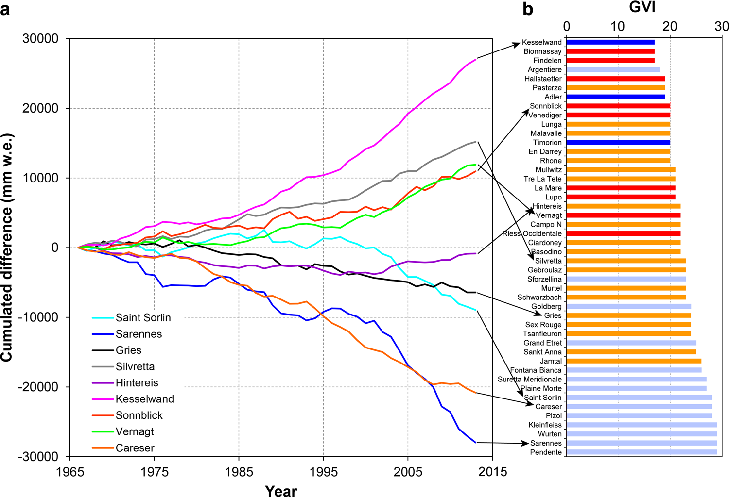
Fig. 12. Comparison of (a) time series of the cumulative mass-balance differences of each glacier to the mean value of the other eight glaciers from Sample C, and (b) the 46 glaciers of Sample B ranked for glacier vulnerability and colour-coded for elevation change pattern class (see Fig. 5 for colours).
5.3 Cumulative mass-balance differences
Regime shifts can be better observed in the cumulative mass-balance departures from the mean of Sample C (Fig. 12a). Cumulative departures are mostly positive for Kesselwand, Silvretta, Vernagt, Hintereis and Sonnblick glaciers, whereas increasingly negative departures are observed for Careser, Sarennes, Saint Sorlin and Gries glaciers. Increasingly negative cumulative departures begin in 1980 for Careser, 1995 for Sarennes, 2000 for Saint Sorlin and 1985 for Gries (though this is less pronounced). The differences between the glaciers are largely confirmed by the patterns of area and elevation changes. Although Careser, Sarennes and Saint Sorlin show large area and elevation losses at all elevations along with fragmentation (Fig. 3), shrinking of Vernagt, Sonnblick, Silvretta and Kesselwand is (in increasing order) restricted to the terminus region. Gries and Hintereis are in-between, i.e. substantial area and elevation losses occurred mostly in their ablation region, but tend to extend also higher up.
Cumulative differences in mass balance are also well reflected in the GVI classification (Fig. 12b). With only a few exceptions for glaciers with intermediate vulnerability, a high positive mass-balance deviation correlates with a low vulnerability index, and vice versa.
5.4 Vulnerability index
Figure 12b shows all glaciers of Sample B ordered by their GVI and colour-coded based on their class for the elevation change patterns (Fig. 5), with the three glaciers in class 1 that are among those with lowest GVI, and 10 out of the 14 glaciers in class 4 that have the highest GVI values. The Argentière and Pasterze glaciers are significant exceptions, because they experienced large thinning compared to other glaciers ranked with low vulnerability. These two glaciers theoretically benefit from a high elevation range, low AAR sensitivity in their upper zone and favourable overall hypsometry. However, they are also characterised by a complex morphology, the progressive detachment of several tributaries and by a large and relatively thick tongue, which is thinning rapidly. Dynamic adjustments are likely also involved in the calculated elevation change patterns, but are not easy to quantify or distinguish from surface lowering caused by ablation.
The number of glaciers that have been assigned to the individual classes is summarised in Table 2. The majority of glaciers lie in the intermediate vulnerability classes (2 or 3) for most criteria, however their distribution is clearly skewed towards high vulnerability for elevation change patterns, mean AAR and for the aggregated avalanche-shadowing-debris cover criterion, whereas they show lower vulnerability for area change, ice thickness and HIs. Based on observed series of AAR, the upper limit of the GVI for glacier survival seems to be ~25.
6. Discussion
6.1 Morphometric comparison
In general, the mass-balance glaciers of the Alps have been selected in order to detect inter-annual ELA fluctuations (i.e. high elevation range and low AAR sensitivity), minimise the influence of local topo-climatic effects (i.e. area large enough) and at the same time maximise ease of access and safety during field operations, as suggested for example by Kaser and others (Reference Kaser, Fountain and Jansson2003). These criteria highlight ‘ideal’ glaciers for direct mass-balance measurements, but are rarely met together at the same glacier. For this reason, mass-balance glaciers selected in the past few decades fulfil only parts of these requirements. As shown in Section 5.1, the topographic characteristics of glaciers in Sample B are fairly representative of all glaciers in the Alps, but are a little skewed towards larger glaciers, with higher elevation range, lower slope and lower mean elevation. An optimal representativeness of Sample B glaciers would have been possible only when using reasoned sampling schemes, based for example on the frequency distribution of glaciers for selected morphometric variables. However, the consistent application of sampling schemes is difficult if not impossible because glacier morphometry is dynamic and changing constantly. In this context, the recent efforts to include smaller glaciers, and also those fed by avalanches, in the monitoring network are valuable (e.g. Scotti and others, Reference Scotti, Brardinoni and Crosta2014; Huss and Fischer, Reference Huss and Fischer2016), although their time series are less directly related to changes in climatic conditions because non-climatic controls on glacier mass balance increase with decreasing glacier area (see e.g. the Montasio Glacier in Fig. 7; Carturan and others, Reference Carturan2013b).
6.2 Glacier behaviour and vulnerability
The analysis of the nine long-term mass-balance series in the Alps (Sample C) clearly suggest that, starting in the 1980s and becoming more evident in the 1990s and 2000s, local effects and/or feedbacks started to impact individual glaciers. This is revealed by the increasing spread among mass-balance series (Fig. 10) and by the regime shifts visible in the series of mass-balance difference and cumulated difference from the mean (Figs 11 and 12). Local differences tend to be less pronounced with less negative mass balances (Fig. 10), for example in the years 2001, 2010 and 2013, whereas they increase with more negative mass balances, for example in 2009 and 2011. A notable exception to this rule is the very warm year 2003, when widespread record-low mass balance was associated with comparatively low inter-glacier variability, possibly highlighting that above a certain summer temperature, local effects (e.g. precipitation variability and glacier morphometry) tend to decrease their importance.
Among the analysed morphometric characteristics and changes, the decadal scale elevation change pattern is probably the most effective indicator of a single glaciers ‘health’ and mass-balance development. This criterion has also been used by Pelto (Reference Pelto2010) in a qualitative manner as an indicator of glacier health. In fact, we note that the four elevation change pattern classes described in Section 4.2.3 are closely related to the mean AAR in the observation period, which is highly correlated with the mean annual balance (Table S2). Class 1 glaciers underwent small changes in area and shrunk exclusively near their terminus (e.g. Kesselwand in Fig. 3), keeping a rather large accumulation area ($\overline {{\rm AAR}}$ = 0.40 on average), even though they are not sustainable for current glacier extents. Class 2 glaciers show small elevation changes in their upper part compared to the ablation area, and are characterised by $\overline {{\rm AAR}}$
 values between 0.24 and 0.56 (0.37 on average) in the observation period (examples are Sonnblick and Vernagt in Fig. 3). Much smaller $\overline {{\rm AAR}}$
 values are found in class 3 glaciers (0.23 on average), where thinning is significant also in the upper part, and which is the most numerous in Sample B. This class represents also the larger glaciers of Sample A, that have flat tongues at low elevations suffering the most from the mass loss since 2000. Impressive examples of separated valley glacier tongues can be found everywhere in the Alps, e.g. Pasterze, Roseg, Damma, Trift and Grindelwald glaciers. Glaciers in class 4, with disequilibrium response, were mostly below the ELA in the observation period ($\overline {{\rm AAR}}$
 = 0.17 on average), because they are generally flat, located at low elevation and without topographic shadowing. In some cases they are also affected by unfavourable area and thickness distribution (i.e. bottom-heavy), such as Saint Sorlin in Figure 3. We observe that a classification of glacier behaviour and vulnerability is also possible with DEMs having a 30 m resolution, because the identification of the four main patterns has a limited dependence on correct absolute values of elevation change, and because class boundaries are not sharp and exceptions from the general picture of glacier retreat – such as the Belvedere Glacier (mini-)surge in 2001 (Haeberli and others, Reference Haeberli2002) – exist. A broad classification is feasible even without multi-temporal DEMs, for example using area change patterns (Section 4.2.2) that result from the combined effect of ice thickness and elevation change distributions.
Collectively, the proposed GVI classification is a promising tool for assessment of glacier vulnerability. The GVI is based on the evidence that topographic characteristics have an important impact on mass-balance development (Furbish and Andrews, Reference Furbish and Andrews1984; Paul and Haeberli, Reference Paul and Haeberli2008; DeBeer and Sharp, Reference DeBeer and Sharp2009; Benn and Evans, Reference Benn and Evans2010; Carturan and others, Reference Carturan2013c), and on the assumption that simple criteria, derived from remote-sensing imagery and DEMs, can be combined to classify glaciers according to their type of response and expected behaviour. This is also supported quantitatively by the results of our correlation analysis (Table S2 and Section 5.1), in particular for criteria expressing geometric adjustments and those related to glacier hypsometry (i.e. the elevation range and the AAR sensitivity per unit change of the ELA). Theoretically, low-resolution data should limit the applicability of the GVI for very small glaciers. Although the GVI has been developed for glaciers larger than ~0.5 km2, the results indicate that the index can also be applied to small glaciers (Fig. 12 and Table S1). This is likely due to the combination of multiple criteria.
The nine criteria used here for a determination of the GVI have not been weighted although one can certainly argue that some of them are more important than others. Moreover, some of them are similar (e.g. HI and AAR sensitivity) but are not combined. We have thus tested several other criteria combinations (see Supplementary material), and while there are some small differences, the overall ranking of glacier vulnerability is robust. Uncertainties related to input datasets (see Section 6.3) or subjectivity in class threshold assignments may affect single criteria, but tend to level out when combining all GVI criteria. The GVI is thus considered as a robust index to determine glacier vulnerability. The proposed combination of criteria exploits a wide range of available information but maintains a reasonable degree of simplicity.
6.3 Uncertainties
For this study we have applied several datasets (glacier outlines, DEMs, ice thickness, mass balance and snow cover) in various combinations. Each of the datasets has an uncertainty that has been neglected so far. The main reason is the limited impact these uncertainties have on the results of the GVI classification. This is in part due to the analysis of patterns, trends and indices rather than absolute values. The former are much more robust and are not expected to change substantially when using different datasets. For example, instead of the DEMs and glacier outlines used here one could have also used other DEMs and/or outlines from other dates (both spanning a decadal time period) to observe the same pattern and derive the same class assignment. This is due to sustained shrinkage of glaciers in the Alps since about 1985 (Paul and others, Reference Paul, Rastner, Azzoni, Diolaiuti, Fugazza, Bris, Nemec, Rabatel, Ramusovic, Schwaizer and Smiraglia2020).
The area change patterns might also be influenced by wrongly included seasonal snow in outlines O1 and O2, but this can be excluded here as summer months in 2003, 2006, 2013 and 2015 had been very hot and nearly all off-glacier snow had melted. Glacier extents for analysed years should thus be accurate and the derived change pattern realistic.
The elevation change pattern is derived from two DEMs (SRTM and TanDEM-X) with a well-known significant radar penetration in snow. For Careser and La Mare glaciers we have thus compared elevation changes derived from these DEMs (Fig. 13a) with those derived from subtracting two LIDAR DEMs acquired in 2003 and 2013 (Fig. 13b). Careser represents glaciers that lack firn and snow in their upper part since the 1980s, whereas La Mare is representative of glaciers in active retreat, with preserved snow and firn in their upper zone in the past few decades (Carturan and others, Reference Carturan2013a; Carturan, Reference Carturan2016). Although the general pattern of elevation change is very similar, absolute values show a stronger overall thinning for the LIDAR difference, in particular for the upper region of La Mare Glacier. Accordingly, La Mare is in class 2 in our study and would be in class 3 according to the LIDAR difference map, indicating that our classification is on the conservative side (i.e. smaller vulnerability). Considering that the distinction among the four patterns takes into account not only the absolute elevation changes but also their elevation dependence and variability, possible errors in glacier ranking due to radar penetration are limited to classes 2 and 3, as shown for La Mare Glacier. Assuming that all class 2 glaciers are wrongly classified and actually belong to class 3, as tested in a GVI experiment, lead to a vulnerability classification with the same results as in Figure 12.

Fig. 13. Comparison between annual elevation change rate from (a) SRTM DEM and TanDEM-X DEM (period 2000–13), and (b) LiDAR surveys (period 2003–13), on the two neighbouring Careser (top row) and La Mare (bottom row) glaciers in the Italian Alps.
The modelled ice thickness has an uncertainty of ~30% compared to results from other methods and GPR measurements, but this uncertainty is not related to a specific zone of the glacier (Linsbauer and others, Reference Linsbauer, Paul and Haeberli2012). In consequence, the impact on the index (ITI) should be small. Slope changes as well as combined local criteria (avalanches, shadowing and debris cover) have been derived qualitatively and are thus largely independent of DEM uncertainties. The elevation range, HI and AAR sensitivities are all derived from a DEM with uncertainties (GDEM2), but they do not really impact on the classes assigned here, i.e. we would get similar classes with another DEM.
Finally, the mean AAR values for Sample C glaciers are mostly derived from field measurements and should thus be robust. For the glaciers in Sample B, 30% of the values are derived from satellite data using the SCF proxy. Because the SCF values are expected to be larger than the AAR values, as satellite images were seldom acquired at the end of the ablation period, we did a comparison of SCF and AAR for several years and glaciers where both are available (Table 3). The comparison reveals that the generally small SCF overestimations tend to be compensated by underestimations due to SLC-off striping (ETM+ sensor after 2003) or shadows cast by clouds and rock walls, resulting in mean difference of zero and a standard deviation of 0.08.
Table 3. Comparison between field measured AAR and SCF derived by classification of late summer Landsat imagery for different years and several mass-balance glaciers in the Alps

The mean difference is 0.0 with a standard deviation of 0.08.
6.4 Future perspectives
Glaciers in the mass-balance monitoring network of the Alps (Sample B) are fairly representative of all other glaciers (apart from the rare largest ones), and they are similarly characterised by rapid down-wasting and eventual disappearance. Among Sample C glaciers, Sarennes is nearly extinct and Careser will likely follow shortly. The latter is still ~60 m thick in the eastern part, but there is a lake forming at the front that is likely to accelerate glacier wastage. Without these two glaciers, the average mass balance of Sample C would have been 0.23 m less negative in the period from 2000 to 2013 (−1.02 vs −1.25 m w.e.), whereas between 1967 and 1980 the two means were almost identical (0.063 vs −0.005 m w.e.). The high imbalance and nonlinear response of these two glaciers is therefore affecting significantly the glaciological mass-balance estimates from reference glaciers at the mountain range scale, and will result in a discontinuity in the time series when the two glaciers have vanished and/or will be replaced with glaciers having less negative mass-balance values.
There is a significant number of monitored glaciers in the Alps experiencing the same fate (Fig. 12). They were missing a significant accumulation area for a long time and after decades of strong mass loss they are considerably smaller, thinner and changed in shape compared to when measurements begun. In some cases (e.g. Sforzellina) negative feedbacks from increasing debris cover and avalanche contribution tend to preserve the residual ice bodies, but other glaciers are at the final stage of becoming extinct. This can lead to increased complexity in performing observations and also calculating reasonable glacier-wide mass balances from the remaining network of stakes (e.g. some elevation intervals might no longer be covered by ice). In 2018, for example, mass-balance measurements were discontinued on the Fontana Bianca Glacier (Fig. 7c, where they started in 1983), because of the rockfall danger and low regional representativeness.
It can also be assumed that the formation of pro-glacial lakes in overdeepenings of the glacier bed (e.g. Paul and others, Reference Paul, Kääb and Haeberli2007; Frey and others, Reference Frey, Haeberli, Linsbauer, Huggel and Paul2010; Emmer and others, Reference Emmer, Merkl and Mergili2015) will continue in the future (e.g. Linsbauer and others, Reference Linsbauer, Paul and Haeberli2012; Haeberli and others, Reference Haeberli, Linsbauer, Cochachin, Salazar and Fischer2016) and considerably enhance glacier retreat for numerous glaciers (e.g. Purdie and Fitzharris, Reference Purdie and Fitzharris1999). This effect has only indirectly been considered in the GVI (e.g. via the criteria slope changes and HI) but might be in particular important for larger valley glaciers with flat tongues. However, pro-glacial lake formation depends on the (unknown) details of the bed topography. Moreover, lakes might impact on glacier retreat only for a limited amount of time as overdeepenings are often locally constrained. We have thus not considered it in our simplified index calculation.
Combined indexes such as the GVI might be used for early detection of glaciers at risk of extinction in the near-future and possible candidates with higher chance to survive, to be evaluated as possible replacements for currently monitored glaciers or other long-term investigations. Moreover, the index can be used to determine if the mass balance of a glacier will be impacted sooner or later by factors other than climate. This information can be used to develop a longer-term perspective of mass-balance measurements for the currently selected glaciers, but also to pre-select such glaciers in other regions of the world. Test of GVI versions with a reduced number of criteria indicate that they might also be applied reliably in the case of reduced data availability, or possibly in a semi-automatic fashion over a large number of glaciers. In particular, we obtained a classification that is very similar to the GVI presented in Figure 12 when removing all criteria dependent on DEM availability (i.e. elevation change pattern, HI, ITI and AAR sensitivity in the accumulation area), or all criteria that require multi-temporal observations (ACI, $\overline {{\rm AAR}}$ and elevation change pattern). Comparing the GVI with single criteria revealed that good results can be achieved using the elevation change pattern alone, and very good results are obtained using the AAR sensitivity in the accumulation area (resulting in no arrow crossings when connecting the nine cumulative mass-balance differences to the glaciers ranked for GVI).
In hind cast, it might also be possible to decide about the removal of specific glaciers from the sample of reference glaciers that is used for region-wide mass-balance averaging. However, to be fully aware of a possible regime shift (as shown for the Careser Glacier) and the impacts of climatic variability on such glacier remnants, it is important to continue and report field measurements on the remaining ice as long as possible.
The removal/replacement of existing series is not trivial. First, class 4 glaciers contribute an important part of the climatic response of the glacier system in the Alps, and their (sudden) exclusion would imply a step change in mountain range mass-balance estimates (unless the non-climatic response is identified and adjusted in its early stages), and a spurious shift towards a less negative mean budget. However, current approaches to extrapolate measured mass balances to a larger sample (Zemp and others, Reference Zemp2019) are less dependent on the absolute values (that are taken from geodetic measurements) than on their temporal variability. The latter seems to be synchronous for some time, even if a glacier is close to disappearance. Hence, using mass-balance variability is less impacted by lingering glacier disappearance than absolute values. However, one has to be aware that over elongated mountain ranges such as the Alps, where different sub-regions can experience opposite effect from the same atmospheric circulation patterns (in particular regarding precipitation amounts), large differences in the mass-balance variability exist. The two glaciers in the French Alps have basically the opposite variability (deviation from the mean) compared to the three in the Ötztal Alps, Careser and Sonnblick (Fig. 11). Just using either group would thus give a different picture of the regional mass-balance variability. The common climatic forcing that has been proposed for the glaciers in the Alps (e.g. Vincent and others, Reference Vincent2017) is thus potentially modified by regional variability in precipitation and cloud cover (Quadrelli and others, Reference Quadrelli, Lazzeri, Cacciamani and Tibaldi2001; Schmidli and others, Reference Schmidli, Schmutz, Frei, Wanner and Schär2002; Brunetti and others, Reference Brunetti2006, Reference Brunetti2009; Auer and others, Reference Auer2007).
7. Conclusions
In this study we have analysed the morphometric and mass-balance characteristics of the mass-balance glaciers that are currently measured in the Alps. We developed an index (GVI) to determine their resilience to climatic changes. The investigation was motivated by the loss of mass-balance glaciers and the need to replace them with glaciers that are more resilient in good time. The GVI is derived from glacier outlines and a DEM (e.g. breaks in slope and HI) in combination with criteria derived from multi-temporal data (e.g. area and elevation changes and snow cover) and modelling (ice thickness distribution). The index assignment was developed for the Alps but can be adjusted to other regions. Overall, we found a very good agreement between the GVI and the ranked cumulative deviations of the mass balance from the nine glaciers with long-term measurements, providing confidence in its wider applicability. For the next few decades the GVI can also be used when searching for glaciers that might replace in the future those in the current selection or new ones.
For a few glaciers (Careser, Sarennes and Saint Sorlin) we identified regime shifts in their mass-balance time series indicating the increasing impact of non-climatic controls on their mass balance, and likely leading to too negative values of the Alpine wide average afterwards (by ~0.2 m w.e.). Just removing them from the sample is, however, not straight forward as these shifts can only be identified in hindsight. This requires continuing measurements also on disintegrating glaciers for several years. At best, such measurements are performed in parallel with the replacement glacier to learn about the differences of the new time series. The direct comparison of the mass-balance differences reveals interesting deviations and common patterns on a regional scale, indicating that regional differences under meteorological conditions (e.g. precipitation amounts) might be responsible for it. Overall, the glaciers currently selected for mass-balance measurements (Sample B) reflect the key geomorphologic characteristics of the entire sample very well, but are biased towards somewhat larger glaciers in relative terms. Despite this good representativeness, very large glaciers (e.g. Aletsch, Gorner and Unteraar) are missing and their strong mass loss at low elevations (though having a high albedo or thick debris cover) is not well captured by the current sample. Unconsidered characteristics such as response times or lake formation might have to be added when choosing a new observation site.
Supplementary material
The supplementary material for this article can be found at https://doi.org/10.1017/jog.2020.71
Acknowledgements
L.C. acknowledges funding from the University of Padova Senior Research Grant: ‘Impact of climatic fluctuations on snow- and ice-dominated alpine watersheds: effects on the cryosphere and hydrology’. The 2006–2007 outlines of Italian glaciers data were furnished by Maria Cristina Salvatore (project of strategic interest CNR-NEXTDATA, PI Antonello Provenzale CNR-IGG, WP 1.6, Carlo Baroni UNIPI). P.R. and F.P. acknowledge funding from the ESA project Glaciers_cci (4000109873/14/I-NB) and the Copernicus Climate Change Service (C3S) that is funded by the European Union and implemented by ECMWF. The TanDEM-X DEM has been acquired by the TerraSAR-X/TanDEM-X mission and is provided by DLR (DEM_GLAC1823). We also thank Matthias Huss from the ETH Zurich for providing the ice thickness distribution data for the glaciers in the Alps, and Wilfried Haeberli and Michael Zemp for their suggestions.


 Open access