


1. Introduction
The motion of particles in a fluid is one of the central problems in fluid mechanics, across many scales. The hydrodynamic drag force exerted by the fluid on the particles is the fundamental quantity that dictates the motion. Applications include the sedimentation of synthetic entities, the swimming of biological microorganisms (see Wang & Ardekani Reference Wang and Ardekani2012; Wei et al. Reference Wei, Dehnavi, Aubin-Tam and Tam2019, Reference Wei, Dehnavi, Aubin-Tam and Tam2021; Redaelli et al. Reference Redaelli, Candelier, Mehaddi, Eloy and Mehlig2023), blood flows (see Ku Reference Ku1997), peristaltic pumping (see Shapiro, Jaffrin & Weinberg Reference Shapiro, Jaffrin and Weinberg1969), microfluidic flows (see Dincau, Dressaire & Sauret Reference Dincau, Dressaire and Sauret2020) and Brownian motion at short times (see Felderhof Reference Felderhof2005; Mo & Raizen Reference Mo and Raizen2019). At small Reynolds number, while the steady, bulk, Stokes drag force exerted on a translating sphere is well known, addressing further the transient contributions is more intricate – even though the implications of such effects are potentially numerous.
For an isolated spherical particle with radius  $R$ translating in a viscous liquid at velocity $\boldsymbol {V}$, the bulk drag force $\boldsymbol {F}$ at small Reynolds number is given by the Basset–Boussinesq–Oseen (BBO) expression (see Basset Reference Basset1888; Gatignol Reference Gatignol1983; Maxey & Riley Reference Maxey and Riley1983; Lovalenti & Brady Reference Lovalenti and Brady1993; Landau & Lifshitz Reference Landau and Lifshitz1987)
 \begin{equation} \boldsymbol{F}={-}6{\rm \pi}\eta R\boldsymbol{V} - 6R^2\sqrt{{\rm \pi}\rho \eta}\int_{-\infty}^t \frac{1}{\sqrt{t-\tau}}\,\frac{\mathrm{d} \boldsymbol{V}}{\mathrm{d}\tau}\,\mathrm{d}\tau - \frac{2{\rm \pi} \rho R^3}{3}\,\frac{\mathrm{d}\boldsymbol{V}}{\mathrm{d}t}, \end{equation}
where  $\rho$ and $\eta$ are the density and dynamic viscosity of the viscous liquid, respectively. The right-hand side of this equation includes three terms successively: a Stokes viscous force, a Basset memory term, and an added-mass term. The Basset force originates from the diffusive nature of vorticity within the unsteady Stokes equation, and the added-mass force can be interpreted as an inertial effect due to the displaced fluid mass. Equation (1.1) provides a good description of particle dynamics in a large variety of particle-laden and multi-phase flows, as long as the particle Reynolds number is small (see Balachandar & Eaton Reference Balachandar and Eaton2010).
Nevertheless, the effect of nearby solid boundaries on the unsteady drag is still an open question. The canonical situation is that of an immersed sphere oscillating near a planar rigid surface. Some asymptotic expressions of the drag in the large-distance limit have been derived recently, by using a point-particle approximation together with the method of images (Felderhof Reference Felderhof2005, Reference Felderhof2012; Simha, Mo & Morrison Reference Simha, Mo and Morrison2018), or by using low- or high-frequency expansions of the unsteady Stokes equations (Fouxon & Leshansky Reference Fouxon and Leshansky2018). However, theoretical descriptions of the confined limit, i.e. where the sphere is in close proximity to the surface, are scarce. We thus aim here to investigate the unsteady drag, in the full spatial range from bulk to confinement, by combining numerical simulations, asymptotic calculations and colloidal-probe atomic force microscopy (AFM) experiments.
The AFM colloidal-probe methods and their surface force apparatus analogues were first introduced in the 1990s in order to measure molecular (e.g. electrostatic or van der Waals) interactions between surfaces (see Butt Reference Butt1991; Ducker, Senden & Pashley Reference Ducker, Senden and Pashley1991; Butt, Cappella & Kappl Reference Butt, Cappella and Kappl2005). Recently, these methods have been extended and used to study flow under micro-to-nanometric confinement, e.g. near soft (see Leroy & Charlaix Reference Leroy and Charlaix2011; Leroy et al. Reference Leroy, Steinberger, Cottin-Bizonne, Restagno, Léger and Charlaix2012; Villey et al. Reference Villey, Martinot, Cottin-Bizonne, Phaner-Goutorbe, Léger, Restagno and Charlaix2013; Guan et al. Reference Guan, Charlaix, Qi and Tong2017; Zhang et al. Reference Zhang, Arshad, Bertin, Almohamad, Raphael, Salez and Maali2022) or capillary interfaces (see Manor et al. Reference Manor, Vakarelski, Tang, O'Shea, Stevens, Grieser, Dagastine and Chan2008; Vakarelski et al. Reference Vakarelski, Manica, Tang, O'Shea, Stevens, Grieser, Dagastine and Chan2010; Manica, Klaseboer & Chan Reference Manica, Klaseboer and Chan2016; Maali et al. Reference Maali, Boisgard, Chraibi, Zhang, Kellay and Würger2017; Wang et al. Reference Wang, Zeng, Alem, Zhang, Charlaix and Maali2018; Bertin et al. Reference Bertin, Zhang, Boisgard, Grauby-Heywang, Raphaël, Salez and Maali2021), using complex fluids (see Comtet et al. Reference Comtet, Chatté, Nigues, Bocquet, Siria and Colin2017a,Reference Comtet, Niguès, Kaiser, Coasne, Bocquet and Siriab, Reference Comtet, Lainé, Nigues, Bocquet and Siria2019), or to measure the friction at solid–liquid interfaces (see Cottin-Bizonne et al. Reference Cottin-Bizonne, Barrat, Bocquet and Charlaix2003; Maali, Cohen-Bouhacina & Kellay Reference Maali, Cohen-Bouhacina and Kellay2008; Cross et al. Reference Cross, Barraud, Picard, Léger, Restagno and Charlaix2018), and electrohydrodynamic effects (see Liu et al. Reference Liu, Zhao, Mugele and van den Ende2015, Reference Liu, Klaassen, Zhao, Mugele and Van Den Ende2018; Zhao et al. Reference Zhao, Zhang, van den Ende and Mugele2020; Rodríguez Matus et al. Reference Rodríguez Matus, Zhang, Benrahla, Majee, Maali and Würger2022). More specifically, for dynamic colloidal AFM measurements, a micron-size spherical colloidal probe is placed in a viscous fluid, in the vicinity of a surface, with a sphere–wall distance  $D$. Then the probe is driven to oscillate without direct contact, via either acoustic excitation or thermal noise. The force exerted on the sphere is inferred from the colloidal motion, through the cantilever's deflection, which allows us to extract specific information on the confined surfaces or fluid properties. We point out that other experimental techniques were used to probe the bulk streaming flow around an oscillating sphere at finite Reynolds numbers, like particle visualization techniques (Kotas, Yoda & Rogers Reference Kotas, Yoda and Rogers2007; Otto, Riegler & Voth Reference Otto, Riegler and Voth2008) and optical tweezers (Bruot et al. Reference Bruot, Cicuta, Bloomfield-Gadêlha, Goldstein, Kotar, Lauga and Nadal2021).
If the typical angular frequency of the flow is  $\omega$, then the vorticity diffuses on a typical distance $\delta \sim \sqrt {\eta /(\rho \omega )}$ called the viscous penetration length. The dynamic force measurements are usually restricted to low Reynolds numbers and low probing frequencies, and to the confined regime where $D\ll R$. In such a case, the penetration length is large, the flow is located mainly in the confined fluid layer, it is purely viscous and quasi-steady, and the lubrication theory holds (see Reynolds Reference Reynolds1886; Leroy & Charlaix Reference Leroy and Charlaix2011). Consequently, in all the above examples, the fluid inertial effects are disregarded in the analysis of the measured hydrodynamic force. This omission is justified by the low Reynolds number, expressed as $Re=\rho \omega A R/\nu$, where $A$ represents the amplitude of the probe's oscillation, and where $\nu =\eta /\rho$ is the kinematic viscosity of the fluid. However, when the colloidal probe oscillates at high frequencies, the penetration depth $\delta$ might become comparable to, and even smaller than, the characteristic length scale of the flow. Thus unsteady effects may become important (see Clarke et al. Reference Clarke, Cox, Williams and Jensen2005), even though $Re$ might remain small. The relevant dimensionless number to characterize the crossover to such a regime is the Womersley number $Wo = R \sqrt {\omega / \nu }$, the square of which corresponds to the ratio between the typical diffusion time scale $R^2/\nu$ and the period of the oscillation. Unsteady inertial effects should be predominant when it takes more time for the vorticity to diffuse than for the sphere to oscillate, i.e. $Wo > 1$. In such a situation, the hydrodynamic force exerted on the sphere not is only a viscous lubrication drag, but also contains contributions due to the unsteady fluid inertia, which were studied partly in previous works (see El-Kareh Reference El-Kareh1989; Sader Reference Sader1998; Benmouna & Johannsmann Reference Benmouna and Johannsmann2002; Clarke et al. Reference Clarke, Cox, Williams and Jensen2005; Devailly et al. Reference Devailly, Bouriat, Dicharry, Risso, Ondarçuhu and Tordjeman2020).
The paper is organized as follows. In § 2, we introduce the experimental method of thermal noise AFM and present the typical experimental results. We show that as the distance to the wall is reduced, the resonance frequency increases for low Womersley numbers but decreases for high Womersley numbers. In contrast, the dissipation increases monotonically with decreasing distance for all Womersley numbers. In order to rationalize the results, in § 3, we compute the hydrodynamic drag force in terms of added mass and dissipation, in the asymptotic limit of large distance, and we perform a detailed calculation in the low-Womersley-number limit using the Lorentz reciprocal theorem. Furthermore, a finite-element method is employed to obtain the full numerical solution in all regimes. Finally, the experimental, theoretical and numerical results are summarized and compared in § 4. Mainly, the variation of the resonance frequency is rationalized by the change of the effective mass with distance and Womersley number.
2. Experiments
2.1. Colloidal-probe AFM set-up
A schematic of the experimental system is shown in figure 1(a). A borosilicate sphere (MOSci Corporation, radius  $R=27 \pm 0.5 \ \mathrm {\mu } {\rm m}$) is glued (Epoxy glue, Araldite) to the end of an AFM cantilever (SNL-10, Brukerprobes), and located near a planar mica surface. The cantilever stiffness $k_{c}=0.68\pm 0.05 \ {\rm N}\ {\rm m}^{-1}$ is calibrated using the drainage method proposed by Craig & Neto (Reference Craig and Neto2001). The experiments were performed using an AFM (Bruker, Dimension3100) in three different liquids, i.e. water, dodecane and silicone oil, whose densities and dynamic viscosities are $1000$ kg m $^{-3}$ and 1 mPa s, $750$ kg m $^{-3}$ and 1.34 mPa s, and $930$ kg m $^{-3}$ and 9.3 mPa s, respectively, at room temperature. The sphere–wall distance $D$ was controlled by an integrated stage step motor. Each separation distance was adjusted by displacing the cantilever vertically using the step motor with precision in position <0.1 $\mathrm {\mu }$m. The zero distance was determined as the point where the deflection signal changed sharply due to the solid–solid contact of the probe with the wall. The cantilever's deflection produced by thermal and hydrodynamic forces acting on the probe was acquired directly using an analogue to digital (A/D) acquisition card (PCI-4462, NI, USA) with sampling frequency 200 kHz. The amplitude of the thermal fluctuation of the probe remained smaller than $\sim$1 nm, in all the experiments.

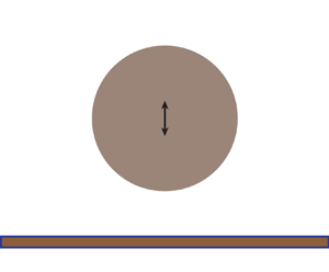
Figure 1. Schematics of the system. A borosilicate sphere with radius  $R$ is glued at the end of an AFM cantilever, and fluctuates thermally within a viscous liquid and near a mica substrate, with a distance $D$ between the sphere and the substrate. The sphere and mica surfaces are denoted as $\mathcal {S}_0$ and $\mathcal {S}_{w}$, respectively.
2.2. Confined thermal dynamics
The time-dependent position of the spherical probe is denoted  $Z(t)$. For a given sphere–wall distance $D$, the probe dynamics can be modelled by a forced harmonic oscillator (see Jai, Cohen-Bouhacina & Maali Reference Jai, Cohen-Bouhacina and Maali2007; Kiracofe & Raman Reference Kiracofe and Raman2011; Maali & Boisgard Reference Maali and Boisgard2013), as
 \begin{equation} m_\infty \ddot{Z}+ \gamma_\infty \dot{Z} + k_{c} Z = F_{th} + F_{int}, \end{equation}
where  $m_\infty$ is the effective mass of the probe in the bulk, and $\gamma _\infty$ is the bulk damping coefficient. These two coefficients correspond to the free dynamics of the probe far from the surface, and can thus be obtained by measuring the resonance properties of the AFM probe in the far field, as shown below. Besides the elastic restoring force by the cantilever of stiffness $k_{c}$, and in the absence of conservative forces (e.g. van der Waals or electrostatic forces), the two main forces acting on the sphere along the $z$ direction are the random thermal force $F_{th}$ and the hydrodynamic interaction force with the wall $F_{int}$. The latter corresponds to the deviation of the hydrodynamic drag with respect to the bulk drag force and depends on the sphere–wall distance.
Taking the Fourier transform of (2.1), we find
 \begin{equation} - m_\infty \omega^2 \tilde{Z} + {\rm i}\omega \gamma_\infty \tilde{Z} + k_{c} \tilde{Z} = \tilde{F}_{th} + \tilde{F}_{int}, \end{equation}
where  $\tilde {f}(\omega ) = ({1}/{2{\rm \pi} })\int _{-\infty }^{\infty } \mathrm {d}t\,f(t) \,{\rm e}^{-{\rm i} \omega t}$ is the Fourier transform of the function $f(t)$. The real and imaginary parts of $\tilde {F}_{int}$ correspond to an inertial force and a dissipative force, respectively, that can be recast into
 \begin{equation} \tilde{F}_{int} = m_{int} \omega^2 \tilde{Z} - {\rm i}\omega\gamma_{int} \tilde{Z}, \end{equation}
where  $m_{int}$ and $\gamma _{int}$ are the wall-induced variations of the effective mass and dissipation coefficient. For the sake of simplicity, we neglect in the following the possible frequency dependencies of $m_{int}$ and $\gamma _{int}$. With this main assumption, and injecting (2.3) into (2.2), the probe's motion follows a thermally forced harmonic oscillator dynamics with spring constant $k_{c}$, effective damping coefficient $\gamma \equiv \gamma _\infty + \gamma _{int}$, and effective mass $m \equiv m_\infty + m_{int}$. For the latter problem, one can then derive the one-sided power spectral density $S(\omega ) \equiv 2 \langle \vert \tilde {Z}(\omega ) \vert ^2 \rangle$, as
 \begin{equation} S(\omega) = \frac{2 \langle \vert F_{th} \vert ^2 \rangle / (m^{2}\omega_0^4)}{\left[1-\left(\dfrac{\omega}{\omega_0}\right)^2 \right]^2+\left(\dfrac{\omega}{\omega_0 Q} \right)^2} = \frac{2k_{B}T / ({\rm \pi} Q m \omega_0^3)}{\left[1-\left(\dfrac{\omega}{\omega_0} \right)^2 \right]^2+\left(\dfrac{\omega}{\omega_0 Q} \right)^2} , \end{equation}
where  $\langle \cdot \rangle$ denotes the ensemble average, $k_{B}T$ is the thermal energy, $\omega _0 = \sqrt {k_{c}/m}$ is the resonance angular frequency, and $Q=m\omega _0/\gamma$ is the quality factor. The second equality in (2.4) is obtained by using the correlator of the noise $\langle F_{th}(t)\,F_{th}(t') \rangle = 2 \gamma k_{B}T \delta _{D}(t-t')$, where we assumed a white noise through the Dirac distribution $\delta _{D}$ , and where we invoked the fluctuation–dissipation theorem to set the amplitude of the noise. The experimental power spectral densities are fitted by the function (Honig et al. Reference Honig, Sader, Mulvaney and Ducker2010; Bowles, Honig & Ducker Reference Bowles, Honig and Ducker2011)
 \begin{equation} S(\omega) = \frac{c_1}{\left[1-\left(\dfrac{\omega}{\omega_0} \right)^2 \right]^2+\left(\dfrac{\omega}{\omega_0 Q} \right)^2} + c_2, \end{equation}
where  $\omega _0$ and $Q$ are the key adjustable parameters indicating the position and width of the resonance, and $c_1$ and $c_2$ are unimportant extra parameters allowing us to accommodate for potential spurious experimental offset and/or prefactor.
2.3. Power spectral density
Figure 2 displays the power spectral densities for probes immersed in dodecane or silicone oil (water was employed as well, but the similar results are not shown here), and for a variety of sphere–wall distances. A well-defined peak can be observed for each spectrum, indicating the fundamental resonance. The resonance properties are well described by the damped harmonic oscillator model above. The largest sphere–wall distance ( $D=100\ \mathrm {\mu }{\rm m}$) corresponds to nearly four times the sphere radius, so that the hydrodynamic interactions between the probe and the wall can be neglected. At such distances, the bulk resonance frequency $\omega _0^\infty = \sqrt {k_{c}/m_\infty }$ and bulk quality factor $Q_\infty = m_\infty \omega _0^\infty /\gamma _\infty$ are extracted from the fitting procedure, giving respective values $7070\pm 5$ Hz and $3.3\pm 0.1$ in dodecane, and $5320\pm 5$ Hz and $1.3\pm 0.1$ in silicone oil. In the more viscous fluid (silicone oil), the resonance is broader since the dissipation is larger, as expected. Also, in both liquids, we observe that the resonance is broader as the sphere gets closer to the hard wall, which indicates that the near-wall dissipation is larger as compared to the bulk situation, as expected too. Besides, and interestingly, the bulk resonance frequency changes significantly from silicone oil to water ( $\approx$20 % difference in $\omega _0^\infty$, which means $\approx$50 % difference in effective mass), although the liquid density is similar (less than 10 % difference). Hence the effective mass depends on the viscosity of the ambient fluid in a non-trivial way. Moreover, the resonance frequency depends on the sphere–wall distance.

Figure 2. Experimental power spectral densities in arbitrary units (a.u.), for the colloidal probe's vertical position, in (a) dodecane and (b) silicone oil, for various sphere–wall distances as indicated. The curves are shifted vertically for clarity. The solid lines show the best fits to the damped harmonic oscillator model, using (2.5).
To be quantitative, the fitted values of the resonance frequency  $\omega _0$ and the quality factor $Q$ are shown in figure 3 as functions of the normalized separation distance $D/R$, for the three liquids studied. Intriguingly, we observe an increase of the resonance frequency in silicone oil near the wall as compared to the bulk resonance frequency (figure 3a), and a corresponding decrease in dodecane (figure 3c) and water (figure 3e). We point out that the sphere–wall distances in the present experiments are large enough ( $D>0.5\ \mathrm {\mu } {\rm m}$) so that molecular interactions (e.g. electrostatic or van der Waals forces) can be neglected safely. Therefore, the changes in resonance frequency observed here should result only from hydrodynamic contributions. The next section aims to model this intricate behaviour.

Figure 3. Resonance frequency  $\omega _0/(2{\rm \pi} )$ (blue dots) and quality factor $Q$ (orange dots) of the normal mode of the colloidal AFM probe as a function of dimensionless sphere–wall distance $D/R$. The dashed lines represent the resonance frequencies and quality factors calculated by (4.3) and (4.4), respectively, without adjustable parameter. (a,b) Results for silicone oil ( $\eta = 9.3$ mPa s, $\rho = 930$ kg m $^{-3}$), with squared Womersley number $Wo^2 =2.4$. (c,d) Results for dodecane ( $\eta = 1.34$ mPa s, $\rho = 750$ kg m $^{-3}$), with $Wo^2 =18.1$. (e,f) Results for water ( $\eta = 1$ mPa s, $\rho = 1000$ kg m $^{-3}$), with $Wo^2 =31.7$.
3. Theory
3.1. Governing equations
We aim here to calculate the hydrodynamic force exerted on an immersed sphere moving normally near a rigid, flat and immobile wall. The hydrodynamic pressure field is denoted  $p$. The fluid velocity field $\boldsymbol {v}$ satisfies the incompressible Navier–Stokes equations. In order to identify the relevant terms in these, we non-dimensionalize them. Rescaling times by $\omega ^{-1}$, lengths by $R$, velocities by $A\omega$, and pressures by $\eta A\omega /R$, and adding bars for all the dimensionless variables, the dimensionless Navier–Stokes equations read
 \begin{equation} Wo^2\,\partial_{\bar{t}} \bar{\boldsymbol{v}} +Re\,\bar{\boldsymbol{v}}\boldsymbol{\cdot}\bar{\boldsymbol{\nabla}}\bar{\boldsymbol{v}}={-}\bar{\boldsymbol{\nabla}} \bar{p} + \bar{\boldsymbol{\nabla}}^2 \bar{\boldsymbol{v}}, \quad \bar{\boldsymbol{\nabla}}\boldsymbol{\cdot} \bar{\boldsymbol{v}} = 0 , \end{equation}
where  $Re=\rho RA\omega /\eta$ is the Reynolds number, and $Wo^2 = R^2 \omega / \nu$ is the squared Womersley number. The amplitude of thermal oscillations in the experiments is nanometric, which implies a relatively small Reynolds number for all accessible frequencies. Therefore, we can neglect the convective term of the incompressible Navier–Stokes equations. Nonetheless, the typical resonance frequency is in the kHz range, such that the squared Womersley number $Wo^2 = R^2 \omega / \nu$ is in the 1–50 range. As a consequence, we expect unsteady inertial effects to be important. The fluid velocity field thus satisfies the unsteady incompressible Stokes equations. Putting back dimensions, the latter reads
 \begin{equation} \rho\,\partial_t \boldsymbol{v} ={-}\boldsymbol{\nabla} p + \eta\,\nabla^2 \boldsymbol{v}, \quad \boldsymbol{\nabla}\boldsymbol{\cdot} \boldsymbol{v} = 0 . \end{equation}
Without loss of generality, the sphere's position is supposed to oscillate normally to the substrate at frequency  $\omega$ and with amplitude $A$, which correspond to a given Fourier mode of the full fluctuation spectrum. Applying the Fourier transform to the unsteady incompressible Stokes equations, we get
 \begin{equation} {\rm i}\rho\omega \tilde{\boldsymbol{v}} ={-}\boldsymbol{\nabla} \tilde{p} + \eta\,\nabla^2 \tilde{\boldsymbol{v}},\quad \boldsymbol{\nabla}\boldsymbol{\cdot} \boldsymbol{\tilde{v}} = 0. \end{equation}
A no-slip condition is assumed at both the wall and the sphere surfaces, denoted by  $\mathcal {S}_{w}$ and $\mathcal {S}_0$, respectively (see figure 1b), leading to the following boundary conditions for the fluid velocity field:
 \begin{equation} \tilde{\boldsymbol{v}}(\boldsymbol{r} \in \mathcal{S}_0) = {\rm i}\omega A \boldsymbol{e}_z, \quad \tilde{\boldsymbol{v}}(\boldsymbol{r} \in \mathcal{S}_{w}) = \boldsymbol{0} , \end{equation}
with  $\boldsymbol {e}_z$ the unit vector in the $z$ direction. Here, we suppose that the sphere position is fixed at its average position during one oscillation, as the oscillation amplitude is assumed to be small. The hydrodynamic drag force applied on the sphere is given by
 \begin{equation} \tilde{\boldsymbol{F}} = \int_{\mathcal{S}_0} \boldsymbol{n} \boldsymbol{\cdot} \tilde{\boldsymbol{\sigma}}\, \mathrm{d}\mathcal{S}_0, \end{equation}
where  $\tilde {\boldsymbol {\sigma }} = -\tilde {p} \boldsymbol {I} + \eta [\boldsymbol {\nabla }\tilde {\boldsymbol {v}} + (\boldsymbol {\nabla }\tilde {\boldsymbol {v}})^{\rm T}]$ is the fluid stress tensor, and $\boldsymbol {n}$ denotes the unit vector normal to $\mathcal {S}_0$ oriented towards the fluid. To the best of our knowledge, there is no closed-form solution of the problem, in contrast with the steady case (see Brenner Reference Brenner1961). Indeed, the stream function follows the Helmholtz equation (resp. the Laplace equation) associated with the unsteady (resp. steady) Stokes equation. The steady Stokes equation can be solved exactly, using the spectral decomposition of the Laplacian operator in the bispherical coordinate system. Nevertheless, the same methodology cannot be applied to the Helmholtz equation, hence to the unsteady Stokes problem.
By symmetry, the drag force is directed along the  $z$ direction, i.e. $\tilde {\boldsymbol {F}}=\tilde {F}_z\boldsymbol {e}_z$. Using dimensional analysis, and assuming that the oscillation amplitude $A$ is much smaller than $D$, one can show that the drag force $\tilde {F}_z$ normalized by the bulk Stokes reference $-6{\rm i}{\rm \pi} \eta R A \omega$ to form the dimensionless drag force $\tilde {f}_z=\tilde {F}_z/(-6{\rm i}{\rm \pi} \eta R A \omega )$, depends on only two dimensionless parameters: (i) the Womersley number $Wo$, and (ii) the sphere–wall distance relative to the sphere radius $D/R$. As a consequence, the dimensionless hydrodynamic interaction force (see § 2.2 and (2.3)) reads
 \begin{equation} \frac{\tilde{F}_{int}}{6{\rm i}{\rm \pi}\eta R A \omega} = \tilde{f}_z(D/R \to \infty, Wo) - \tilde{f}_z(D/R, Wo)= \frac{(m_{int}\omega^2-{\rm i}\omega \gamma_{int})\tilde{Z}}{6{\rm i}{\rm \pi}\eta R A \omega}. \end{equation}
Although there is no general analytical solution of (3.3) with the boundary conditions (3.4a,b), the hydrodynamic drag force has known asymptotic expressions in certain limits, some of which are given in the next two subsections.
3.2. Large-distance regime
In the infinite-distance limit, the force expression reduces to the BBO equation (see (1.1)) for a sphere in an unbounded space, which gives in Fourier space
 \begin{equation} \tilde{F}_z ={-}6{\rm i}{\rm \pi}\eta R A\omega \left(1 + \sqrt{-{\rm i}}\,Wo - \frac{{\rm i}\,Wo^2}{9}\right), \quad \text{for} \ D/R \to \infty. \end{equation}
The last term of (3.7) corresponds to an inertial force of added mass  $2{\rm \pi} \rho R^3/3$, and the $\sqrt {-{\rm i}}\,Wo$ term corresponds to the Basset force, with $\sqrt {-{\rm i}} = (1-i)/\sqrt {2}$. The large-distance asymptotic correction to the added-mass contribution due to a rigid wall has been computed using the potential flow theory, and gives $2{\rm \pi} \rho R^3 \{1 + 3R^3/[8(R+D)^3]\}/3$ (see Lamb Reference Lamb1932). By using a boundary integral formulation of the unsteady incompressible Stokes equations, Fouxon & Leshansky (Reference Fouxon and Leshansky2018) have generalized the latter result by including the Basset force, to obtain the large-distance asymptotic drag force that reads
 \begin{equation} \tilde{F}_z ={-}6{\rm i}{\rm \pi}\eta R A\omega\left(1 + \sqrt{-{\rm i}}\,Wo - \frac{{\rm i}\,Wo^2}{9} + B\,\frac{R^3}{(D+R)^3}\right), \quad \text{for} \ D/R \gg 1, \end{equation}
where the numerical prefactor  $B$ depends on $Wo$:
$Wo$:
 \begin{equation} B = \frac{1}{4}\left( 1+\sqrt{-{\rm i}}\,Wo-\frac{{\rm i}\,Wo^2 }{3} \right) \left[\frac{1}{3}+\frac{3{\rm i}}{2\,Wo^2 } \left(1+\sqrt{-{\rm i}}\,Wo -\frac{{\rm i}\,Wo^2 }{9} \right) \right]. \end{equation}
3.3. Small-distance regime
In the limit of small sphere–wall distance, which is of importance for colloidal-probe experiments, the drag force is usually dominated by viscous effects. The out-of-phase component of the force can be described by lubrication theory (see Batchelor Reference Batchelor1967), in which the main contribution to the drag comes from the confined region between the sphere and the wall, which leads to the expression
 \begin{equation} \tilde{F}_z ={-}\frac{6{\rm i}{\rm \pi}\eta R^2 A\omega}{D}. \end{equation}
We stress that the in-phase correction to the latter is still unknown in the lubricated limit. It would be interesting to perform asymptotic-matching calculations on the unsteady Stokes equations (see Cox & Brenner Reference Cox and Brenner1967) to obtain a self-consistent expression of the effective added-mass in this limit.
3.4. Low-Womersley-number regime
As pointed out by Fouxon & Leshansky (Reference Fouxon and Leshansky2018), in the small-frequency limit, which corresponds to a small Womersley number, the drag force can be expressed in terms of known integrals by using the Lorentz reciprocal theorem (see Masoud & Stone Reference Masoud and Stone2019; Fouxon et al. Reference Fouxon, Rubinstein, Weinstein and Leshansky2020). We provide here an alternative derivation of this result.
We introduce the model steady problem of a sphere moving normally to a surface in a viscous fluid, which corresponds to the problem of § 3.1, at zero frequency, i.e.
 \begin{equation} \boldsymbol{\nabla} \boldsymbol{\cdot} \hat{\boldsymbol{\sigma}} = \boldsymbol{0} , \quad \boldsymbol{\nabla} \boldsymbol{\cdot} \hat{\boldsymbol{v}} = 0 , \end{equation}
with the same boundary conditions
 \begin{equation} \hat{\boldsymbol{v}}(\boldsymbol{r} \in \mathcal{S}_0) = {\rm i}\omega A\boldsymbol{e}_z , \quad \hat{\boldsymbol{v}}(\boldsymbol{r} \in \mathcal{S}_w) = \boldsymbol{0}, \end{equation}
where  $\hat {\boldsymbol {\sigma }}$ and $\hat {\boldsymbol {v}}$ are the fluid stress and velocity fields of the model problem, respectively. Integrating the Lorentz identity $\boldsymbol {\nabla } \boldsymbol {\cdot } (\tilde {\boldsymbol {\sigma }}\boldsymbol {\cdot } \hat {\boldsymbol {v}} - \hat {\boldsymbol {\sigma }}\boldsymbol {\cdot } \tilde {\boldsymbol {v}}) = {\rm i}\omega \rho \tilde {\boldsymbol {v}} \boldsymbol {\cdot } \hat {\boldsymbol {v}}$ on the total fluid volume, we obtain
 \begin{equation} ({\rm i}\omega A \boldsymbol{e}_z) \boldsymbol{\cdot} \left[\int_{\mathcal{S}_0} \hat{\boldsymbol{\sigma}} \boldsymbol{\cdot} \boldsymbol{n}\, \mathrm{d}\mathcal{S}_0 - \int_{\mathcal{S}_0} \tilde{\boldsymbol{\sigma}} \boldsymbol{\cdot} \boldsymbol{n}\, \mathrm{d}\mathcal{S}_0\right] = {\rm i}\omega\rho \int_\mathcal{V} \tilde{\boldsymbol{v}} \boldsymbol{\cdot} \hat{\boldsymbol{v}} \, \mathrm{d}\mathcal{V}, \end{equation}
where the divergence theorem has been used. Recalling (3.5), we get
 \begin{equation} \tilde{F}_z = \hat{F}_z -\frac{\rho}{A} \int_\mathcal{V} \tilde{\boldsymbol{v}} \boldsymbol{\cdot} \hat{\boldsymbol{v}} \, \mathrm{d}\mathcal{V}. \end{equation}
The force  $\hat {F_z}$ and velocity field $\hat {\boldsymbol {v}}$ of the model problem correspond to those derived analytically by Brenner (Reference Brenner1961) and Maude (Reference Maude1961) using a modal decomposition. The force of the model problem thus reads
 \begin{align} &\dfrac{\hat{F}_z}{6{\rm i}{\rm \pi}\eta R \omega A} = \dfrac{4}{3} \sinh(\alpha) \sum_{n=1}^\infty \dfrac{n(n+1)}{(2n-1)(2n+3)} \nonumber\\ &\quad \times \left\{1-\dfrac{2\sinh[(2n+1)\alpha] + (2n+1)\sinh (2\alpha)}{t[2\sinh((n+\frac{1}{2})\alpha)]^2 - [(2n+1)\sinh(\alpha)]^2} \right\}, \end{align}
with  $\cosh (\alpha ) = 1 + D/R$. Nevertheless, the unsteady velocity field $\tilde {\boldsymbol {\boldsymbol {v}}}$ in (3.14) is still unknown, so the drag force $\tilde {F}_z$ cannot be found exactly.
Analytical progress can be made in the low- $Wo$ regime, where the unsteady velocity field can be approximated by the steady solution with $\mathcal {O}(Wo^2)$ corrections, as $\tilde {\boldsymbol {\boldsymbol {v}}} = \hat {\boldsymbol {v}} [1 + \mathcal {O}(Wo^2)]$. In this limit, at leading order in inertial contributions, the drag force reduces to
 \begin{equation} \tilde{F}_z = \hat{F}_z -\frac{\rho}{A} \int_\mathcal{V} \hat{\boldsymbol{v}}^2 \, \mathrm{d}\mathcal{V}. \end{equation}
The volume integral in (3.16) can then be evaluated numerically using the model velocity field provided by Brenner (Reference Brenner1961). The volume integral in (3.16) always converges as the velocity field  $\hat {\boldsymbol {v}}$ decays exponentially at large radius.
3.5. Finite-element method
We complement the previous asymptotic expressions of the drag force with full numerical solutions. Using the open-source finite-element library Nutils (see van Zwieten, van Zwieten & Hoitinga Reference van Zwieten, van Zwieten and Hoitinga2022), we solve (3.3). The axisymmetric velocity and pressure fields are defined on a  $320 \times 320$ element mesh, spaced uniformly on a rectangular domain $[0\leq \tau \leq \alpha,\; 0\leq \sigma \leq {\rm \pi}]$. We then use the bipolar coordinate transform
 \begin{equation} r = a\,\frac{\sin(\sigma)}{ \cosh(\tau) - \cos(\sigma)}, \quad z = a\, \frac{\sinh(\tau) }{ \cosh(\tau) - \cos(\sigma)}, \end{equation}
with  $a = R\sinh \alpha$. The resulting mesh, when axisymmetry is considered, spans the entire domain where $r>0$ and $z>0$, with the exception of a circular region corresponding to the sphere, as shown in figure 4. On the symmetry axis ( $r=0$), the flow in the radial direction is constrained and the vertical flow is required to be shear-free. At the wall surface ( $z=0$), the velocity field is set to zero. Finally, on the surface of the sphere, the radial and vertical velocity components are set to zero and unity (imaginary part) respectively, following (3.4a,b). From the calculated velocity and pressure fields, the total force exerted on the particle can be computed directly using (3.5). Typical flow fields are shown in figures 4(b,c).

Figure 4. (a) Typical mesh used in the finite-element method. (b) Streamlines of the in-phase flow field, obtained numerically. (c) Streamlines of the out-of-phase flow field, obtained numerically. The squared Womersley number is set to  $Wo^2 = 10$, such that $\delta \approx 0.31 R$. The red dashed lines indicate a sphere of radius $R+\delta$.
4. Results
4.1. Drag force
The total hydrodynamic force is decomposed into its in-phase and out-of-phase parts as  $\tilde {F}_z = m A \omega ^2 - {\rm i} \gamma A\omega$, and shown in figures 5 and 6 versus the dimensionless sphere–wall distance. First, the BBO force of (3.7) agrees well with the simulation results at large distance, for all $Wo$. The infinite-distance rescaled effective mass is found to increase with decreasing Womersley number as $\sim 1/Wo$, for $Wo^2 \ll 1$. This effect arises from the Basset term in (3.7). Indeed, invoking the velocity scale $A\omega$, one finds a Basset force that scales as $R^2\sqrt {\rho \eta \omega }\,A\omega \sim \rho R^3 A\omega ^2/Wo$. This could rationalize the experimental observations made in figure 2, where the large-distance resonance frequency of the colloidal probe changes in liquids of different viscosities. Conversely, the rescaled damping coefficient increases with increasing Womersley number as $Wo$, for $Wo^2 \gg 1$ (see figure 6). Here again, this effect originates from the Basset force that also scales as $\eta R A\omega \,Wo$.

Figure 5. Real part of the total hydrodynamic force, normalized by the inertial force scale,  ${\rm Re}[\tilde {F}_z]/(\rho R^3 A\omega ^2) = m/(\rho R^3)$, as a function of the normalized sphere–wall distance $D/R$. The four panels (a–d) correspond to different Womersley numbers, as indicated. The numerical solutions of § 3.5 are shown with solid lines. The bulk BBO force of (3.7) is displayed with light orange dashed lines. The large-distance asymptotic expression of (3.8) is shown with blue dashed lines. The low- $Wo$ expansion of (3.16) is shown with a dark orange dashed line in (a) and (b). The insets in (c) and (d) show zooms near the wall.

Figure 6. Opposite of the imaginary part of the total hydrodynamic force, normalized by the viscous force scale,  $-\mathrm {Im}[\tilde {F}_z]/(\eta R A\omega ) = \gamma /(\eta R)$, as a function of the normalized sphere–wall distance $D/R$. The four panels (a–d) correspond to different Womersley numbers, as indicated. The numerical solutions of § 3.5 are shown with solid lines. The bulk BBO force of (3.7) is displayed with light orange dashed lines. The large-distance asymptotic expression of (3.8) is shown with blue dashed lines. The viscous solution of (3.15) is shown with red dashed lines.
Interestingly, the behaviour of the rescaled effective mass with dimensionless distance is not universal. For large  $Wo$, the rescaled effective mass decreases with increasing normalized distance. Furthermore, the large-distance asymptotic expression of (3.8) describes accurately the rescaled effective mass in the $Wo^2\gg 1$ regime. Indeed, (3.8) is valid as long as the sphere–wall distance exceeds the viscous penetration length, i.e. $D\gg \delta = R/Wo$. Near the wall, deviations of the rescaled effective mass from the large-distance asymptotic expression are observed systematically (see insets in figures 5c,d), and are comparable to $\sim 1$ in magnitude. In sharp contrast, for small $Wo$, the rescaled effective mass decreases with decreasing dimensionless distance. The typical $Wo$ value at which the effective mass variation with distance changes sign is given by $Wo^2 \approx 5$. In addition, in the small- $Wo$ regime, the numerical solution agrees well with the asymptotic expression (3.16) (see figure 5a) at small dimensionless distances. Eventually, at vanishing sphere–wall distances, the effective mass tends towards a constant value, found numerically to be
 \begin{equation} m \approx 11.45 \rho R^3, \quad \mathrm{for}\ D \ll R \ll \delta. \end{equation}
Furthermore, an intermediate regime where the rescaled effective mass increases in an affine manner with the dimensionless distance is observed in figure 5(a), as predicted by Fouxon & Leshansky (Reference Fouxon and Leshansky2018):
 \begin{equation} m = \frac{9{\rm \pi}}{4}\,\rho R^2 (R+D), \quad \mathrm{for}\ R \ll D \ll \delta. \end{equation}
The latter asymptotic expression has been obtained by considering the Lorentz correction to the Stokes drag at large distance (see Lorentz Reference Lorentz1907; Happel & Brenner Reference Happel and Brenner1983).
The rescaled damping coefficient decreases with increasing dimensionless distance (see figure 6). At low  $Wo$, which corresponds to the low-frequency regime, the rescaled damping coefficient is well described at all distances by the steady drag force of (3.15). However, at large $Wo$, we observe a transition from the BBO expression at large distance to the steady drag force at small distance. The typical distance at which the transition occurs is $D \approx \delta$, which is smaller than $R$. In this regime, the rescaled damping coefficient diverges as $\sim 1/D$, as predicted by lubrication theory (see (3.10)).
4.2. Comparison of the model with experiments
We now turn to a comparison of the model with experiments. The resonance properties of the colloidal probe are quantified by the resonance frequency  $\omega _0/(2{\rm \pi} )$ and quality factor $Q$, as measured by fitting the power spectral density to the harmonic oscillator model (see § 2.3). The resulting values of these two quantities were already shown in figure 3, as functions of the sphere–wall distance, for three different liquids of various kinematic viscosities.
Since the resonance frequency variations are small, typically of the order of  $5\,\%$ or less of the bulk resonance frequency, we perform a Taylor expansion of the resonance frequency at first order in $m_{int}/m_{\infty }$:
 \begin{equation} \omega_0 = \sqrt{\frac{k_{c}}{m_\infty + m_{int}}} \approx \omega_0^\infty \left(1 - \frac{m_{int}}{2m_\infty}\right). \end{equation}
We then compute the resonance frequency at all distances from the numerical simulations, by using (3.6). The Womersley number is set by using the bulk resonance frequency, through  $Wo^2 = R^2 \omega _0^\infty /\nu$. The resulting $Wo^2$ values are $2.4$, $18.1$ and $31.7$ for silicone oil, dodecane and water, respectively. As shown in figures 3(a,c,e), the experimental results agree with the numerical simulation, which confirms that the modification of the resonance frequency of the oscillator originates from the hydrodynamic interactions between the sphere and the wall.
Similarly, we invoke an approximate expression of the quality factor:
 \begin{equation} Q = \frac{Q_\infty}{\dfrac{m_\infty\omega_0^\infty}{m\omega_0}\left(1+\dfrac{\gamma_{int} Q_\infty \omega_0^\infty}{k_{c}} \right)}\approx \frac{Q_\infty}{\left(1+\dfrac{\gamma_{int} Q_\infty \omega_0^\infty}{k_{c}} \right)}. \end{equation}
We then compute the quality factor at all distances from the numerical simulations, by using (3.6), and setting the same  $Wo$ values as given above. As shown in figures 3(b,d,f), the experimental results agree with the numerical simulation, confirming that the decrease of the quality factor is essentially due to the increase of the viscous Stokes drag as the sphere–wall distance is reduced.
5. Conclusion
We investigated the hydrodynamic force exerted on an immersed sphere oscillating normally to a rigid planar wall, by using a combination of colloidal-probe AFM experiments, finite-element simulations and asymptotic calculations. The in-phase and out-of-phase components of the hydrodynamic force are obtained from the measurements of the resonance frequency and damping of the thermal motion of the probe for various sphere–wall distances. A shift in the resonance frequency of the probe was observed with decreasing sphere–wall distance, revealing a striking wall-induced unsteady effect: the resonance frequency was found to increase with decreasing sphere–wall distance in viscous liquids, whereas the opposite trend was observed in low-viscosity liquids such as water. By solving the unsteady incompressible Stokes equations numerically, the hydrodynamic force was computed at all distances. The added mass and dissipation increase due to the presence of the wall were then extracted and compared to their experimental counterparts – with excellent agreement. In addition, at large distance, we recovered the analytical expression derived by Fouxon & Leshansky (Reference Fouxon and Leshansky2018). Besides, in the low-Womersley-number limit, the hydrodynamic force could be expressed in a simple integral form using the Lorentz reciprocal theorem, which was validated by the numerical simulations. Beneath the fundamental interest for confined or interfacial fluid dynamics, the present results might be of practical importance for colloidal experiments, because they clarify the hydrodynamic drag acting on a spherical particle near a wall. Essentially, our findings highlight the crucial but sometimes overlooked role played by unsteady fluid inertia in a low-Reynolds-number flow.
Acknowledgements
The authors thank E. Raphaël, Y. Amarouchene and J. Snoeijer for interesting discussions, as well as A. Goudeau for preliminary experiments.
Funding
The authors acknowledge financial support from the European Union through the European Research Council under an EMetBrown (ERC-CoG-101039103) grant. Views and opinions expressed are, however, those of the authors only, and do not necessarily reflect those of the European Union or the European Research Council. Neither the European Union nor the granting authority can be held responsible for them. The authors also acknowledge financial support from the Agence Nationale de la Recherche under EMetBrown (ANR-21-ERCC-0010-01), Softer (ANR-21-CE06-0029), Fricolas (ANR-21-CE06-0039) and EDDL (ANR-19-CE30-0012) grants, and from the NWO through the VICI grant no. 680-47-632. They also acknowledge the support from the LIGHT S&T Graduate Program (PIA3 Investment for the Future Program, ANR-17-EURE-0027). Finally, they thank the Soft Matter Collaborative Research Unit, Frontier Research Center for Advanced Material and Life Science, Faculty of Advanced Life Science at Hokkaido University, Sapporo, Japan.
Declaration of interests
The authors report no conflict of interest.


