


1. INTRODUCTION
Discharge of ice from glaciers and ice sheets into the ocean is a major and increasing contributor to sea-level rise (Leclercq and others, Reference Leclercq, Oerlemans and Cogley2011; Church and others, Reference Church2013). However, predictions of future ice mass loss are subject to large uncertainties, largely because of the complex dynamic response of marine-terminating glaciers and ice streams to changes in climate (Alley and others, Reference Alley2015; Ritz and others, Reference Ritz2015; Carson and others, Reference Carson2016; DeConto and Pollard, Reference DeConto and Pollard2016). Understanding their dynamics is therefore critical (Van Pelt and Kohler, Reference Van Pelt and Kohler2015) to predict the future contribution of ice masses to sea level rise (Nick and others, Reference Nick2013). However, large uncertainties in glacier modelling make these predictions difficult, as some glacier processes, such as basal motion, are still poorly understood. Ritz and others (Reference Ritz2015) particularly pointed out the high sensitivity of basal sliding parameterisation. Modelling basal motion is one of the major challenges in glacier dynamics, largely due to the complex influence of water at glacier beds (Clarke, Reference Clarke2005; Hewitt, Reference Hewitt2011; Werder and others, Reference Werder, Hewitt, Schoof and Flowers2013). Pressurised water affects basal shear stress, and hence glacier flow speed, by reducing the yield strength of subglacial sediments and/or reducing the area of ice-bed contact. Recent expansion of the melt zone on the Greenland ice sheet (Zwally and others, Reference Zwally2002; Joughin and others, Reference Joughin2008; van de Wal and others, Reference van de Wal2008; Bartholomew and others, Reference Bartholomew2010; Sundal and others, Reference Sundal2011) has shown that the ice sheet responds to this melt in ways that are analogous to smaller glaciers. Process studies of glaciers thus greatly inform our knowledge of basal processes on ice sheets where extensive surface melt occurs, and these regions are increasing in area. Glaciers can exhibit different dynamic responses depending on the drainage system evolution and its impact on basal friction (Moon and others, Reference Moon2014). Where surface runoff occurs, volumes of water routed to the bed through crevasses and moulins are highly variable in time and space, leading to complex variations in subglacial drainage. These changes have a profound effect on the glacier dynamics over short time periods and could have lagged effects on the following season (Sole and others, Reference Sole2013; Doyle and others, Reference Doyle2014; Tedstone and others, Reference Tedstone2015).
Two fundamental problems lie at the heart of modelling basal motion: (1) understanding the controls on basal shear stress and (2) establishing the relationship between shear stress and basal velocity. Both problems are exacerbated by difficulties in obtaining relevant data. Direct measurements of basal shear stress are only possible under limited circumstances, either via down-borehole instrumentation (Hubbard and Nienow, Reference Hubbard and Nienow1997), or where tunnels allow direct access (Cohen and others, Reference Cohen2005; Lefeuvre and others, Reference Lefeuvre, Jackson, Lappegard and Hagen2015). Alternatively, basal shear stresses and velocities can be inferred by solving the Stokes equations, using surface velocity data, glacier geometry, the flow law for ice and an assumed sliding law to invert for the spatially varying friction at the ice/bedrock interface. Estimates of bed friction are obtained by minimising a cost function that calculates the mismatch between the model output and observations (e.g. MacAyeal, Reference MacAyeal1992, Reference MacAyeal1993; Arthern and Gudmundsson, Reference Arthern and Gudmundsson2010; Morlighem and others, Reference Morlighem2010; Goldberg and Sergienko, Reference Goldberg and Sergienko2011; Gillet-Chaulet and others, Reference Gillet-Chaulet2012; Schäfer and others, Reference Schäfer2012). This approach integrates the effects of a number of enigmatic basal processes at a given time, and has the advantages of simplicity and ease of use. The result of such an inversion can then be used to constrain the basal boundary in future predictions of glacier dynamics. However, using a linear relationship between the basal velocity, u b, and the basal drag, τ b, together with a temporally fixed coefficient may lead to errors. Some studies are using yearly available surface velocities and give a broader picture of basal changes (e.g. Jay-Allemand and others, Reference Jay-Allemand, Gillet-Chaulet, Gagliardini and Nodet2011; Habermann and others, Reference Habermann, Truffer and Maxwell2013; Fürst and others, Reference Fürst2015; Gillet-Chaulet and others, Reference Gillet-Chaulet2016; Minchew and others, Reference Minchew2016; Shapero and others, Reference Shapero, Joughin, Poinar, Morlighem and Gillet-Chaulet2016). If we are to use a non-linear sliding law of Weertman-type (τ b = Cu b 1/m ), the choice of the exponent m is rather arbitrary in the absence of sufficient knowledge of the bed properties. Joughin and others (Reference Joughin2010) compared three sliding parameterisations for Pine Island Glacier, Antarctica: linear viscous with m = 1, plastic with m = inf or a mixed bed with plastic behaviour when τ b ≤ 40 kPa and m = 3 elsewhere. The first two models lead to respectively under- and overprediction of inland thinning, while the mixed model shows good agreement with the observations. Gillet-Chaulet and others (Reference Gillet-Chaulet2016) assimilated 5 years of observed surface velocities of Pine Island Glacier, Antarctica. They assumed the basal stress to be only influenced by the basal velocities and inferred the basal slipperiness coefficient, C, variable in space but constant in time for different values of m. Values of m = 1 or 3 lead to velocity change underestimations, even for high basal stress regions, and the best fit is for m = 20. However, such a treatment may not hold for highly variable dynamic behaviour of fast-flowing glaciers in areas of surface meltwater influence, where basal properties could be influenced by the variation of effective pressure (Iken and Truffer, Reference Iken and Truffer1997; Schoof, Reference Schoof2010; Sole and others, Reference Sole2011; de Fleurian and others, Reference de Fleurian2016) and basal parameters in models are likely to vary over both time and space. Minchew and others (Reference Minchew2016) assimilated three surface velocity observations in such an ice cap in Iceland, Hofsjökull Ice Cap and concluded that the bed weakened during the melt season. Furthermore, the sliding law may have a different form if the ice is plastically deforming over a soft bed (Clarke, Reference Clarke2005; Iverson, Reference Iverson2010) or is flowing over a hard bed with filled cavities (Fowler, Reference Fowler1986; Schoof, Reference Schoof2005). However, despite important theoretical and spatially constrained experimental findings, there is a lack of detailed case studies. Quantifying the variability of the basal friction and the influence of external factors such as water input, ice thickness changes or calving front geometry based on long time-series, is crucial for better understanding of the physics behind glacier sliding and improving treatment of a variable sliding law in models. This is a prerequisite to the construction of a sliding law matching both theory and observations. Using the full Stokes finite-element model Elmer/Ice, we derive basal friction by inverting a temporally rich time-series of observed surface velocity patterns on Kronebreen, a fast-flowing tidewater glacier in Svalbard, to get an understanding of the spatio-temporal variations of basal conditions. We conduct a detailed analysis of Kronebreen's behaviour during a period of thinning, flow acceleration and ice front retreat to assess the impact of these factors on basal sliding. Furthermore, we investigate the effect of using a spatially variable but temporally fixed basal friction parameter in forward modelling and question the applicability of a Weertman friction law. Finally, we discuss the suitability of using a unique sliding law and, given the nature of Kronebreens bed, propose better strategies for the future forward modelling of friction and ice velocity in analogous scenarios of surface melt rates, surface elevation changes and variations in the calving front position.
2. STUDY AREA
Kronebreen is a grounded tidewater glacier 14 km southeast of Ny-Ålesund in North-West Svalbard, (Fig. 1), which drains two accumulation basins: Holtedahlfonna and the smaller Infantfonna (Nuth and others, Reference Nuth, Schuler, Kohler, Altena and Hagen2012). Close to the front of Kronebreen, the glacier is bounded to the north by a nunatak, Collethøgda, and to the south by Kongsvegen (a surging glacier currently in its quiescent phase).

Fig. 1. (a) Map of Svalbard glacier area. (b) The Kongsfjord region (König and others, Reference König, Kohler and Nuth2013) with the Kronebreen glacier system in light grey and model domain in dark grey. The equilibrium line at 610 m a.s.l. for the period 1961–2012 (Van Pelt and Kohler, Reference Van Pelt and Kohler2015) is shown as a thick black line and the radar lines collected in 2009, 2010 and 2014 are displayed in colour corresponding to bed elevation.
The elevation of the catchment ranges from 0 to 1400 m a.s.l. The fast-flowing glacier tongue is crevassed over the lowermost 10 km and passes through three major ice falls. The equilibrium line altitude was approximately at 610 m a.s.l. The surface mass balance (SMB) was slightly positive (0.13 m w.e. a−1) for the period 1961–2012 (Van Pelt and Kohler, Reference Van Pelt and Kohler2015) and mass loss started to accelerate since 1990 (Nuth and others, Reference Nuth, Schuler, Kohler, Altena and Hagen2012). Melt rates have increased by 21% between the periods 1961–99 and 2000–12, while the firn line retreated (Van Pelt and Kohler, Reference Van Pelt and Kohler2015). The front of Kronebreen experienced a retreat of about 3 km between 1966 and the late 1980s, stabilised until 2011, when it started retreating again.
Schellenberger and others (Reference Schellenberger, Dunse, Kääb, Kohler and Reijmer2015) studied the interannual and seasonal variability of surface velocities on Kronebreen from September 2007 to December 2013 using a combination of satellite remotely sensed velocity fields and continuous GPS measurements. They showed that ice-flow variations in summer are closely linked to surface water production, emphasising the importance of basal lubrication on ice dynamics. Moreover, Schellenberger and others (Reference Schellenberger, Dunse, Kääb, Kohler and Reijmer2015) state that the retreat of the terminus position and the consequent reduction in back stress are correlated with higher winter velocities in 2012/13.
3. METHODS
3.1. Data
To perform the inversion, the required input data are: surface velocity data, uobs , initial surface topography, bed topography, front positions and SMB.
3.1.1. Surface velocity
Surface velocity data are derived by feature tracking from TerraSAR-X satellite images from December 2012 to November 2015, with each successive image separated by 11 days. There is a large data gap during summer 2015 (June–September) due to a lack of imagery along the same track for this time period. Feature tracking is done using the method of Luckman and others (Reference Luckman2015), which searches for a maximum correlation between evenly spaced subsets (patches) of each image giving the displacement of glacier surface features. Offsets in the x- and y-directions are converted to speed using time delay between images. Image patches were ~400 × 400 m2 in size and sampled every 40 m, yielding a spatial resolution of between 40 and 400 m, depending on feature density. Overall, uncertainties are estimated to be lower than 0.4 m d−1 (or 146 m a−1) (Luckman and others, Reference Luckman2015). The surface horizontal velocity fields contain some anomalies such as magnitudes or directions that differ widely from neighbouring values. We filter these using magnitude and direction criteria. In addition, obvious noise not detected automatically is manually removed. In general, the velocity spatial noise is greater during the summer due to the presence of surface water.
3.1.2. Surface and bed topography
The initial surface topography (used for the first inversion step of the model) combines into one product data from a SPOT SPIRIT DEM from 2009 with 40 × 40 m2 spatial resolution and vertical uncertainty within ±10 m (Korona and others, Reference Korona2009; Nuth and Kääb, Reference Nuth and Kääb2011), a DRL TanDEM-X (TerraSAR-X Add-On for Digital Elevation Measurement) IDEM DEM product from 2011 (10 × 10 m2 per pixel) with vertical uncertainty within ±10 m, and points measured from a helicopter radar survey in 2014 with vertical uncertainty within ±20 m. By determining the surface elevation at each point measured in 2014, we first approximate the surface elevation using a second-order Lagrange polynomial interpolation given the set of data (year, elevation) for each of those points. This yields a standard error of the interpolation of ±10.8 m for 2013. We then use a linear regression between each coefficient and its associated elevation in 2009. We used the year 2009 because it yields the least error for this sample of points (±2.1 m standard error for 2011, ±15.5 m for 2014 and ±8.2 m for the polynomial interpolation for 2013). Using this technique, the interpolation standard error for all points is ±0.6 m in 2009 and ±5.3 m in 2011. We can thus determine the 2013 surface elevation for any coordinate with vertical accuracy of ±20 m.
Bed topography required for the modelling was obtained by a compilation of common-offset radio-echo sounding profiles distributed over Kronebreen conducted in 2009, 2010 and 2014 (Lindbäck and others, Reference Lindbäck2017) and shown in Figure 1. The data were collected using low-frequency (10 MHz) impulse system, either towed behind a snowmobile, or in the case of heavily crevassed areas, suspended on a frame beneath a helicopter. The bed topography DEM was constructed by interpolating the measured ice thickness and subtracting it from the surface topography DEM using the same technique as Lindbäck and others (Reference Lindbäck2014). First, the radar data are filtered and corrected to remove unwanted frequency components, correct for antenna separation and interpolate the data to uniform trace spacing. Second, the corrected radar data are digitised semi-automatically and we apply a cross-over correction. The vertical accuracy of the radar measurements is ±18 m. To guarantee the combination of bed and surface DEMs was consistent with ice flow dynamics, we then refined the bed DEM using a mass conservation technique as presented in Morlighem and others (Reference Morlighem2011). However, the spatial resolution of the radar lines was fine enough to reduce the difference between the interpolated and the refined bed DEM. The mass conservation technique should therefore be seen as a validation. The horizontal spatial resolution of the final bed topography DEM is 50 × 50 m2.
3.1.3. SMB and surface runoff
The SMB and surface runoff are calculated using a coupled surface energy balance-snow model (Van Pelt and others, Reference Van Pelt2012; Van Pelt and Kohler, Reference Van Pelt and Kohler2015). The model is forced with 3-hourly meteorological input of temperature, precipitation, cloud cover and relative humidity. Time-series of these parameters are observed at the weather station in Ny-Ålesund (eKlima, weather and climate data; Norwegian Meteorological Institute) and projected onto the height-dependent model grid using elevation lapse rates for the precipitation from Van Pelt and Kohler (Reference Van Pelt and Kohler2015) and temperature lapse rates generated using 5.5-km output from the regional climate model WRF version 3.2.1 (Claremar and others, Reference Claremar2012). Model calibration against in situ SMB measurements and automatic weather station data is described in Van Pelt and Kohler (Reference Van Pelt and Kohler2015). The coupled model solves the surface energy balance to estimate the surface temperature and melt rates. Density, temperature and water content changes in snow and firn are simulated while accounting for melt water percolation, refreezing and storage. The SMB accounts for all mass changes above the base of the snow/firn pack; positive contributions come from precipitation and riming, negative contributions come from runoff and sublimation. The spatially distributed SMB and runoff were calculated for the whole study period. Uncertainty of simulated point SMB values is estimated at 0.24 m w.e. a−1, based on a previous comparison of modelled and observed SMB at stake sites on Kronebreen and neighbouring Kongsvegen between 1986 and 2012 (Van Pelt and Kohler, Reference Van Pelt and Kohler2015).
3.1.4. Frontal position and ablation
The ice-front position was manually digitised for each TerraSAR-X image. The frontal ablation rate at the ice/ocean interface at time t
i
, ${\dot a}_w(t_i)$
, is the difference between the depth-averaged ice velocity at the front, u
t,w
(t
i
) and the rate of change of the frontal position, ∂L/∂t integrated over the terminus domain Γ
w
(ice/ocean interface) as defined in McNabb and others (Reference McNabb, Hock and Huss2015). This yields
${\dot a}_w(t_i)$
, is the difference between the depth-averaged ice velocity at the front, u
t,w
(t
i
) and the rate of change of the frontal position, ∂L/∂t integrated over the terminus domain Γ
w
(ice/ocean interface) as defined in McNabb and others (Reference McNabb, Hock and Huss2015). This yields ${\dot a}_w(t_i) = \int _{\Gamma _w} u_{t,f} (t_i)\,{\rm d} \, \Gamma_w - ({\Delta A(t_i)}/{t_i - t_{i - 1}}) \int_{z \Gamma_{w}} {\rm dz}$
, with ΔA(t
i
), the area change at the terminus over the time t
i
− t
i−1. To convert this volumetric rate into mass per year, we multiply by the density of ice ρ
i
.
${\dot a}_w(t_i) = \int _{\Gamma _w} u_{t,f} (t_i)\,{\rm d} \, \Gamma_w - ({\Delta A(t_i)}/{t_i - t_{i - 1}}) \int_{z \Gamma_{w}} {\rm dz}$
, with ΔA(t
i
), the area change at the terminus over the time t
i
− t
i−1. To convert this volumetric rate into mass per year, we multiply by the density of ice ρ
i
.
3.2. Modelling
3.2.1. Glacier flow model
We used Elmer/Ice (Gagliardini and others, Reference Gagliardini2013) to model the ice flow dynamics with the full Stokes equations and Glen's flow law treatment of ice deformation (Cuffey and Paterson, Reference Cuffey and Paterson2010). To calculate the basal friction coefficient, β, we inverted a time series of observed surface horizontal velocities, uobs = uobs (x, y, z = z s ), given the glacier geometry (z b, the bed elevation and z s, the surface elevation) and assuming a linear sliding law at the ice/bedrock interface
 $$ \tau_{\rm b} + \beta u_{\rm b} = 0\comma $$
with τ b = ti,b · ( σ mod · nb ), the basal shear stress, σ mod, the Cauchy stress tensor, n b the normal unit vector to the bed, ti,b (i = 1, 2) the basal tangent unit vectors in two directions aligned with the mean Cartesian axes and u b = u mod(x, y, z = z b) · ti,b , the modelled basal velocity field.
We assume a temperature profile constant in time during the 3 years of simulation. Without good knowledge of the temperature profile for Kronebreen, we set the temperature equal to the temperature at melting point at the base and to the mean surface air temperature of the time period at the surface. Using a layer at melting point at the base (10% of the thickness), we find that the relative difference between basal velocities, friction coefficients and shear stresses are 2.2, 1.7 and 7%, respectively. The overall spatial pattern is similar and the difference between modelled and observed surface velocities is slightly better for the first case.
3.2.2. Boundary conditions and meshing
The upper surface Γs, or z = z s(x, y), in contact with the atmosphere, is defined as a stress-free surface and a Neumann boundary condition is applied.
On the lower boundary Γb or z = z b(x, y) = b, in contact with the bed, we assume a no-penetration condition with neither basal melting nor accumulation and a linear friction law (Weertman-type sliding law) defined as a Robin boundary condition, a linear combination of Dirichlet – velocities – and Neumann – stress – boundary conditions as defined in Eqn (1). Lateral boundary conditions are of different types depending on the physical conditions at the glacier margins. At glacier front, i.e., ice/ocean interface, Γw, we apply an external pressure equal to the hydrostatic water pressure where ice is below sea level and nothing, otherwise. At the lateral ice/rock interface, at the side margins of the glacier, where ice flow is restricted by rock, Γr, a minimum ice thickness is prescribed to 10 m. This prescription is required to avoid discontinuity at the boundary and does not affect the overall dynamics of the main trunk of the glacier. The boundary condition is the same as the one given at the bed (Eqn 1) with a friction parameter being equal to the initial basal friction parameter (prior inversion), β p at z = z b
 $$\beta_{\rm p} = {\rho {_{\rm i} g \lpar z_{\rm s} - z_{\rm b} \rpar \left\vert \left\vert {\bf grad \lpar z_{\rm s}} \rpar \right\vert \right\vert} \over {u_{\rm t} \lpar z_{\rm s} \rpar}}\comma $$
with ρ
i, the ice density, g, the gravitational acceleration, $\left \vert \left \vert {\bf grad} {\bf (z}_{\rm s}) \right\vert \right\vert = (({\partial z_{\rm s}}/{\partial x})^2 + ({\partial z_{\rm s}}/{\partial y})^2)^{1/2}$
and
$\left \vert \left \vert {\bf grad} {\bf (z}_{\rm s}) \right\vert \right\vert = (({\partial z_{\rm s}}/{\partial x})^2 + ({\partial z_{\rm s}}/{\partial y})^2)^{1/2}$
and $u_{\rm t}(z_{\rm s}) = \left| {\left| {{\rm u}_{{\rm obs}}(z_{\rm s})} \right|} \right| = \sqrt {u_x{(z_{\rm s})}^2 + u_y{(z_{\rm s})}^2}$
. This value is taken from a simple approximation of a sliding block of ice driven by the gradient of the hydrostatic pressure σ
zz
= −ρ
i
g(z
s − z).
$u_{\rm t}(z_{\rm s}) = \left| {\left| {{\rm u}_{{\rm obs}}(z_{\rm s})} \right|} \right| = \sqrt {u_x{(z_{\rm s})}^2 + u_y{(z_{\rm s})}^2}$
. This value is taken from a simple approximation of a sliding block of ice driven by the gradient of the hydrostatic pressure σ
zz
= −ρ
i
g(z
s − z).
For the ice/ice interface Γ g , where a tributary glacier is confluent with the main body, we impose a Dirichlet boundary condition. The velocity field at the lateral boundary is constant with depth and equals the surface velocity. At this boundary, the velocity is small compared with the fast-flowing trunk and a sensitivity test showed that this was a better choice than using inflow profiles based on lower order approximations to the Stokes equation when comparing the modelled to the observed velocities.
The mesh is composed of ~15 500 elements and ~9000 nodes depending on the calving front position. An unstructured mesh, with spatial repartition of elements based on the mean observed surface velocities in the horizontal plane, was used to take into account ice flow heterogeneity. The mesh outline is bounded by neighbouring glaciers, nunataks and the changing calving front. For every inversion, corresponding to a given time, the calving front is readjusted using the manually digitised ice front position allowing the foremost nodes to be updated or deleted. In the vertical direction, the mesh is divided in ten terrain-following layers.
Before inverting at the next time step, i, the surface elevation from the former step is able to evolve as a consequence of ice flow forced by a net SMB rate ${\dot a}_i(t) = {\dot a}_i(x,\,y,\,t)$
following an advection equation
${\dot a}_i(t) = {\dot a}_i(x,\,y,\,t)$
following an advection equation
 $$ {\partial z_{\rm s} \over \partial t} + u_x \lpar z_{\rm s} \rpar {\partial z_{\rm s} \over \partial x} + u_{y} \lpar z_{\rm s} \rpar {\partial z_{\rm s} \over \partial y} - u_{z} \lpar z_{\rm s} \rpar = {\dot a}_i \lpar t \rpar . $$
Basal ice mass loss or gain (melting, refreezing) is neglected.
3.2.3. Inverse method
At the start of the inversion, β is initialised by a first guess β p (Eqn 2). At each inversion for a given time step, β is updated to minimise the misfit between the observed and modelled surface velocities, given the geometrical and dynamical constraints of the problem. Here, we use an adjoint model for the minimisation (Morlighem and others, Reference Morlighem2010; Goldberg and Sergienko, Reference Goldberg and Sergienko2011; Gillet-Chaulet and others, Reference Gillet-Chaulet2012). This inversion method is implemented in Elmer/Ice (Gagliardini and others, Reference Gagliardini2013).
To minimise the mismatch between the observed horizontal surface velocity u obs and horizontal modelled surface velocity umod , we need to adjust the friction parameter, β, as defined in Eqn (1) by solving the following non-linear least-squares minimisation problem
 $$ J_0 \lpar \beta \rpar = {1 \over 2} \int_{\Gamma_{{\rm s}}} \vert {\bf u_{\rm obs}} - {\bf u_{\rm mod}} \lpar \beta \rpar \vert ^2 {d\Gamma}. $$
Since the problem is ill-posed, the errors in the data will have a large impact on the minimisation and it will be very difficult to approach the ‘true minimiser’ without a good regularisation strategy that imposes additional constraints, stabilises the inversion and limits over- and underfitting (due to a premature termination of a too slow iterative method) (Calvetti and others, Reference Calvetti, Morigi, Reichel and Sgallari2000). Here we use a Tikhonov regularisation penalising the first spatial derivatives of β
 $$ J_{\rm reg} \lpar \beta \rpar = {1 \over 2} \int_{\Gamma_{\rm b}} \left({\partial\beta\over \partial x}\right)^{\!\! 2} + \left({\partial\beta\over \partial y}\right)^{\!\! 2} + \left({\partial\beta\over \partial z}\right)^{\!\! 2} {d\Gamma}. $$
The cost function to minimise becomes
 $$ J \lpar \beta \rpar = J_0 + \lambda J_{\rm reg}\comma $$
with λ > 0 determined by the L-curve method (Hansen, Reference Hansen2001). The role of this coefficient is to find a compromise between smoothing and fitting of the solution.
The choice of a linear sliding law to model the basal properties of a glacier is somewhat arbitrary and one could argue that the law should be non-linear. Possibilities include a Weertman-type law such as τ b = Cu b 1/m with m being the non-linear exponent. The complexity generated by this condition would lead to the gradient of the cost function becoming more difficult to calculate and would reduce the chance of finding the minimum of the cost function leading to a worst match to surface velocities. In addition, the basal shear stress must satisfy the full Stokes equations and is not expected to depend on the choice of the sliding law (Joughin and others, Reference Joughin, MacAyeal and Tulaczyk2004). Minchew and others (Reference Minchew2016) tested inversion results using different values of m in a non-linear Weertman-type law and found that the basal shear stress results have a similar behaviour (within a few per cent) and that the basal friction coefficient is proportional to u b 1/m . It is possible to use β as an effective friction coefficient in a non-linear sliding law.
4. RESULTS
4.1. Data results
Observed horizontal surface velocity maps were prepared for each inversion step. An example is presented in Figure 2a together with the relative error in Figure 2b. Velocities are generally faster at the snout of the glacier and stay relatively fast below 500 m a.s.l. of the surface elevation. Velocities are increasing where the ice flows over basal steps indicated in Figure 3 showing initial surface topography and bed topography.

Fig. 2. Observed horizontal speed for the period 11/08/2013 to 22/08/2013 (a) magnitude (m a−1) and (b) relative errors (%). Filtered data are removed. The red line shows the 500 m a.s.l. elevation.

Fig. 3. (a) Initial surface and (b) bed elevations in m a.s.l. for points below 500 m a.s.l. surface elevation. The white contour line shows the isoline z b = 0 m a.s.l.
Most of the fast-flowing area of the glacier rests on a bed below sea level. Moreover, the transition to bed elevation above sea level is abrupt and steep (~350 m increase over a kilometre). The ice-surface slope in this region (step 3) is also large as expected and therefore the ice must thin as it flows through this region. Further downstream, the ice surface has two other significant steps (steps 1 and 2).
The spatially distributed SMB and runoff were calculated over the whole study period and the result is shown in Figure 4 averaged over the three melting seasons and in Figure 5 at six different elevations as an example. Each summer period (when water is produced at the surface) stands out in terms of runoff and ablation. In 2013, the spatial and temporal melt extent were greater compared with 2014 or 2015 (see Fig. 5). The spatial variability is also lower in 2013, implying a uniformly large melting over a larger extent of the glacier surface. The spatially averaged daily runoff was 19.1, 11.0 and 15.4 mm w.e. for melt seasons 2013, 2014 and 2015, respectively.
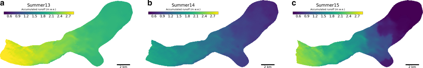
Fig. 4. Modelled SMB (upper panel) and modelled surface runoff (lower panel) at three different elevations.
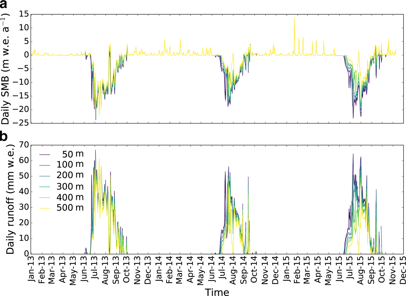
Fig. 5. Modelled accumulated surface runoff (in m w.e.) for summers (a) 2013, (b) 2014, (c) 2015.
4.2. Model accuracy and sensitivity
We assess the performance of the inversion by comparing modelled and observed velocities. Figure 6a shows the Normalised RMSE (NRMSE) between modelled and observed velocities, normalised by the mean observed velocities from 11 August 2013 to 22 August 2013.

Fig. 6. NRMSE between observed and modelled velocities normalised by the mean observed velocities (a) for the surface velocity observation from 11 August 2013 to 22 August 2013 (the filtered data are removed) and (b) time averaged with the SD band as a function of surface velocity bins for points at elevations lower than 500 m a.s.l.
Figure 6b shows the time averaged (over the entire modelling period) NRMSE plotted as a function of surface velocity bins for the surface points situated at elevations <500 m a.s.l., where the velocities are the highest and the errors negligible. The NRMSE plotted for each time period is in the same order of magnitude as the average with largest variations for low velocities. The model results match the observations within 10% in most of the domain. However, it performs less well in the upper zone (higher relative measurement error with lower velocities), the tributary glacier (rather scarce data in general), along the boundary with Kongsvegen and at places with steps bedrock gradients. These patterns are constant in time with slight variation of magnitude but no seasonal trend. The patchy nature of the errors on the upper part of the domain, upstream of step 3, largely depends on the errors due to velocity acquisition, which are relatively high in this region of low velocity.
We test the sensitivity of the model in relation to three input data: the observed velocities, basal topography and surface topography. A random normally distributed noise was applied on the gridded maps (and not on measured points) given the uncertainty of each input. We performed this analysis on one setup in July 2013 with 40 different runs for each input, 20 with an optimistic scenario (error 1, e 1, with maximum error equal to the given SD uncertainty of the input) and 20 with a pessimistic scenario (error 2, e 2, with SD error of the normal distribution equal to the given SD uncertainty of the input) as shown in Figure 7. Errors generated by velocities are small in both scenarios, whereas those generated by surface and bed topographies are generally high for the pessimistic scenario. For the bed topography, the random normal distributed noise was applied on the gridded maps (and not on measured points). This explains the large sensitivity to the bed topography in the pessimistic scenario as the accuracy of the measured depth points are not propagating randomly to each gridded cell so that such a scenario is less likely. The surface topography is also determining the surface gradient, which in turn has a great influence on the ice dynamics. Adding a large amount of random noise to the elevation would also affect the gradient in an unrealistic fashion and increase output errors. Also, where the ice is the fastest, the ice thickness is generally small (around 100 m at the front) and large errors are particularly affecting the result.
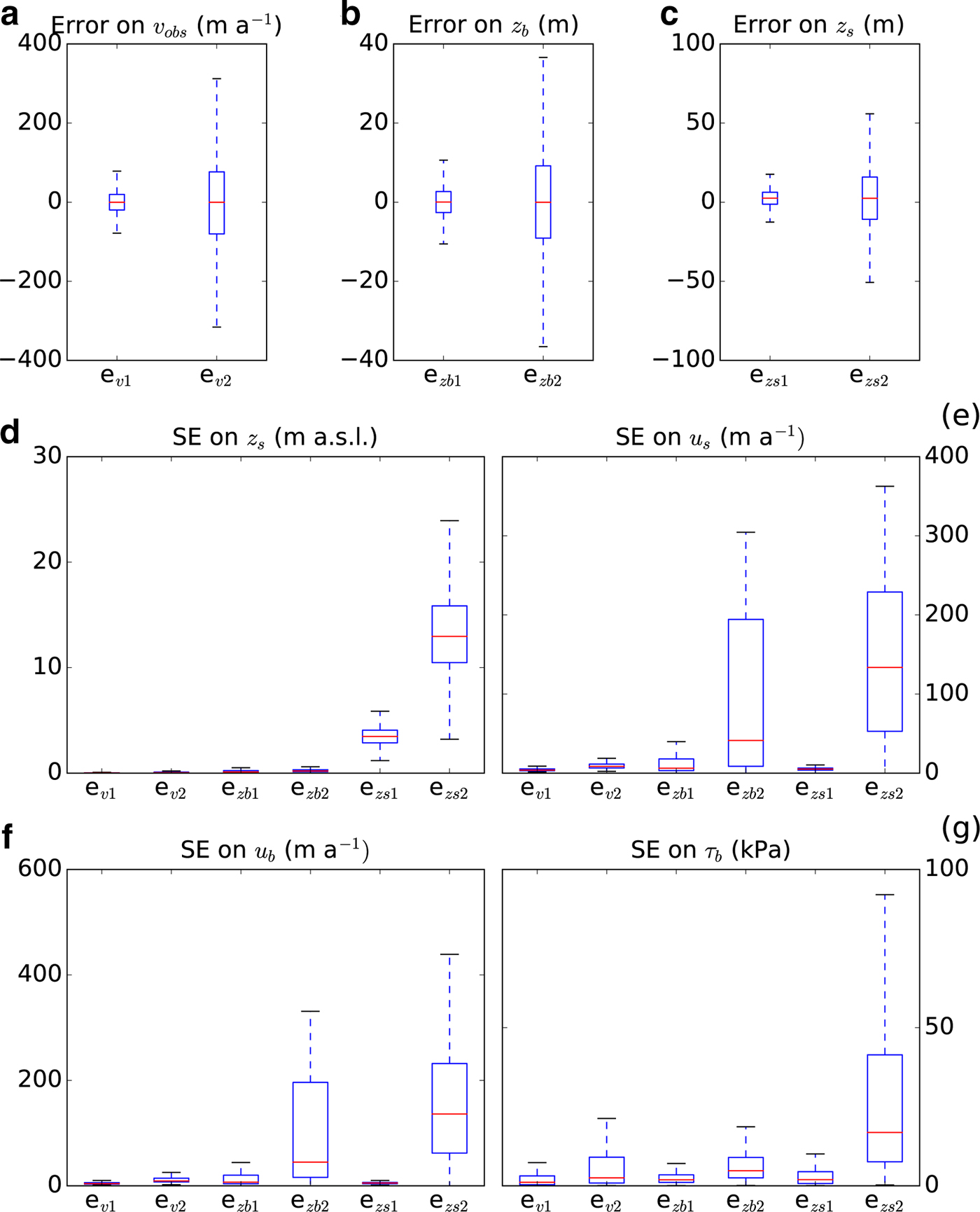
Fig. 7. Box plots of the input errors on gridded maps for two error scenarios of (a) observed surface velocity, u obs (e v1, e v2), (b) basal topography, z b (e zb1, e zb2) and (c) surface topography, z s (e zs1, e zs2) for points lower than 500 m a.s.l. elevation. SD error (SE) of (d) the surface elevation after the model run, z s, (e) the surface velocity, u s, (f) the basal velocity, u b and (g) the basal friction, τ b.
4.3. Seasonal evolution along a flow line
The inversion is performed at each acquisition time of the observed surface velocities.
For each run, basal friction coefficients, β, are optimised at the base (see Fig. 8). For visualisation purposes, we show the spatial and seasonal evolution of these quantities along a flow line (Fig. 9). Where the velocity is relatively low (<150 m a−1), the model misfit errors are too large for the results to be considered reliable (Fig. 6), so we focus on the evolution of the lower, fast-flowing tongue of Kronebreen (below 500 m a.s.l).
The crevassed area of the Kronebreen tongue ends approximately at the upper limit of the flow line. As shown at the bottom of Figure 9, we divide each year into four time periods related to their melt or calving situation. Spatial variations along the flow line are divided in six zones as shown at the left of Figures 9b, c and on Figure 8. These spatial zones and seasonal periods highlight the different patterns in the basal velocity and the topography. Three locations of surface and bed steps are particularly steep, at 5, 8 and 12 km from the front.

Fig. 8. Basal friction coefficient, β, for the surface velocity observation from 11 August 2013 to 22 August 2013. The black line represents the central flow line used to visualise the results.

Fig. 9. (a) The three upper panels (i–iii) show (i) the spatially averaged daily runoff (mm w.e.), (ii) the surface elevation during the simulation time period, z
s, anomaly to the mean (m) and (iii) the modelled surface velocities (m a−1), v
mod, averaged for each zone along the flow line. The fourth upper panel (iv) shows the frontal ablation rate, ${\dot a}_w$
, (Gt a−1). Pseudocolour plot of (b) basal tangential velocity, u
b, (c)basal shear stress, τ
b in a logarithmic scale along a flow line in distance from the most extended front position (km) and time for 2013–15. The flow line is divided in six zones and the year in four seasons (winter W, spring Sp, summer S, autumn A). The right panels of (b, c) show the topography along the flow line (bed in black and surface of the longest front in dashed black).
${\dot a}_w$
, (Gt a−1). Pseudocolour plot of (b) basal tangential velocity, u
b, (c)basal shear stress, τ
b in a logarithmic scale along a flow line in distance from the most extended front position (km) and time for 2013–15. The flow line is divided in six zones and the year in four seasons (winter W, spring Sp, summer S, autumn A). The right panels of (b, c) show the topography along the flow line (bed in black and surface of the longest front in dashed black).
During the 3 years of observations, the calving front retreated ~1.2 km and the glacier area was reduced by ~ 2.6 km2. The glacier underwent overall surface lowering through the study period, except steps 1 and 2, and a region downstream of step 3 (zone 5), where the thickness increased until spring 2014 and decreased from summer 2014. The thinning was particularly pronounced not only at the front of the glacier, but also at the foot of step 3 (uppermost part of zone 5), at the bed elevation z b = 0 m a.s.l.
4.4. Spatio-temporal variability
4.4.1. Variation with velocity
Comparing glacier-wide mean basal tangential velocities and basal shear stresses (Figs 10a, b) shows that different parts of the glacier exhibit contrasting velocity--stress relationships. In zones 5 and 6, where the velocity is almost everywhere <300 m a−1, there is an inverse relationship between velocity and stress, which varies from 20 to 200 kPa. τ b/τ d (Figs 10c, d) is typically >0.6, and numerous points where the ratio exceeds 1 denote areas of the bed that support some non-local stresses in addition to the local driving stress. In contrast, in zone 1 there is consistently low basal shear stress (<20 kPa) and a wide range of velocities from 600 to 1600 m a−1. Basal shear stress in zone 2, spread from 10 to 40 kPa, is particularly sensitive to the season, and is distributed over a smaller range of velocities (300–1000 m a−1). The ratio τ b/τ d, in zones 1 and 2, is consistently <0.5 and generally ~ 0.3, exhibiting no unique relationship with velocity. This indicates that low-strength regions of the bed that support <30% of the driving stress play little role in controlling the speed of the glacier. In these areas, most of the driving stress is supported non-locally by regions of high bed strength, such as regions close to the northernmost margin or with higher bed elevation such as bed bumps (see Fig. 3), implying that the glacier is effectively decoupled from the bed. Data from zones 3 and 4 form a cloud of points with no obvious trend, indicating highly variable behaviour of the basal shear stress and yet fairly low support of the driving stress.

Fig. 10. (a, b) Basal shear stress, τ b and (c, d) ratio of the basal shear stress over the driving stress (negative with reverse surface slope) averaged over each zone for each run along the flow line as a function of the velocity. Markers represent the six zones and colours represent the seasons (summer seasons are indicated by thicker surrounded black lines). The SDs are shown in dashed lines. Light grey dots show all points below 500 m a.s.l. elevation. (b, d) plots two zones at a time.
4.4.2. Basal friction variation over time
Between the different seasons, β m , the temporally averaged spatial pattern of β, shows different behaviours of glacier flow as shown in Figure 11. The spatial pattern of winter, spring and summer 2013 are similar and show a relatively well-distributed sliding in the first few kilometres from the front and slightly higher at the lee of steps 1 and 2. In autumn 2013, winter 2014 and spring 2014, the sliding is mostly concentrated at the front. From summer 2014 to winter 2015, sliding is high at the front and at the lee of steps 1 and 2.
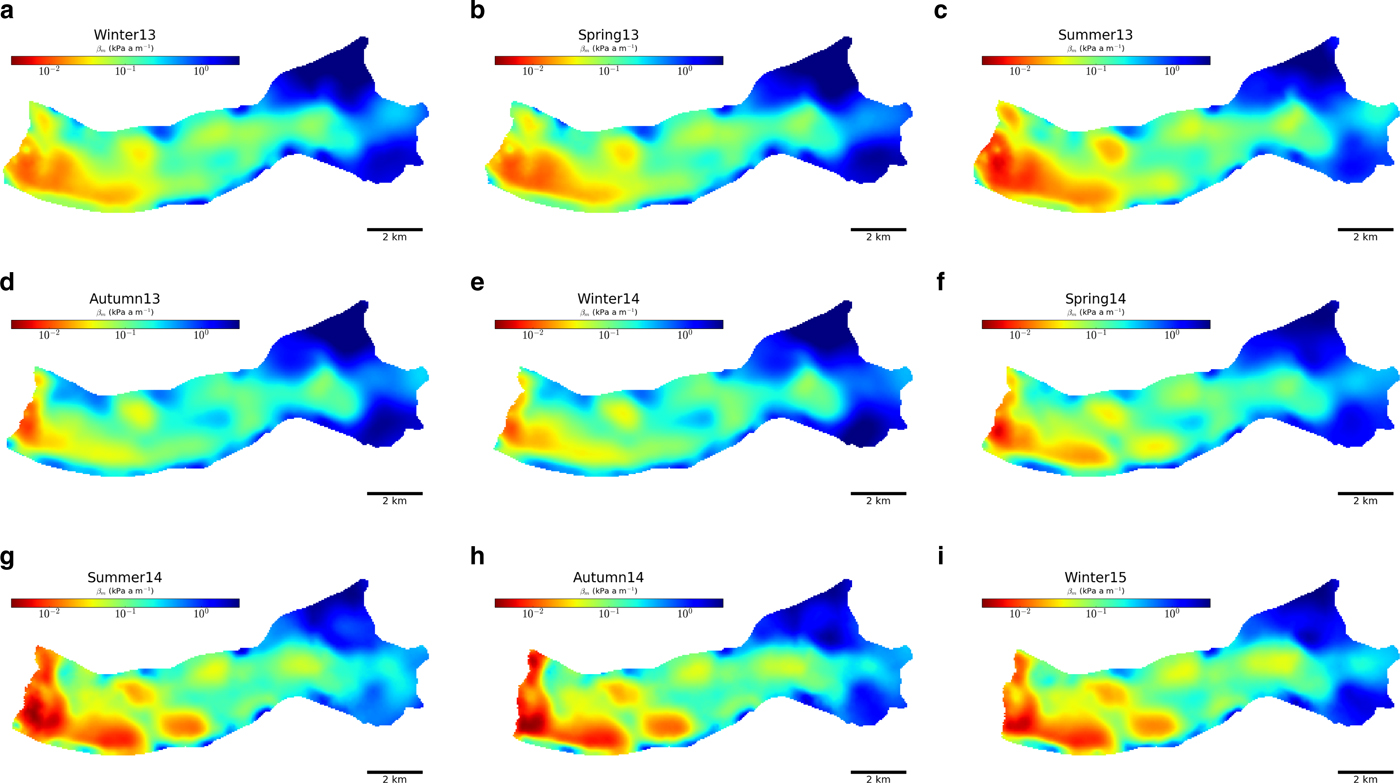
Fig. 11. Seasonally averaged basal frction coefficient β m map for points lower than 500 m a.s.l. elevation.
The year 2013 exhibits more spatial than temporal variation outside the summer (melt season). The magnitude of variability differs between the zones but changes little over time especially during winter-spring 2013. It reverts to similar values after the summer suggesting that the spatial variability is conditioned by inherent properties of the bed outside the melt season (such as bed topography, roughness and sediment distribution). By contrast, summer 2013, has a high temporal variability (coefficient of variation, defined as the ratio of the SD and the mean of the variable, CV~ 40–65% depending on the zone), although the spatial variability remains more or less similar. This suggests that the subglacial hydrology was probably changing in time though consistently over a large area confirming that temporal variability in bed friction is connected to the evolution of subglacial hydrology. A different pattern of variability in basal properties is demonstrated in 2014. Temporal variations during summer 2014 are not as large as summer 2013 (CV~ 25–45%) but with more spatial variations (CV~ 15–70%). Changes in spring 2014 at step 1 (zone 2) and step 3 (zone 6) are particularly responsible for this high spatial variation.
4.4.3. Forward modelling with averaged basal friction coefficient
Here we test the feasibility of using a temporally fixed parameterisation of the basal friction. We simulate years 2013/14 with a linear sliding law using the mean basal coefficient maps from summer 2013 (β m S 13), summer 2014 (β m S 14), both having different spatial patterns (Figs 11c, g) and from the whole time period (β m All seasons). Figure 12 shows that the forward simulation with seasonally averaged basal friction coefficients performs generally better outside of the melt season and particularly during the year of the averaged season. The forward modelling with basal friction coefficients averaged over the whole period performs better than the seasonal average outside of the melt seasons but is worst during the melt seasons. The variable character of the melt season in terms of sliding is not reproducible with an averaged basal friction parameter and leads to greater discrepancy. Overall, the forward simulation does not perform well and the RMSE between observed and modelled velocities is not constant from one year to another during the same season.
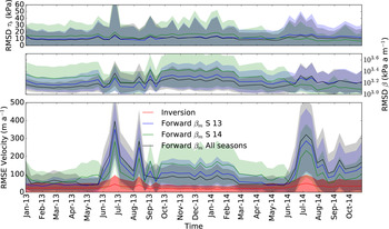
Fig. 12. Simulation with temporally averaged basal friction coefficient of summer 13, β m S 13, and summer 14, β m S 14. (a) shows the root mean square deviation (RMSD) in τ b, (b) shows the RMSD in β and (c) the RMSE between modelled and observed velocities for points below 500 m a.s.l. elevation.
4.4.4. Weertman friction law
In order to test the non-linearity of the basal sliding, we try to fit the most commonly used Weertman sliding law (Weertman, Reference Weertman1957) of the form
 $$ \tau_{\rm b} = \lpar Cu_{\rm b}^{\lpar 1 / m \rpar -1}\rpar u_{\rm b}\comma $$
with m = [1, 3, 5, 10, 15, 20, 100], the stress exponent and C > 0, a scalar assumed independent of u b and τ b. The construction of this law is based on regelation and viscous creep on a hard bed and m is usually equal to n = 3, i.e., the creep exponent of the Glen's flow law. However, if m < n, Hindmarsh (Reference Hindmarsh1997) suggested Eqn (7) can be representative of viscous deformation of the subglacial till at large scales. If m ≫ n, on the contrary, Eqn (7) represents plastic till rheology (Tulaczyk, Reference Tulaczyk2006) or ice flowing over a rigid bed with cavities (Schoof, Reference Schoof2005).
Fitting the Weertman-type law for all points at all time (Fig. 10a) would mean that all points have a similar stress exponent, m, and C at all times. The rate weakening shape of the curve does not allow such a law unless the stress exponent is negative. For each season, the stress exponent m > 0 that best fit Eqn (7) varies greatly with time (black line in Fig. 13). For each zone (coloured lines in Fig. 13), there is not a noteworthy pattern of stress exponent that stands out.
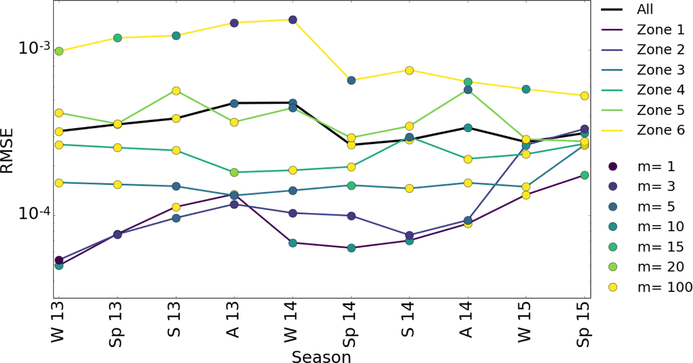
Fig. 13. RMSE for the best m in Eqn (7) per season for all points and per zone.
Equation (7) has also been fitted at each point for all dates and for each season as shown in Figure 14. Fitted over all seasons, the pattern of best m is not spatially homogeneous and values are generally very high, possibly suggesting a plastic deformation of the till. The coefficient of determination is R 2 = 0.69. Fitted for each season, the pattern is still inhomogeneous in space but also very different in time. However, coefficients of determination are higher than R 2 = 0.9 in winters and springs and closer to R 2 = 0.8 for summers and autumns. The coefficient of determination is R 2 = 0.79, R 2 = 0.76, R 2 = 0.67 and R 2 = 0.72 when fitted over the three winters, springs, summers and autumns, respectively. Once again, a single spatio-temporal value of m is not adequate. Moreover, if allowed to be negative, regions with high stress exponents appear to be even better fitted with a negative m.

Fig. 14. Best fitted m from Eqn (7) (a) at each point below 500 m a.s.l. for all dates (flow line indicated in black), (b) along the flow line for all dates (left panel) and for each season (right panel).
5. DISCUSSION
5.1. Influence of the surface runoff on the basal properties
During the two melt seasons covered by the velocity observations, the glacier exhibits a variety of dynamical patterns in ice motion (see Fig. 9). Some of the differences between the years can be explained by variations of surface runoff between the years.
The melt season in summer 2013 started slightly earlier and ended later than summer 2014 with larger mean daily runoff (~19 mm w.e. compared with ~11 mm w.e.). Moreover, the spatial extent of surface runoff was greater for summer 2013 than for summer 2014, indicating that more water was produced at higher elevations. Surface velocities in summer 2013 show a generally good correlation with surface runoff (see Fig. 9a), with three velocity peaks of diminishing intensity, but with some significant differences in detail suggesting the drainage system was adjusting through time. The first velocity peak coincided with rapidly rising runoff, but the velocity then decreased despite continuing high runoff. This suggests a switch from inefficient to efficient subglacial drainage (Hooke and others, Reference Hooke, Calla, Holmlund, Nilsson and Stroeven1989; Hubbard and others, Reference Hubbard, Sharp, Willis, Nielsen and Smart1995; Fountain and Walder, Reference Fountain and Walder1998; Shepherd and others, Reference Shepherd2009; Sole and others, Reference Sole2011; Moon and others, Reference Moon2014). The second velocity peak, in August 2013, occurred after a sharp drop in runoff that was immediately followed by a high peak. This suggests that the efficient drainage system started to close down and was unable to discharge the renewed influx of water from the surface. A third velocity peak followed a similar pattern, although lower in magnitude. The basal friction, which was relatively stable before summer 2013, reflects the variations in velocity and surface runoff during the summer, supporting the conclusion that surface-to-bed drainage was the dominant control on glacier dynamics. The slightly lower velocity and higher basal friction after the summer compared with previous winter suggests that the drainage was sufficiently efficient to evacuate much of the basal water. According to Schellenberger and others (Reference Schellenberger, Dunse, Kääb, Kohler and Reijmer2015), summer 2013 was the most extensive speedup of the period 2010–13.
In summer 2014, the ice front geometry was more variable, the melt season was shorter in duration and less water was produced at the surface. Changes in velocity and the basal friction coefficient show some relationship with surface runoff, but there are important differences compared with summer 2013. A first velocity peak at the beginning of July, coincides with a water runoff peak, mostly produced in zone 1, and the onset of ice front retreat likely associated with the decrease in backstress. Despite the fact that meltwater input was confined to the terminus region, the increase in velocity took place far up-glacier. A second peak in velocity at the beginning of August, affecting only zones 1 and 2, occurred while surface runoff was low, but during a peak in calving losses. A third velocity peak at the beginning of September, also mainly affecting zones 1 and 2, coincided with a late-season peak in runoff. However, velocities in zones 1 and 2 remained high at times of low runoff, suggesting that an efficient drainage system did not fully develop, encouraging high basal water pressures, or that the front became unstable because of calving.
Some changes in the basal friction also appear to be related to changes in surface topography. For example, the gradual reduction in τ b in zone 5 (below surface step 3) began in spring 2014, probably caused by ice thickness reduction in this zone that had undergone previous thickening. The basal friction in this zone continued to decrease until summer 2015, which contrasts the increases in all other zones following summer 2014. The velocity evolution during 2014 could also have been influenced by the rapid retreat of the front due to loss of backstress induced by increased calving (Fig 9a).
This analysis is in line with the conclusions of Moon and others (Reference Moon2014) that glacier behaviours in Greenland reflect the relative impacts of surface runoff and calving front retreat. Sundal and others (Reference Sundal2011) also noticed that surface peak rates of ice speed-up were correlated to surface runoff but not mean summer flow rates for some glaciers in Greenland. At the interannual timescale, Sole and others (Reference Sole2013) and Tedstone and others (Reference Tedstone2015) suggested that summer runoff was strongly correlated with autumn–winter ice motion rather than annual ice flow. The time span of our observations is unfortunately too short to draw any general conclusion, but it is clear from the results that late summer ice dynamics influence autumn and winter velocities.
5.2. Variability and sliding behaviour
The spatial and temporal variability of basal friction can be a consequence of two types of control. The spatial pattern, which does not significantly change over time, reflects constant properties of the bed such as the bed roughness or bed gradient. Changes in spatial variability over time or in temporal variability, in general, are indicative of variations in external forcing such as ice thickness, surface runoff, stress gradients and modifications to the subglacial hydrology. The fact that the spatial and temporal patterns of basal friction are so different between the years indicates how problematic the use of a spatio-temporally constant basal friction coefficient or a simple sliding law is when trying to simulate short timescale (seasonal) velocity variations.
It is evident from the forward modelling presented in Figure 12 that a spatially variable but temporally fixed basal friction coefficient for a linear sliding law fails to reproduce the sliding behaviour of Kronebreen over time. Errors become larger outside of the season the parameter was optimised for and during periods of high variability such as the melt seasons. Likewise, a non-linear sliding law of Weertman-type with single friction and stress coefficients does not show a good fit for all points at all time steps (Fig. 13). When fitted at each point (Fig. 14), over spatial zones and seasons, the values of m differ greatly and preclude a uniform value. Isolated from the rest of the year, the fit for each season, apart from the melt season, is relatively good (same spatially variable C and m in Eqn (7)), but fails when the same parameters are used either for a similar season or for the whole period. In any case, high values of m in most of the domain show that the Weertman sliding law fails to model the reality properly. Furthermore, the velocity weakening tendency (best fit for m < 0) reveals a particular behaviour of the bed. This decreasing basal resistance with increasing slip velocity, called the velocity or rate weakening (Scholz, Reference Scholz2002), is discussed theoretically by Schoof (Reference Schoof2005) and exerimentally by Zoet and Iverson (Reference Zoet and Iverson2016) in the case of hard beds where cavities can grow in the lee of bumps. In the case of soft beds, a laboratory study by Thomason and Iverson (Reference Thomason and Iverson2008) assessed the role of particle ploughing and pore-pressure feedback in velocity weakening mechanism that have been observed (e.g. Rousselot and Fischer, Reference Rousselot and Fischer2005). Unfortunately, no existing measurement or direct evidence can help to constrain any of these theories.
The variability of m could represent a variety of processes such as viscous or plastic deformation but can also arise from different bed properties, seasonal changes in surface elevation or in subglacial drainage. As discussed above, surface runoff or thickness changes, influencing effective pressure variations in turn, must play an important role in spatio-temporal changes not only locally but also non-locally, as suggested by the persistent high velocities after the melt season in 2014.
The patterns in Figure 10 suggest the sliding behaviour reflects contrasting effects. On the upper part of the glacier tongue, in zones 5 and 6, where the bed generally supports most of the driving stress and other non-local stresses in some cases, a local sliding law could provide a valid means of characterising the inverse relationship between u b and bed strength. However, on the lower tongue where the bed is not supporting the driving stresses, a ‘local’ friction law (meaning that velocities are uniquely associated with particular basal stresses) would fail to capture the important role that ‘non-local’ sources have in controlling rates of glacier flow. The range of variation in u b for zones 1 and 2 is associated with almost constant values of τ b.
Over the 3 years of observation, the inversion of the surface velocities gives an insight into the basal properties and their evolution. We observe the wholesale changes in areas of the bed that are capable of supporting the local driving stress and little change in areas that do not. In general, it seems that in some situations there is a progressive reduction over time in the area of the bed resisting the driving stress, presumably as a consequence of a reduction in local effective pressure. The implication is that an increasing part of the glacier area is progressively supported by a steadily shrinking area of the bed, i.e., the area of the bed with minimal basal drag is likely to increase in the future so that at the glacier scale, lateral support becomes more critical. The weakly grounded downstream areas that do not fully support the driving stress and are subject to loss of buttressing at the front, transfer stresses longitudinally upstream to the stronger areas seasonally modulated by the downstream areas speedup. Some of this acceleration could be due in turn to seasonal weakening of the upstream area. Weak beds can be covered by a continuous till layer and experience low effective pressures. If this is the case, and in addition to a plastic bed behaviour, the till can be in a constant critical state (Hindmarsh, Reference Hindmarsh1997) with small, localised slip events more common than glacier-wide slip-events and globally controlled.
This study is done on a relatively short timescale focusing on the seasonal/interannual variations in response to a change in water at the ice sheet bed. It is thus impossible to draw any firm conclusion on the role of these variations on the longer-term behaviour and which trends are the most important.
6. CONCLUSION AND OUTLOOK
This study shows the spatial and temporal variations of basal motion for a fast-moving outlet glacier in Svalbard on the seasonal/interannual timescale. These variations appear primarily driven by the amount of meltwater reaching the bed and its influence on the subglacial hydrological drainage system. When these changes to the basal environment are in concert with surface runoff and front retreat, two different patterns are evident. The first summer (2013) is mostly influenced by the basal properties evolving alongside the development of the subglacial drainage system fed by water routed to the bed. This water is sufficiently well evacuated for velocities to return to background values at the end of the season. During the second summer (2014), the glacier, experiencing important geometric changes, appears to be unable to accommodate the water and maintains high velocities during the following winter.
The basal friction coefficient, linking the basal velocity to the basal shear stress, exhibits substantial spatio-temporal variation, precluding the use of a temporally fixed Weertman-type sliding law or at least not on the whole domain. The corollary is that sliding laws used in prognostic models need to be capable of capturing these temporal variations in friction if they are to model ice velocities accurately. In particular, models need to be able to capture the local and non-local influences on bed resistance in time and space, such as those generated by changes in basal hydraulics. This effect is usually included in sliding laws through the effective pressure but is poorly implemented in real cases because water pressures are difficult to constrain.
Prognostic simulations for glaciers, such as Kronebreen, influenced by seasonal water production, will need not only to incorporate a suitably spatio-temporal adaptive sliding law, but also predict the calving behaviour to reproduce the loss of buttressing. Additional ongoing work on basal hydrological modelling using the Werder and others (Reference Werder, Hewitt, Schoof and Flowers2013) model may help to elucidate the influence of water on sliding during and after the melt season, and to determinate the spatio-temporal validity of different sliding laws such as a simple Weertman-type or a more complex effective pressure based law.
ACKNOWLEDGMENTS
This project was financially supported by the Greenland Analogue Project (GAP) and the Nordic Centre of Excellence SVALI. Acquisition of the TerraSAR-X imagery was funded by the ConocoPhillips Northern Area Program, via the CRIOS project (Calving Rates and Impact on Sea Level). The leading author received an Arctic Field Grant from the Svalbard Science Forum to acquire radar lines for the basal topography in 2014. We thank CSC -- IT Center for Science Ltd. for the CPU time that was provided under the Nordic Center of Excellence SVALI (Stability and Variations of Arctic Land Ice). Thomas Zwinger was supported by the Nordic Center of Excellence eSTICC (eScience Tools for Investigating Climate Change in Northern High Latitudes) funded by Nordforsk (grant 57001). We thank Fabien Gillet-Chaulet and Olivier Gagliardini for their insights on inversion, sliding and Elmer/ICE. The authors are grateful to DLR for the provision of TanDEM-X IDEM data (project GLAC0213).


 Open access