


1. Introduction
A jet in cross-flow (JICF) consists of a jet of fluid with mean velocity  $\bar {U}_{{jet}}$ exiting perpendicularly to a cross-flow of velocity $U_{\infty }$. JICFs are relevant to a variety of engineering applications, such as fuel injectors, turbine blade cooling and dilution jets in combustors, and therefore have been the focus of considerable research interest. Much of the past work on JICFs is summarized in reviews by Karagozian (Reference Karagozian2010) and Mahesh (Reference Mahesh2013). An incompressible JICF with matched jet and cross-flow density ( $\rho$) and kinematic viscosity ( $\nu$) can be characterized by the jet Reynolds number, $Re_j = \bar {U}_{{jet}} D/\nu$, and the jet-to-cross-flow velocity ratio, $R = \bar {U}_{{jet}}/U_{\infty }$, where $D$ is the jet exit diameter, $\bar {U}_{{jet}}$ is the mean velocity of the jet at the jet exit and $U_{\infty }$ is the free-stream velocity of the cross-flow. Alternatively, a JICF may be described by the momentum flux ratio $J = \rho _{{jet}} \bar {U}_{{jet}} / \rho _{\infty } U_{\infty }$ to incorporate differing jet ( $\rho _{{jet}}$) and cross-flow ( $\rho _{\infty }$) densities.
Despite the relatively simple boundary conditions, the flow field of a JICF is made up of the complicated interaction of several vortical structures. At low velocity ratios (nominally less than 1), hairpin vortices dominate the interaction between the jet and cross-flow (Mahesh Reference Mahesh2013). Ilak et al. (Reference Ilak, Schlatter, Bagheri and Henningson2012) found that, as  $R$ increases, the first instability of the transverse jet is through a Hopf bifurcation which produces self-sustained oscillations in the jet's downstream shear layer (DSL) to create hairpin vortices. This first application of wavemaker analysis for a three-dimensional flow was confirmed by the carefully detailed experiments of Klotz, Gumowski & Wesfreid (Reference Klotz, Gumowski and Wesfreid2019), and Chauvat et al. (Reference Chauvat, Peplinski, Henningson and Hanifi2020) found that in this regime the jet was very sensitive to small perturbations below absolutely unstable values of $R$.
$R$.
For the remainder of the paper, we will focus on jet velocity ratios above unity, where the flow structures of the JICF are markedly different. The most recognizable feature of a JICF in this regime is the counter-rotating vortex pair (CVP) that has been shown to dominate the jet cross-section far downstream of the jet exit (Kamotani & Greber Reference Kamotani and Greber1972; Smith & Mungal Reference Smith and Mungal1998), although the instability of the upstream shear layer (USL) has also been of great interest. For jets with flush exit orifices, a horseshoe vortex system forms in front of the jet. While these vortices bear some qualitative similarities with horseshoe vortices formed in front of solid obstacles, horseshoe vortices of JICFs show some differences including differing modes based on  $R$ (Kelso & Smits Reference Kelso and Smits1995). Kelso, Lim & Perry (Reference Kelso, Lim and Perry1996) suggested that, depending on the sign of their vorticity, horseshoe vortices can be lifted and absorbed into the CVP. Additionally, upright wake vortices extending vertically from the wall to the jet have been observed in the wake and attributed to separation events in the cross-flow boundary layer due to the adverse pressure gradient imposed by the jet entrainment (Fric & Roshko Reference Fric and Roshko1994; Schlegel et al. Reference Schlegel, Wee, Marzouk and Ghoniem2011).
The stability of JICFs has also been the subject of several studies. Megerian et al. (Reference Megerian, Davitian, Alves and Karagozian2007) and Davitian et al. (Reference Davitian, Getsinger, Hendrickson and Karagozian2010) experimentally studied a JICF at fixed Reynolds numbers of 2000 and 3000 over a range of  $R$ values. They found that for $R > 3.2$, there was frequency shifting in the spectra moving along the USL, which was attributed to tonal interference of the probe and the instability frequency (Hussain & Zaman Reference Hussain and Zaman1978). These findings indicated characteristics of a convectively unstable shear layer, where disturbances are amplified downstream of their initiation (Huerre & Monkewitz Reference Huerre and Monkewitz1985). Decreasing $R$ while maintaining a fixed $Re_j$ led the USL instabilities to become stronger, increase in frequency, and move closer to the jet exit. For $R < 3.2$, Megerian et al. (Reference Megerian, Davitian, Alves and Karagozian2007) observed single frequency instabilities in the USL with strong harmonics that formed almost immediately after the jet orifice, indicative of an absolute instability, where the flow becomes self-excited (Huerre & Monkewitz Reference Huerre and Monkewitz1990). Bagheri et al. (Reference Bagheri, Schlatter, Schmid and Henningson2009) performed linear stability analysis of a JICF at $R = 3$ using a base flow obtained by selective frequency damping. They showed that the jet was characterized by self-sustained global oscillations, and that unstable high-frequency global eigenmodes were associated with the USL, while low-frequency modes were associated with the wake of the jet inside the boundary layer. Iyer & Mahesh (Reference Iyer and Mahesh2016) studied the USL of a JICF at $Re_j = 2000$ and $R = 2$ and 4, discovering an analogy between the jet upstream mixing layer and a counter-current mixing layer could be used to explain the convective and absolute instability regimes of the USL. This counter-current shear layer analogy was extended by Shoji et al. (Reference Shoji, Harris, Besnard, Schein and Karagozian2020) to a range of jet momentum flux ratios and density ratios at several values of $Re_j$ using an extensive set of experiments.
Regan & Mahesh (Reference Regan and Mahesh2017) performed global linear stability analysis based on the time-averaged mean flows considered by Iyer & Mahesh (Reference Iyer and Mahesh2016). The choice to use the turbulent mean flow as the base state was motivated by a scale-separation argument to justify that the Reynolds stress terms for the modes of interest were negligible. Note that stability analysis using time-averaged mean flow has been found to underpredict growth rates, but correctly predict instability frequencies (Bagheri et al. Reference Bagheri, Schlatter, Schmid and Henningson2009; Ma & Mahesh Reference Ma and Mahesh2022). Regan & Mahesh (Reference Regan and Mahesh2017) were able to produce Strouhal numbers which matched the direct numerical simulation (DNS) spectra and dynamic mode decomposition (DMD) of Iyer & Mahesh (Reference Iyer and Mahesh2016) and the experiments of Megerian et al. (Reference Megerian, Davitian, Alves and Karagozian2007). They also provided evidence for the shift from absolute to convective instability of the USL as  $R$ is increased from 2 to 4, and point out that the location of the most unstable eigenvalue is in the DSL for $R = 4$. This points to the DSL's significance at higher $R$. Regan & Mahesh (Reference Regan and Mahesh2019) applied adjoint sensitivity and optimal perturbation analysis to the same jet configuration, finding that the jet at $R = 4$ showed a DSL instability with a higher growth rate than the USL, as well as higher growth rates for asymmetric instabilities than the jet at $R = 2$. This explained asymmetric CVP states that were observed in experiments at higher $R$ (Smith & Mungal Reference Smith and Mungal1998; Getsinger et al. Reference Getsinger, Gevorkyan, Smith and Karagozian2014). The adjoint modes and optimal perturbation analysis of Regan & Mahesh (Reference Regan and Mahesh2019) also pointed to the most sensitive regions for forcing. The upstream shear layer modes for both $R = 2$ and $4$ were most sensitive to regions at the upstream edge of the nozzle exit, while asymmetric modes were most receptive to actuation at either side of the upstream edge of the jet exit.
There has been considerable interest in finding ways to control jet trajectories and mixing using passive devices. The study of tabs affixed to the exit of regular jets (where  $R \rightarrow \infty$ such that there is zero cross-flow) stretches back to the work of Bradbury & Khadem (Reference Bradbury and Khadem1975), who found that the insertion of small tabs produced large effects on the jet cross-section and enhanced entrainment. They attributed these effects to the deflection of the flow around the tab rather than vortices produced by the tab, based on a simple visualization of a wool tuft affixed near the tab. Ahuja & Brown (Reference Ahuja and Brown1989) came to many of the same conclusions for tabs affixed to high-speed and heated jets, finding that tabs effectively eliminated screech noise from supersonic jets and suggesting that there must be a train of secondary structures that enhances mixing. This mixing improvement was also echoed by Zaman (Reference Zaman1996), who found that a nozzle with tabs far exceeded the mixing performance of other nozzle geometries. Zaman, Samimy & Reeder (Reference Zaman, Samimy and Reeder1991) also found that the tab induced an indentation of the shear layer that grows with downstream distance, which they attributed to streamwise vortices originating from the tips of the tab (rather than horseshoe vortices from the base of the tab). The origin of these streamwise vortices was explained via an inviscid pressure-driven phenomenon, requiring that a favourable pressure gradient is produced across the tab. A similar explanation using the vorticity transport equation was suggested by Reeder & Samimy (Reference Reeder and Samimy1996) based on measurements of a regular jet with tabs. Zaman, Reeder & Samimy (Reference Zaman, Reeder and Samimy1994) attributed the streamwise vortices to two sources: a dominant source from the ‘pressure hill’ (and associated lateral pressure gradients) generated by the tab and a secondary source due to sheets of vorticity shed by the tab and reoriented into the streamwise direction by the mean shear of the mixing layer. They explain that this secondary generation process may result in vorticity of the same sign as the primary vorticity for tabs with downstream-leaning apexes, and the opposite sign of vorticity for apex-upstream tabs. Foss & Zaman (Reference Foss and Zaman1999) found that the addition of streamwise vortices due to the tab increased the population of small-scale structures in a plane shear layer, hence leading to an increase of both large-scale and small-scale mixing. Island, Urban & Mungal (Reference Island, Urban and Mungal1998) performed a similar study, finding that three-dimensional disturbances of only 5 % of the boundary layer thickness were much more effective compared with two-dimensional disturbances at thickening and enhancing mixing of the shear layer.
The first study of tabbed JICFs was performed by Liscinsky, True & Holdeman (Reference Liscinsky, True and Holdeman1995), who conducted experiments to investigate the effects of various tab and slot configurations for a JICF at  $J = 8.5$ and $Re_j = 24\ 000$. They concluded that a downstream tab was ineffective at altering the jet cross-section compared with a jet with both upstream and downstream tabs, which decreased jet penetration and increased spreading. However, they concluded that the tab did not significantly increase mixing and was unable to generate significant vorticity compared with that generated by the cross-flow. The effect of tabs on JICFs was later studied by Zaman & Foss (Reference Zaman and Foss1997), who experimentally investigated the effect of tabs placed at the exit of a JICF for momentum-flux ratios of 21.1 and 54.4. They found that the tab had very little effect on the penetration and spreading of the jet when placed on the leeward (downstream) side, which they attributed to an insufficient ‘pressure hill’ due to the lower static pressures on this side of the jet exit. However, they note that the virtual ineffectiveness of this tab configuration suggests a deeper explanation. On the other hand, there was a significant effect from a tab placed on the windward (upstream) side of the jet, characterized by a reduction in jet penetration and CVP strength for both values of $J$, which they attributed to opposite signs of vorticity between the tab-induced vorticity and the CVP. They also note that the dramatic effects of the tab placement on the jet cross-section suggest a high sensitivity to slight asymmetries in the tab placement. Later experiments by Bunyajitradulya & Sathapornnanon (Reference Bunyajitradulya and Sathapornnanon2005) confirmed that the mean flow is most sensitive to tabs placed on the windward side of the jet compared with the leeward side for a jet velocity ratio of $R = 4$ and $Re_j = 15\ 000$. They observed that the windward tab slightly reduced penetration depth and increased spanwise spreading of the jet cross-section, suggesting that a connection between the tab placement and the development of the skewed mixing layer and hanging vortices (Yuan, Street & Ferziger Reference Yuan, Street and Ferziger1999) could explain the relative effectiveness of different tab configurations. Zaman (Reference Zaman1998) studied the effect of tabs on transverse jet penetration for a range of $J$ from 10 to 90, finding reductions in jet penetration of up to 40 %, with greater effectiveness at higher $J$. They also found that the lateral spreading of the jet was increased for the apex-downstream tab, but reduced for other orientations of the tab.
Recently, Harris, Besnard & Karagozian (Reference Harris, Besnard and Karagozian2021) experimentally investigated the effect of triangular tabs at varying azimuthal locations for jet Reynolds numbers of 1900 and 2300. They found that tab locations with the greatest impact matched the regions most sensitive to forcing predicted by Regan & Mahesh (Reference Regan and Mahesh2019) at similar  $Re_j$. In particular, the upstream tab was most effective at promoting mixing and was observed to weaken the USL instability, aligning with the sensitivity of USL modes to perturbations at the upstream edge of the jet exit. The downstream tab also weakened the USL instability, but was completely ineffective at increasing mixing at low $R$ and only showed slight mixing improvements at higher $R$. While the upstream tab weakened the USL instability for both absolutely unstable (AU) and convectively unstable (CU) jet velocity ratios (where the labels AU and CU refer to the state of the USL), the greatest effect was observed for the naturally AU jet at lower $R$, where the upstream tab caused a switch from AU to CU behaviour. Despite this effect on the USL, tabs had a relatively small effect on the overall jet structure for the naturally AU jet, causing flattening or small asymmetries in the jet cross-section for asymmetric tab placements. In contrast, at higher $R$ (corresponding to the naturally CU USL), both the upstream and downstream tabs improved mixing, and the asymmetry of the jet cross-section could be altered through asymmetric placement of the tab, aligning with the increased growth rates of asymmetric modes for $R = 4$ predicted by Regan & Mahesh (Reference Regan and Mahesh2019) and the sensitivity of these modes to actuation on either side of the upstream edge of the jet exit. Harris et al. (Reference Harris, Besnard and Karagozian2021) suggested that the contrast in USL spectral characteristics and the jet cross-section effects ‘might imply greater changes than those actually observed in the jet structure’.
The findings of Harris et al. (Reference Harris, Besnard and Karagozian2021) and the persisting question of the specific changes to the flow field due to the tab motivate the present work. We seek to expand upon the past studies of Iyer & Mahesh (Reference Iyer and Mahesh2016) and Harris et al. (Reference Harris, Besnard and Karagozian2021) by performing DNSs of a JICF with the tab geometry of Harris et al. (Reference Harris, Besnard and Karagozian2021) at the same jet Reynolds number ( $Re_j = 2000$) and velocity ratios ( $R = 2$ and 4) studied by Iyer & Mahesh (Reference Iyer and Mahesh2016). The purpose of the present simulations is to:
(i) reveal the three-dimensional changes that the tabs induce to the USL and cross-section;
(ii) evaluate the changes in the tab-induced flow structures with variations between upstream and 45 $^\circ$ from upstream tab positions for $R = 2$ and $4$; and
(iii) provide physical reasoning for how the tab induces these effects.


The two computational tools used to achieve these goals are overset DNS, which permits a systematic study of the tab position, and DMD to reveal the dominant frequencies associated with each jet configuration.
The paper is organized as follows. Section 2 summarizes the DNS and DMD algorithms and the pertinent computational details. Section 3 overviews the instantaneous flow on the centreplane and spectra in the USL. Sections 4 and 5 discuss the effect of the tab on the USL vortical structure for the upstream and  $45^\circ$ tab positions, respectively, while § 6 discusses the influence of the tabs on the jet's DSL. Section 7 covers DMD analysis of each jet configuration. Section 8 considers time-averaged statistics, with focus on the USL and DSL instability development, local flow in the nozzle around the tab and jet penetration and cross-section. Finally, § 9 concludes the paper.
2. Numerical details
Direct numerical simulation of the tabbed JICF is performed using an unstructured overset method, and results are analysed using DMD. An overview of the numerical method for the DNS is provided in § 2.1, followed by details of the computational domain and grid configuration in § 2.2. A description of the DMD method is given in § 2.3.
2.1. Direct numerical simulation
The present computations are performed using the overset DNS method developed by Horne & Mahesh (Reference Horne and Mahesh2019a,Reference Horne and Maheshb). The algorithm is based on the unstructured grid, finite volume method developed by Mahesh, Constantinescu & Moin (Reference Mahesh, Constantinescu and Moin2004) for simulation of the incompressible Navier–Stokes equations. This method emphasizes discrete kinetic energy conservation to ensure robustness at high Reynolds numbers without added numerical dissipation, and has been validated for a variety of complex flows, including free jets (Babu & Mahesh Reference Babu and Mahesh2004) and transverse jets (Muppudi & Mahesh Reference Muppudi and Mahesh2005; Muppidi & Mahesh Reference Muppidi and Mahesh2007; Muppudi & Mahesh Reference Muppudi and Mahesh2008; Sau & Mahesh Reference Sau and Mahesh2010; Iyer & Mahesh Reference Iyer and Mahesh2016). Horne & Mahesh (Reference Horne and Mahesh2019b) extended the method to allow for overset simulation of arbitrarily overlapping and moving meshes. In an overset method, the simulation domain is made up of several overlapping body-fitted meshes, which may be free to move in six-degrees-of-freedom (6DOF) motion. Redundant cells near the boundaries of overlapping meshes are removed, exposing cell faces which require interpolated boundary conditions. The incompressible Navier–Stokes equations are written in an arbitrary Lagrangian-Eulerian (ALE) formulation as
 $$\begin{gather} \frac{\partial u_i}{\partial t} + \frac{\partial}{\partial x_j} ( u_i u_j - u_i V_j ) ={-} \frac{\partial p}{\partial x_i} + \nu \frac{\partial^2 u_i}{\partial x_j \partial x_j}, \end{gather}$$
 $$\begin{gather}\frac{\partial u_i}{\partial x_i} = 0, \end{gather}$$
where  $u_i$ are the Cartesian velocity components, $p$ is the pressure and $\nu$ is the kinematic viscosity. The mesh velocity, $V_j$, is included in the ALE formulation to avoid tracking multiple reference frames for each mesh, but this term is zero for the present case since there is no mesh motion. The overset method provides several advantages, including simplification of the grid generation process for complex geometries, computational cost savings for high- $Re$ or 6DOF flows and the ability to simulate flow about moving bodies. Issues typical of overset methods are the scaling of the method to large computations and the conservation and interpolation errors at the edges of meshes of differing levels of refinement. The first issue was addressed by the novel parallel communication structure of Horne & Mahesh (Reference Horne and Mahesh2019a) and the second by the interpolation scheme of Horne & Mahesh (Reference Horne and Mahesh2019b). This overset method has been validated for a variety of flows (Horne & Mahesh Reference Horne and Mahesh2019b) and has been applied to successfully perform large-eddy simulation of the turbulent boundary layer over an axisymmetric hull (Morse & Mahesh Reference Morse and Mahesh2021) and a ducted propulsor in crashback (Kroll & Mahesh Reference Kroll and Mahesh2022), as well as DNS of a variety of resolved particle-laden flows (Horne & Mahesh Reference Horne and Mahesh2019b).
The solution is advanced in time using a implicit Crank–Nicolson time stepping with a predictor–corrector scheme, where the velocities are predicted using the momentum equation and subsequently corrected using the pressure Poisson equation to satisfy continuity. Details of the method can be found in Horne & Mahesh (Reference Horne and Mahesh2019b).
2.2. Details of the geometry, grid and computational domain
The flow configuration for the present study consists of a circular jet centred about the origin with a laminar boundary layer cross-flow. A schematic of the problem setup is shown in figure 1, where the origin is selected to be the centre of the jet at the jet exit plane. The  $y$ axis points vertically along the nozzle centreline, while the $x$ axis is aligned with the cross-flow direction. The $z$ axis points in the spanwise direction to complete the right-handed coordinate system. The geometry of the nozzle and computational domain sizings are based on those described by Iyer & Mahesh (Reference Iyer and Mahesh2016), who modelled the nozzle shape as a fifth-order polynomial to match the experiments of Megerian et al. (Reference Megerian, Davitian, Alves and Karagozian2007). Jet velocity ratios of $R = 2$ and 4 are chosen with a constant jet Reynolds number of $Re_j = 2000$. In these definitions, $\bar {U}_{{jet}}$ is the mean velocity of the jet assuming a circular exit (ignoring the blockage of the tab). Note that the actual velocity ratios considering the tab blockage are approximately 2.048 and 4.095 for the $R=2$ and $R=4$ cases, respectively.

Figure 1. Computational domain for simulation of the JICF (taken from Regan & Mahesh Reference Regan and Mahesh2019).
The tab in the present computations is a triangular tab with a right-angled apex, matching the dimensions of the tab used in the experiments of Harris et al. (Reference Harris, Besnard and Karagozian2021). A drawing of the jet orifice cross-section with the tab dimensions labelled is shown in figure 2(b). The thickness of the tab is  $0.2012D$ and the base width of the tab is $0.25D$, resulting in a 2.3 % geometric blockage of the original circular jet. Note that in the experiments of Harris et al. (Reference Harris, Besnard and Karagozian2021), the nozzle length is extended by $0.19D$ to accommodate the tab template, which slightly weakened the shear layer compared with the original nozzle. We do not incorporate the same extension into the present simulations to permit direct comparisons with the non-tabbed results of Iyer & Mahesh (Reference Iyer and Mahesh2016) and Regan & Mahesh (Reference Regan and Mahesh2017, Reference Regan and Mahesh2019) for the original nozzle.
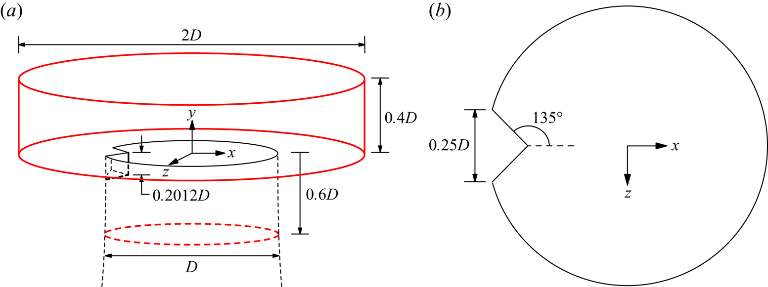
Figure 2. (a) Schematic of the tab overset grid where edges of the grid are shown in red and dimensions are provided for the overset grid boundaries and tab thickness. Panel (b) shows the top view of the upstream tab jet orifice with cross-sectional tab dimensions labelled.
In the computations, the domain is split into two grids: a background grid representing the nozzle, inflow and outflow boundary conditions, and an overset grid for the tab. The background grid does not contain the geometry of the tab and is therefore essentially a replica of the grid that Iyer & Mahesh (Reference Iyer and Mahesh2016) used to study the non-tabbed JICF, although the grid is refined near the jet orifice to interface with the tab grid. The tab grid is shaped as an inverted top-hat shape that fits into the jet exit, and contains wall boundary conditions for the tab, nozzle and cross-flow bottom wall. Figure 2(a) shows the dimensions of the tab overset grid, with the edges of the grid portrayed by red lines. A cylindrical cut is used to remove redundant cells from the background grid, with the grid overlap carefully controlled at interpolation boundaries to target matching cell sizes between the tab and background grids. A slice of the computational mesh around the jet exit and grid overlap for the upstream tab case is shown in figure 3. The split background and tab grid method greatly simplifies the grid generation process and allows the tab grid to be rotated to any angular position around the jet exit, permitting studies of various azimuthal tab locations without requiring creation of new grids. In the present work, two tab orientations are considered:
(i) Tab apex pointing in the positive
$x$-direction as pictured in figure 2 (corresponding to a tab apex vector of $1 \hat {i} + 0 \hat {k}$); and(ii) tab rotated
$45^\circ$ from upstream with the tab apex pointing in the $0.5 \hat {i} - 0.5 \hat {k}$ direction.


These configurations are termed the ‘upstream tab’ and ‘45 $^\circ$ tab’, respectively.

Figure 3. Slice of the computational mesh on the centreplane ( $z = 0$) for the upstream tab. The overlap between the background and tab grids is visible.
A uniform inflow is provided to the entrance of the jet nozzle, which is located  $13.33D$ below the jet exit, as depicted in figure 1. The cross-flow inflow boundary is located at $8D$ upstream of the origin, where a Blasius boundary layer is prescribed. The Blasius inflow profile was chosen to match the laminar boundary layer in the experiments measured with the jet off at a distance $5.5D$ upstream of the jet exit location, as in Iyer & Mahesh (Reference Iyer and Mahesh2016). The resulting momentum thicknesses at the jet exit with the jet turned off are $\theta _{{BL}}/D = 0.1215$ for the $R = 2$ configuration and 0.1718 for $R = 4$. The lateral boundaries are located a distance of $8D$ from the centre of the jet exit, while the top and outflow boundaries are $16D$ from the origin, with these boundaries being assigned zero-gradient Neumann boundary conditions.
Matching the grid sizings of Iyer & Mahesh (Reference Iyer and Mahesh2016), we maintain a spacing of  $\Delta x/D = 0.033$ and $\Delta z/D = 0.02$ downstream of the jet exit on the background grid with a minimum $y$-spacing of $\Delta y / D = 0.0013$. There are 400 points distributed around the circumference of the jet exit. The grid spacings near the jet exit are refined in all three coordinate directions compared with Iyer & Mahesh (Reference Iyer and Mahesh2016) to match the resolution of the tab overset grid, which must resolve the flow around the tab. The background grid comprises 163 million cells partitioned over 4048 processors. The tab grid comprises 16.6 million cells partitioned over 440 processors, bringing the total size of the computation to nearly 180 million cells (4488 processors). The computations are advanced implicitly in time with a non-dimensional time step of $\Delta t \bar {U}_{{jet}}/D = 6.7 \times 10^{-4}$.
2.3. Dynamic mode decomposition
Dynamic mode decomposition is a data-driven technique that uses multiple snapshots of observable vectors to identify a set of modes of different frequencies. Originally developed by Rowley et al. (Reference Rowley, Mezić, Bagheri, Schlatter and Henningson2009) and Schmid (Reference Schmid2010), DMD has been used to study JICFs since the method's creation (Rowley et al. Reference Rowley, Mezić, Bagheri, Schlatter and Henningson2009; Chai, Iyer & Mahesh Reference Chai, Iyer and Mahesh2015; Iyer & Mahesh Reference Iyer and Mahesh2016; Schmid Reference Schmid2022). The concept behind DMD is that a set of observable vectors,  $\{ \psi _i \}_{i=1}^{N-1}$, obtained as snapshot vectors of flow variables, can be written as a linear combination of DMD modes, $\{ \phi _i \}_{i=1}^{N-1}$, as
 \begin{equation} \psi_i = \sum_{j=1}^{N-1} c_j \lambda_j^{i-1} \phi_j; \quad i = 1,\ldots,N-1 ,\end{equation}
where  $N$ is the number of snapshots, $\lambda _j$ are the eigenvalues of the projected linear mapping and $c_j$ is the $j$th entry of the coefficient vector. The temporal growth/decay rate of a particular mode may be calculated with its corresponding eigenvalue, while the imaginary part of the eigenvalue may be used to calculate the frequency of the mode, $\textrm {Imag}(f_j)$, where $f_j = \ln (\lambda _j)/(2 {\rm \pi}\Delta t)$ and $\Delta t$ is the time spacing between successive snapshots. The spectra of the DMD modes corresponding to the $i$th snapshot vector may then be defined using the set $\{ | c_j \lambda _j^{i-1} | \}_{j=1}^{N-1}$ and the frequency $\textrm {Imag}(f_j)$. In the present work we use the full orthogonalization Arnoldi-based DMD method developed by Anantharamu & Mahesh (Reference Anantharamu and Mahesh2019) for parallel DMD computation of large data sets. For each tabbed jet configuration, $N = 192$ snapshots are saved using a non-dimensional time spacing of $\Delta t \bar {U}_{{jet}}/D = 0.1667$ to produce the DMD results.
3. Instantaneous flow
The instantaneous results for each tab configuration are presented in this section, starting with analysis of the flow in the jet centreplane in § 3.1, followed by spectral analysis of the USL and tab forces in § 3.2.
3.1. Centreplane
The instantaneous flow fields for the non-tabbed jet, upstream tab and 45 $^\circ$ tab at $R = 2$ are shown in figure 4 through contours of $z$-vorticity ( $\omega _z$), non-dimensionalized pressure ( $p$) and $z$-velocity ( $w$) on the centreplane ( $z = 0$). Figure 5 shows the same contours for $R = 4$. It is clear from figures 4(b) and 5(b) that the upstream tab displaces the USL in the positive $x$-direction in the centreplane compared with the non-tabbed jet and the jet with the 45 $^\circ$ tab (figures 4a,c and 5a,c). Compared with these cases, the contours of $\omega _z$ show that the upstream tab moves the USL vortex pinch-off location further along the shear layer away from the jet exit, suggesting a weakening of the USL instability. This is identical to the behaviour observed by Harris et al. (Reference Harris, Besnard and Karagozian2021), who observed a delay in the USL vorticity roll-up across all velocity ratios for the upstream tab. This weakening is further emphasized by comparison of pressure contours for the three jet configurations in figures 4(d–f) and 5(d–f). For $R = 2$, the differences are the most striking, with the contours of $p$ for the non-tabbed jet and 45 $^\circ$ tab (figure 4d–f) showing much lower pressures in the USL vortex cores than for the upstream tab (figure 4e). For $R = 4$, the USL vortex core pressures are similar between the upstream tab and other configurations. However, for the non-tabbed jet and 45 $^\circ$ tab at $R = 2$, contours of $\omega _z$ show larger, more circular vortex cores in the USL that persist further down the shear layer than the USL vortices for the upstream tab, which are smaller and more distorted. This is especially apparent for the 45 $^\circ$ tab. The opposite phenomenon is observed for $R = 4$, where the USL vortices for the 45 $^\circ$ tab are much more greatly distorted in the centreplane than the nearly circular vortices for the upstream tab. The non-tabbed jet for $R = 4$ shows strong pairing of vortices between the USL and DSL, as the snapshot is taken during the vortex merging process.

Figure 4. Instantaneous contours of  $\omega _z D/\bar {U}_{{jet}}$ (a–c), $p/\rho \bar {U}_{{jet}}^2$ (d–f) and $w/\bar {U}_{{jet}}$ (h–j) on the centreplane ( $z = 0$) of the jet at $R = 2$. Results for the non-tabbed jet of Iyer & Mahesh (Reference Iyer and Mahesh2016) (a,d,g), upstream tab (b,e,h) and the 45 $^\circ$ tab (c, f,i) are shown.

Figure 5. Instantaneous contours of  $\omega _z D/\bar {U}_{{jet}}$ (a–c), $p/\rho \bar {U}_{{jet}}^2$ (d–f) and $w/\bar {U}_{{jet}}$ (h–j) on the centreplane ( $z = 0$) of the jet at $R = 4$. Results for the non-tabbed jet of Iyer & Mahesh (Reference Iyer and Mahesh2016) (a,d,g), upstream tab (b,e,h) and the 45 $^\circ$ tab (c, f,i) are shown.
Further differences between the upstream tab and other configurations are made apparent from contours of spanwise velocity ( $w$) in figures 4(g–i) and 5(g–i). Considering the jet at $R = 2$, we observe only minor differences between the three configurations. The jet's potential core and the centre of the USL vortices for the 45 $^\circ$ tab show a slight negative $z$-velocity. Note that since the 45 $^\circ$ tab is placed on the $z>0$ side of the nozzle, a negative $z$-velocity corresponds to flow away from the side of the nozzle with the tab. Contours of $w$ in the potential core for the upstream tab and non-tabbed jet show no preferential sign and the instantaneous wake behind the jet exit appears relatively similar between the two tab configurations. In contrast, there are stark differences in $w$ between the upstream and 45 $^\circ$ tabs for $R = 4$. The most striking flow feature of the 45 $^\circ$ tab are the bands of strong positive and negative $w$ in the wake behind the jet. The upstream tab, on the other hand, shows weaker fluctuations of $w$ in the wake in response to upright wake vortices, as identified for round JICFs by Fric & Roshko (Reference Fric and Roshko1994). Interestingly, these wake fluctuations are stronger than for the non-tabbed jet. In addition, the potential core and the USL vortices for the 45 $^\circ$ tab at $R = 4$ show even stronger negative $w$ than was observed for the 45 $^\circ$ tab at $R = 2$, indicating a stronger deflection of the USL in the negative $z$-direction.
3.2. The USL spectra
Figure 6(a,b) shows USL spectra for  $R = 2$ at locations $s/D = 0.1, 1, 2, 3, 4, 5$ along the USL for the upstream and 45 $^\circ$ tabs. For comparison, figure 7 shows the spectra reported by Iyer & Mahesh (Reference Iyer and Mahesh2016) for the non-tabbed jet at $R = 2$ and 4. Note that amplitudes of these spectra differ from the present results due to minor differences in the way the spectra were extracted. The Strouhal number ( $St = fD/\bar {U}_{{jet}}$) corresponding to the dominant shear layer frequency is $St_0 = 0.87$ for the upstream tab and $St_0 = 0.73$ for the 45 $^\circ$ tab, compared with 0.76 for the non-tabbed jet of Iyer & Mahesh (Reference Iyer and Mahesh2016). The increase of the dominant USL frequency over the non-tabbed configuration is similar to that observed in the experimental spectra of Harris et al. (Reference Harris, Besnard and Karagozian2021). For both tabs, the spectra show signatures of the USL instability beginning at $s/D = 0.1$, although the instability is stronger for the 45 $^\circ$ tab, and for both cases the instability appears less developed than that of the non-tabbed jet at the same location (figure 7a). Interestingly, a subharmonic peak at $St \approx 0.35$ forms at this location for the upstream tab, which is similar to the subharmonic peak at $St = 0.32$ reported by Harris et al. (Reference Harris, Besnard and Karagozian2021) for the same tab configuration at $J = 7$. Moving along the USL, the sharp spectral peaks for the 45 $^\circ$ tab persist in the shear layer all the way to $s/D \geq 5$. In contrast, the dominant peak for the upstream tab diminishes into a broadband spectrum by $s/D \approx 4$, as the spanwise USL structures are quickly broken up into turbulence. This echoes the stronger coherence of the USL vortices observed in figure 4(c) compared with figure 4(b). Figure 6(c,d) shows corresponding spectra of the non-dimensional drag fluctuations on the tab, which show signatures of the dominant USL frequency and its harmonics, despite their low magnitude. This suggests that the oscillating forces on the tab are related to feedback from the USL rather than shedding from the tab.

Figure 6. The USL spectra of fluctuating  $y$-velocity at locations $s/D = 0.1, 1, 2, 3, 4, 5$ (shown in warm to cool colours) for the upstream tab (a) and the 45 $^\circ$ tab (b) at $R = 2$. The dominant shear layer Strouhal number is labelled. Corresponding spectra of the non-dimensional fluctuating tab drag, $F_y'/\bar {F}_y$, for each case are shown in panels (c) and (d).

Figure 7. The USL spectra of fluctuating  $y$-velocity from Iyer & Mahesh (Reference Iyer and Mahesh2016) shown with warm to cool colours for locations $s/D = 0.1, 1, 2, 3$ for $R = 2$ (a) and $s/D = 0.1, 1, 2, 3, 4, 5$ for $R = 4$ (b). The dominant shear layer Strouhal number is labelled.
Figure 8 shows similar spectra for the  $R = 4$ jet with the upstream and 45 $^\circ$ tab. Comparing the spectra for these two tabs and the non-tabbed spectra from Iyer & Mahesh (Reference Iyer and Mahesh2016) (figure 7b) demonstrates the remarkable reduction in the strength of the shear layer instability for the upstream tab. The jet with the upstream tab shows much broader spectral double peaks and a dramatic reduction in the power of the harmonics of the dominant frequency. A similar effect can be observed in the spectral contour maps of Harris et al. (Reference Harris, Besnard and Karagozian2021) for an upstream tab at $J = 61$ and $Re_j = 2300$. Note that in contrast to Harris et al. (Reference Harris, Besnard and Karagozian2021), the DNS does not display frequency shifting along the USL, since experimental shear layer frequency shifting can be attributed to tonal interference between the probe and the instability frequency, as noted in Hussain & Zaman (Reference Hussain and Zaman1978) and Harris et al. (Reference Harris, Besnard and Karagozian2021). Interestingly, the strong subharmonic peak for the non-tabbed jet at $R = 4$ is eliminated until later along the USL, where vortex merging takes place. The Strouhal number corresponding to the dominant shear layer frequency is $St_0 = 0.78$ for the upstream tab vs $St_0 = 0.82$ for the 45 $^\circ$ tab and 0.92 for the non-tabbed jet. Interestingly, for $R = 4$, the 45 $^\circ$ tab produces an increase in the $St_0$ over the value for the upstream tab, while the opposite is true for $R = 2$.

Figure 8. The USL spectra of fluctuating  $y$-velocity at locations $s/D = 0.1, 1, 2, 3, 4, 5$ (shown in warm to cool colours) for the upstream tab (a) and the 45 $^\circ$ tab (b) at $R = 4$. The dominant shear layer Strouhal number is labelled. Corresponding spectra of the non-dimensional fluctuating tab drag, $F_y'/\bar {F}_y$, for each case are shown in panels (c) and (d).
Again, the spectra of the fluctuating drag force on the tab are plotted in figure 8(c,d). In contrast to the same plots for  $R = 2$ (figure 6c,d), the magnitude of the force spectra is far lower and there is not an obvious signature of the dominant shear layer frequencies from the velocity spectra. While there is a peak in the force spectra for the upstream tab corresponding to $St_0$ (figure 8c), it is near the spectral floor. The spectra for the 45 $^\circ$ tab (figure 8d) shows no signature of a peak relating to the dominant USL frequency. This result demonstrates that the tab does not shed at a specific frequency to influence the shear layer development, but instead influences the USL through a stable modification of the shear layer issuing out of the jet. These results also indicate that the signatures of the dominant USL frequencies in the tab force spectra at $R = 2$ are due to the proximity of the shear layer roll-up to the tab. The feedback from the shear layer produces periodic oscillations of the flow field around the tab, thus altering the tab forces.
4. The USL vortical structure with upstream tab
Next, we examine the flow structures that are produced with the addition of an upstream tab. Figure 9(a,b) shows iso-contours of instantaneous  $Q$-criterion (defined by Hunt, Wray & Moin Reference Hunt, Wray and Moin1988 as the second invariant of the velocity gradient tensor) coloured by spanwise vorticity ( $\omega _z$) to visualize the instantaneous vortical structures in the flow field. The USL structures are clearly visible in front of the DSL due to their positive sign of $\omega _z$. Figure 10 shows the same iso-contours from the non-tabbed jet results of Iyer & Mahesh (Reference Iyer and Mahesh2016). The most apparent feature of the tabbed jet flow field compared with the non-tabbed vortex structures of Iyer & Mahesh (Reference Iyer and Mahesh2016) is the presence of $\varLambda$-shaped streamwise vortices in the USL that link successive spanwise vortices throughout the shear layer. These vortices are notably absent for the non-tabbed jet and are more prominent for the tabbed jet at $R = 2$ than for $R = 4$, where the formation of both the spanwise and streamwise USL vortices is delayed. The first vortex roll-up above the jet exit for both the $R = 2$ and $R = 4$ jets appears distorted in the $x$-direction compared with the non-tabbed jet due to the presence of the tab, which alters the shape of the USL. Another notable difference between the non-tabbed jet and upstream tab at $R = 4$ is the much wider jet column and lateral spreading of the jet with the upstream tab. Examination of the $R = 4$ configuration also indicates that the first spanwise vortex pinch-off occurs before the streamwise vortices are formed. Supplementary movies 1 and 2 (available at https://doi.org/10.1017/jfm.2023.70) show animations of the same iso-contours displayed in figures 9(a) and 9(b), respectively. While the flow field for $R = 2$ (supplementary movie 1) shows a consistent structure of spanwise and streamwise vortices in time, the flow field for $R = 4$ (supplementary movie 2) shows an inconsistent generation of spanwise and streamwise vortices in the USL and frequent merging of spanwise vortices. A similar merging of spanwise vortices is observed for the non-tabbed jet in figure 10(b). The inconsistent roll-up of the USL relates to the broad double spectral peak of the dominant shear layer frequency in figure 8(a), while the vortex merging relates to the development of the subharmonic peak along the shear layer. The interaction between the merging spanwise vortices and streamwise vortices leads to the rapid production of small-scale structures (supplementary movie 2).

Figure 9. Iso-contours of instantaneous  $Q$-criterion for the upstream tab at $R = 2$ (a,c) and $R = 4$ (b,d), coloured by $\omega _z D/\bar {U}_{{jet}}$ (a,b) and $\omega _y D/\bar {U}_{{jet}}$ (c,d).

Figure 10. Iso-contours of instantaneous  $Q$-criterion for the non-tabbed jet of Iyer & Mahesh (Reference Iyer and Mahesh2016) at $R = 2$ (a) and $R = 4$ (b), coloured by $\omega _z D/\bar {U}_{{jet}}$.
Figure 9(c,d) shows the same iso-contours of  $Q$-criterion as figure 9(a,b) coloured by $\omega _y$ to emphasize the rotation of the streamwise vortices. The streamwise vortices on each side of the centreplane have opposite signs of $\omega _y$, and have a similar sign of vorticity as the spanwise USL vortices where the spanwise and streamwise vortices interact. Visualizations of vortex lines confirm that each streamwise vortex is made up of continuous vortex lines looped around the adjacent spanwise vortices. Supplementary movie 1 demonstrates that the spanwise vortex pulls the centre of the streamwise vortices over itself near the centreplane, causing the spanwise vortices to distort and subsequently break up further along the USL.
Similar streamwise vortex structures in plane shear layers have been the focus of considerable research interest. The study of these streamwise vortices for plane mixing layers stretches back to the work of Bernal (Reference Bernal1981), who confirmed that previous observations of streaks in plane mixing layers were in fact streamwise vortices superimposed as a secondary structure on top of the spanwise two-dimensional Kelvin–Helmholtz instability. Wygnanski et al. (Reference Wygnanski, Oster, Fiedler and Dziomba1979) found that this spanwise instability was robust to strong external disturbances and generally maintained its two-dimensionality, albeit with some skewness and contortions. Jimenez (Reference Jimenez1983) connected the undulation of these spanwise shear layer vortices to a secondary instability in the shear layer associated with the streamwise vorticity observed by Bernal (Reference Bernal1981). Further investigations by Jimenez, Cogollos & Bernal (Reference Jimenez, Cogollos and Bernal1985) found a well-organized array of streamwise vortices aligned at approximately 45 $^\circ$ to the free stream direction. The circulation of the streamwise vortices was found to be relatively constant and fairly large compared with the spanwise vortex circulation.
The source of these streamwise vortices has been the subject of several studies. Pierrehumbert & Widnall (Reference Pierrehumbert and Widnall1982) investigated instabilities of a spatially periodic shear layer, finding that one main class of instabilities was a relatively broadband translative instability corresponding to the formation of streamwise vortices. Lin & Corcos (Reference Lin and Corcos1984) studied the effect of two-dimensional spatially uniform strain on vorticity aligned with the positive strain direction as a model of the strain field between spanwise vortex cores. They found that the resulting instability of this configuration led to the production of coherent round vortices through self-induction. Lasheras, Cho & Maxworthy (Reference Lasheras, Cho and Maxworthy1986) suggested that the streamwise instability was due to the response of the shear layer to three-dimensional perturbations in the upstream conditions, in agreement with Ashurst & Meiburg (Reference Ashurst and Meiburg1988), who suggested that the source of the streamwise vortices is due to any upstream disturbance that creates vorticity with components other than the spanwise direction. While the location of streamwise vortex formation varied, streamwise vortices were found to always form in the region between successive spanwise vortices before propagating into the spanwise cores. Martin & Meiburg (Reference Martin and Meiburg1991) studied the formation of streamwise structures for regular jets, finding much of the same behaviour described for plane shear layers, although with some notable differences due to the lateral curvature of the shear layer.
Lasheras & Choi (Reference Lasheras and Choi1988) studied a plane mixing layer perturbed by either a sinusoidal splitter plate trailing edge or a corrugated (wavy) splitter plate. This second configuration bears similarities to the disturbance from the upstream tab in the present study. Figure 11(b) shows a snippet of flow visualization of spanwise and streamwise vortices from Lasheras & Choi (Reference Lasheras and Choi1988) under non-uniform mean strain, which bear obvious similarities to the flow structures in figure 9. In studying the corrugated splitter plate, Lasheras & Choi (Reference Lasheras and Choi1988) found that the two-dimensional Kelvin–Helmholtz instability developed on a shorter time scale than the secondary instability, suggesting that the spanwise instability is essential for development of the streamwise vortices. Supplementary movie 2 displays this behaviour for the upstream tab at  $R = 4$. This behaviour is more difficult to observe for $R = 2$ since the spanwise instability develops very close to the jet exit. Lasheras & Choi (Reference Lasheras and Choi1988) suggest that secondary vorticity components produced by the small upstream disturbances (Lasheras et al. Reference Lasheras, Cho and Maxworthy1986; Ashurst & Meiburg Reference Ashurst and Meiburg1988) are stretched by the strain field between spanwise vortices, leading to amplification of vorticity aligned with the principal direction of positive strain. The schematic of this strain field from Lasheras & Choi (Reference Lasheras and Choi1988) is shown in figure 11(a). Note that it is well known that vortex filaments become aligned with the positive strain axis for a variety of flows (Rogers & Moin Reference Rogers and Moin1987), although in this case it is not only the mean shear, but also the local flow field between the spanwise vortices that produces realignment of secondary vorticity in the braid region.

Figure 11. (a) Schematic of streamlines in the frame of reference of two adjacent spanwise vortices taken from Lasheras & Choi (Reference Lasheras and Choi1988), where the free stagnation point (0) and the principal direction of maximum positive strain (—  ${\cdot }$ —) are shown. (b) Visualization of vortex structures from Lasheras & Choi (Reference Lasheras and Choi1988) under non-uniform mean shear.
Given this suggestion that the formation of streamwise vortices results from additional components of vorticity due to upstream disturbances, figure 12 shows contours of  $\omega _{\theta }$, $\omega _r$ and $\omega _y$ on the jet exit plane. These cylindrical coordinates are centred at the origin with the axial direction lying along $y$-axis to form a right-handed coordinate system. The presence of the tab significantly modifies the vorticity on the upstream side of the nozzle compared with a non-tabbed jet, where the vorticity in the nozzle is dominated by $\omega _{\theta }$. In the tabbed case, $\omega _{\theta }$ is dominant on the downstream side of the nozzle, but is significantly weakened on the upstream side near the tab, except near the tab apex. This reduction is due to the adverse pressure gradient imposed by the tab and the cross-flow, which causes the flow to separate around the tab, locally increasing the momentum thickness of the jet boundary layer. The specific effects on the jet boundary layer are discussed in § 8.3.

Figure 12. Contours of  $\omega _{\theta }$ (a), $\omega _r$ (b) and $\omega _y$ (c) for the upstream tab at $R = 2$ on the jet exit plane, non-dimensionalized by $D$ and $\bar {U}_{{jet}}$.
Besides this reduction in  $\omega _{\theta }$, the most significant effect of the tab is the production of positive and negative $\omega _r$ along the sides of the tab, as witnessed in figure 12(b). This $\omega _r$ produced by the tab dominates $\omega _y$, suggesting that the primary effect of the tab under the present conditions is to produce an indentation of the shear layer rather than direct production of streamwise vorticity. This relates to the secondary source of tab vorticity proposed by Zaman et al. (Reference Zaman, Reeder and Samimy1994), which consists of vorticity sheets from the edges of the tab which are reoriented by the radial velocity gradient in the shear layer. However, Zaman et al. (Reference Zaman, Reeder and Samimy1994) suggest that this vorticity source is weaker than the streamwise vorticity flux arising from the lateral pressure gradient upstream of the tab. This hypothesis was based on measurements of the lateral pressure distributions upstream of the tab as well as jet cross-sections with various tab geometries (upstream/downstream angled tabs and tabs placed with a gap to the nozzle exit). Although figure 12(c) does show $\omega _y$ of the sign that would match this hypothesis of Zaman et al. (Reference Zaman, Reeder and Samimy1994), it is distributed around the periphery of the nozzle in the same manner as for the non-tabbed jet, where streamwise vortices are not formed. This vertical vorticity for the non-tabbed JICF results from the skewing of jet due to the lateral pressure gradient imposed by the cross-flow. In any case, the relative magnitude of $\omega _y$ and $\omega _r$ in figure 12(b,c) suggests that the pressure gradient vorticity source for the tabbed JICF is insignificant compared with the radial component of vorticity around the edges of the tab. This is similar to the observations of Bradbury & Khadem (Reference Bradbury and Khadem1975), who first studied the effect of tabs on regular jets and did not observe vortices near the tab using rudimentary visualization of a wool tuft. In summary, the primary local effect of the tab for the JICF is to produce an indentation in the shear layer (leading to an additional vorticity component $\omega _r$). This vorticity component triggers the generation of streamwise vorticity further along the USL through stretching produced by the spanwise vortex strain field.
A schematic of this stretching process for is shown in figure 13, where figure 13(a) shows the initial perturbation in the vortex line between two spanwise vortex tubes. Lasheras & Choi (Reference Lasheras and Choi1988) found that during the stretching process in plane shear layers, the spanwise vortex tubes generally retain their two-dimensionality and the Kelvin–Helmholtz instability is virtually unaffected in terms of frequency, wavelength and scale. However, this two-dimensionality is disturbed as soon as the streamwise vortices are pulled close enough to induce a wavy undulation in the spanwise vortex tubes. This is reflected in figure 13(b), in which the strain field between the vortex tubes has stretched the vortex line and brought it in close proximity to the spanwise vortex tubes, leading to an undulation in the upper vortex tube. In figure 13(c), the centre of the vortex line has been wrapped around the upper vortex tube and the sides of the vortex line are looped around the lower vortex tube. The streamwise vortex structures in the tabbed JICF show remarkable similarities to this description for two-dimensional shear layers. From figure 9, it is first apparent that the streamwise vortices in the jet USL have the same looped pattern around the spanwise vortices as described for plane shear layers (figures 11b and 13c). Examining figure 9(a,c) for  $R = 2$, there is a clear wavy undulation in the spanwise vortices on the centreplane induced by the proximity of the streamwise vortex loops. Further along the shear layer, the tops of the streamwise vortices are pulled around the spanwise vortices and become tangled in an increasingly complex flow structure with increased waviness of the spanwise vortex tubes in response to the legs of the streamwise vortex. Finally, we note that the vortex lines in the braid region between the spanwise vortex tubes in figure 13(c) have opposite signs of $s$-vorticity, as observed for the upstream tab in figure 9(c,d). The induced flow due to this secondary vorticity is shown with green arrows in figure 13(c). These similarities to plane shear layers echo the analogy between the USL and plane shear layers proposed by Iyer & Mahesh (Reference Iyer and Mahesh2016), suggesting that lessons learned in the control of plane shear layers may be directly applicable to the USL of JICFs.

Figure 13. Illustration of the three-dimensional instability growth through stretching of the perturbation vorticity in the braid region between adjacent spanwise vortices in the shear layer coordinate system ( $s$,
$s$,  $n$,
$n$,  $z$). (a) Initial vortex line perturbation in the $n$–
$n$– $z$ plane between spanwise vortices. (b) The vortex line is realigned with the principal axis of positive strain and stretched towards the adjacent spanwise vortex tubes, inducing a wavy undulation in the spanwise vortices. (c) The streamwise vortex loop is wrapped around the spanwise vortices. The directions of the induced flow from the streamwise vortex in the $-n$ and $\pm z$ directions are shown with green arrows.
Following this stretching process, tangling of the spanwise and streamwise vortices causes additional instabilities, such as tearing, pairing and amalgamation (Lasheras & Choi Reference Lasheras and Choi1988), which have been studied in the context of turbulent transition in planar mixing layers. Huang & Ho (Reference Huang and Ho1990) found that small-scale turbulent structures originated from the interaction between merging spanwise vortices and the streamwise vortices, which they attributed to the instability of small-scale vortices to the contraction strain field imposed by spanwise vortex merging. A similar phenomenon is observed in supplementary movie 2 for the upstream tab at  $R = 4$. An alternative explanation was proposed by Nygaard & Glezer (Reference Nygaard and Glezer1991), who studied imposed spanwise disturbances at varying wavelengths and found that instabilities did not require the merging of spanwise vortices. They attribute the formation of small-scale structures to velocity inflection points near the heads and tails of secondary vortices.
Since the source of the streamwise vortices is attributed to vortex stretching in the braid region between spanwise vortex tubes and the transition to turbulence has been associated with the contraction imposed on these vortices (Huang & Ho Reference Huang and Ho1990), we examine vortex stretching and tilting terms for the tabbed JICF. The vorticity transport equation is given by
 \begin{equation} \frac{{\rm D} \boldsymbol{\omega}}{{\rm D} t} = \boldsymbol{\omega} \boldsymbol{\cdot} \boldsymbol{\nabla} \boldsymbol{u} + \nu \nabla^2 \boldsymbol{\omega}, \end{equation}
where  $\boldsymbol {u}$ is the velocity vector with components $u_i$ and $\boldsymbol {\omega }$ is the vorticity vector with components $\omega _i$; $\boldsymbol {\nabla } \boldsymbol {u}$ may be split into components made up of the symmetric and antisymmetric strain rate tensors, ${\boldsymbol{\mathsf{S}}}$ and ${\boldsymbol{\mathsf{D}}}$, as $\boldsymbol {\nabla } \boldsymbol {u} = {\boldsymbol{\mathsf{S}}} + \frac {1}{2} {\boldsymbol{\mathsf{D}}}$, resulting in
 \begin{equation} \frac{{\rm D} \boldsymbol{\omega}}{{\rm D} t} = \boldsymbol{\omega} \boldsymbol{\cdot} {\boldsymbol{\mathsf{S}}} + \nu \nabla^2 \boldsymbol{\omega}, \end{equation}
where components of the symmetric strain rate tensor are given by
 \begin{equation} {\mathsf{S}}_{ij} \equiv \frac{1}{2} \left( \frac{\partial u_i}{\partial x_j} + \frac{\partial u_j}{\partial x_i} \right). \end{equation}
As detailed by Zhang, Shen & Yue (Reference Zhang, Shen and Yue1999), the vorticity transport equation can be decomposed into stretching, tilting and diffusion parts as
 \begin{align} \frac{{\rm D} \boldsymbol{\omega}}{{\rm D} t} &= \overbrace{ \left( \boldsymbol{\omega} \boldsymbol{\cdot} {\boldsymbol{\mathsf{S}}} \boldsymbol{\cdot} \boldsymbol{e}_{\omega} \right) }^{\textrm{stretching}} \boldsymbol{e}_{\omega} + \overbrace{\left( \boldsymbol{\omega} \boldsymbol{\cdot} {\boldsymbol{\mathsf{S}}} \boldsymbol{\cdot} \boldsymbol{e}_t \right)}^{\textrm{tilting}} \boldsymbol{e}_{t} + \overbrace{\nu \nabla^2 \boldsymbol{\omega}}^{\textrm{diffusion}} \nonumber\\ &= \mathcal{V}_s \boldsymbol{e}_{\omega} + \mathcal{V}_t \boldsymbol{e}_{t} + \mathcal{V}_d, \end{align}
where  $\boldsymbol {e}_{\omega }$ is the unit vector aligned with the vorticity vector as
 \begin{equation} \boldsymbol{e}_{\omega} \equiv \frac{\boldsymbol{\omega}}{| \boldsymbol{\omega} |}, \end{equation}
and  $\boldsymbol {e}_t$ is a unit vector perpendicular to $\boldsymbol {\omega }$ in the $(\boldsymbol {\omega } \boldsymbol{\cdot} {\boldsymbol{\mathsf{S}}})$– $\boldsymbol {\omega }$ plane, defined by
 \begin{equation} \boldsymbol{e}_t \equiv \frac{ \boldsymbol{\omega} \boldsymbol{\cdot} {\boldsymbol{\mathsf{S}}} - ( \boldsymbol{\omega} \boldsymbol{\cdot} {\boldsymbol{\mathsf{S}}} \boldsymbol{\cdot} \boldsymbol{e}_{\omega} ) \boldsymbol{e}_{\omega} }{| \boldsymbol{\omega} \boldsymbol{\cdot} {\boldsymbol{\mathsf{S}}} - ( \boldsymbol{\omega} \boldsymbol{\cdot} {\boldsymbol{\mathsf{S}}} \boldsymbol{\cdot} \boldsymbol{e}_{\omega} ) \boldsymbol{e}_{\omega} |}. \end{equation}
These coordinates are depicted on a vortex tube in figure 14. As a result of these coordinate definitions,  $\mathcal {V}_s$ is the vortex stretching magnitude imposed by the strain rate tensor on the vorticity field, while $\mathcal {V}_t$ is the vortex tilting magnitude.

Figure 14. Vortex tube with depiction of coordinates  $\boldsymbol {e_{\omega }}$ and $\boldsymbol {e_t}$, as defined by $\boldsymbol {\omega }$ and $(\boldsymbol {\omega } \boldsymbol{\cdot} {\boldsymbol{\mathsf{S}}})$.
Figure 15(a,b) shows instantaneous iso-contours of vortex stretching magnitude  $\mathcal {V}_s = \pm 30 (D/\bar {U}_{{jet}})^2$ for $R = 2$ and $R = 4$. Also shown are iso-contours of $\omega _z = \pm 8 (D/\bar {U}_{{jet}})$ in grey scale to visualize the USL and DSL, respectively. For $R = 2$ (figure 15a), there is a strong region of vortex stretching immediately above the tab in the USL (labelled ‘A’ in figure 15a). Following the first spanwise vortex pinch-off location, the vortex stretching in the USL is mainly concentrated along the streamwise vortices (such as the region labelled ‘B’ in figure 15a), in line with the streamwise vortex instability mechanism detailed by Lasheras & Choi (Reference Lasheras and Choi1988). This effect is even more visible for $R = 4$ in regions labelled ‘C’ in figure 15(b), where the vortex stretching along streamwise vortices is more well defined. While the flow is primarily dominated by vortex stretching, there are also small localized regions of vortex contraction for $R = 2$ and $R = 4$, some of which are labelled ‘D’ in figure 15(a). It is interesting to note that these regions of vortex contraction are almost always located near the interactions between the spanwise and streamwise vortices. Although not associated with merging USL spanwise vortices, this observation is similar to the argument presented by Huang & Ho (Reference Huang and Ho1990) that the contraction strain field imposed by spanwise vortices on streamwise vortices leads to instabilities associated with the formation of small-scale structures and turbulent transition. This also relates to the observation by Foss & Zaman (Reference Foss and Zaman1999) that the addition of tabs to a regular jet accelerated small-scale transition and increased the population of small-scale structures. While the spanwise vortices in the USL do not merge for $R = 2$ (supplementary movie 1), the spanwise structures in the USL and DSL do exhibit a pairing and strong interaction by the end of the potential core (see figure 4b). The same phenomenon occurs for $R = 4$ (see figure 5b), although in this case supplementary movie 2 shows frequent merging USL spanwise vortices, which rapidly produce small scales through the interaction with the streamwise vortices, as suggested by Huang & Ho (Reference Huang and Ho1990).

Figure 15. Iso-contours of vortex stretching magnitude  $\mathcal {V}_s = 30 (D/\bar {U}_{{jet}})^2$ (red) and $\mathcal {V}_s = -30 (D/\bar {U}_{{jet}})^2$ (blue) (a,b) and vortex tilting magnitude $\mathcal {V}_t = 30 (D/\bar {U}_{{jet}})^2$ (green) (c,d). All figures also show iso-contours of $\omega _z = \pm 8 D/\bar {U}_{{jet}}$ (white, grey) to show the upstream and downstream shear layers. Results are shown for $R = 2$ (a,c) and $R = 4$ (b,d) with the upstream tab.
Figure 15(c,d) shows iso-contours of vortex tilting magnitude  $\mathcal {V}_t = 30 (D/\bar {U}_{{jet}})^2$ along with $\omega _z$ in a similar manner to what was shown in figure 15(a,b) for vortex stretching. The vortex tilting does not appear in the braid region between spanwise vortices as the stretching term did, but it does appear strongly in other areas. The most apparent source of vortex tilting is the entanglement of the streamwise USL vortices around the spanwise vortices, where the spanwise vortices twist the streamwise vortices to rotate their direction of vorticity. An example of such regions is labelled ‘E’ in figure 15(d).
Finally, we consider the entrainment effect of the secondary induced flow in figure 13(c). Bernal & Roshko (Reference Bernal and Roshko1986) and Lasheras et al. (Reference Lasheras, Cho and Maxworthy1986) studied entrainment for a plane shear layer, finding that the counter-rotating streamwise vortices were only slightly smaller than the spanwise vortices, leading to discrete zones of entrainment. Liepmann & Gharib (Reference Liepmann and Gharib1992) extended the study of streamwise vortex entrainment to a regular jet, finding that the streamwise structures dramatically altered the jet cross-section and entrainment near the jet exit and dominated the entrainment by the end of the potential core, where the azimuthal (spanwise) vorticity is greatly weakened. These zones of entrainment due to the streamwise vortices are clearly understood from the  $n$-velocity induced by the streamwise vortex loop in figure 13(c). Nygaard & Glezer (Reference Nygaard and Glezer1991) found that the streamwise vortex wavelength was dependent on the spacing of the upstream disturbances and Lasheras & Choi (Reference Lasheras and Choi1988) stated that they did not observe a range of maximum amplification for a wide range of wavelengths of the spanwise perturbation. This suggests that the streamwise instability has a long bandwidth of relatively consistent amplitude growth, making it possible for the shear layer structure to be tailored by the choice or spacing of upstream disturbances to target certain entrainment properties.
The sign of  $\omega _y$ for the streamwise USL vortices in figure 9(c,d) indicates that there is indeed a zone of entrainment between these vortices, pulling fluid from the cross-flow into the core of the jet. This is also depicted schematically by the centre green arrow in figure 13(c). This induced velocity towards the jet core may explain the flattening of the CVP cross-section and reduced jet penetration observed by Harris et al. (Reference Harris, Besnard and Karagozian2021) for the upstream tab. In addition, the streamwise vortices provide an explanation for the mixing characteristics of the tabbed JICF observed by Harris et al. (Reference Harris, Besnard and Karagozian2021). In particular, they found that for low $R$ (corresponding to a naturally AU USL), the downstream tab was the least effective mixing configuration, which was linked to the transition of the USL from AU to CU. In contrast, the upstream tab was found to produce the largest improvement of mixing of any tab position, despite also weakening the USL from AU to CU. Harris et al. (Reference Harris, Besnard and Karagozian2021) suggest that this difference may be due to the production of a thicker USL at the nozzle exit plane by the upstream tab. The present DNS reveals that a major factor of the mixing improvement of the upstream tab is the presence of the streamwise vortices in the USL, given the substantial increase in entrainment reported for streamwise vortices in plane shear layers and regular jets (Bernal & Roshko Reference Bernal and Roshko1986; Liepmann & Gharib Reference Liepmann and Gharib1992). This mechanism echoes the suggestion by Ahuja & Brown (Reference Ahuja and Brown1989) that a tab affixed to a regular jet produces a train of secondary vortex structures to enhance mixing. This result may also explain the ineffectiveness of the downstream tab at low $R$, which weakens the USL in a similar manner to the upstream tab (Harris et al. Reference Harris, Besnard and Karagozian2021) but presumably does not introduce streamwise vortices in the USL since there is no mechanism to introduce secondary components of vorticity ( $\omega _r$) in the USL at the jet exit.
Since the production of streamwise USL vortices is dependent on the development of the spanwise instability, there are notable differences in how the  $R = 2$ and $R = 4$ jets react to the upstream tab. Due to the convective USL instability of the $R = 4$ jet, the Kelvin–Helmholtz instability in the USL leads to a spanwise vortex pinch-off location that is slightly over $2D$ from the jet exit plane, as seen in figures 5(b) and 9(b). Consistent with the mechanism described by Lasheras & Choi (Reference Lasheras and Choi1988), the streamwise vortices in the USL form only after the spanwise vortices have developed (see figure 9(b) and supplementary movie 2) despite the mean shear of the USL before this point. By this point on the shear layer, the disturbance in vorticity caused by the tab has been deformed laterally due to the cross-flow, and the resulting streamwise vortices have a wider separation in $z$ compared with the structures for $R = 2$ (compare figures 9cand 9d). Harris et al. (Reference Harris, Besnard and Karagozian2021) reported that the upstream tab was effective at increasing mixing for higher velocity ratios corresponding to a naturally CU USL. However, the upstream tab configuration was not the most effective at improving mixing, showing similar mixing enhancement as other tab positions. This is in contrast to their experimental observations for low $R$, where the upstream tab showed the greatest improvement in mixing. The DNS results suggest that the delay in formation of the streamwise vortices for $R = 4$ compared with $R = 2$ may explain this difference in the upstream tab efficacy due to the lateral separation of the streamwise vortices. Mixing improvements may be found by tailoring the tab width for different velocity ratios, given the dependence of the streamwise vortex spacing on the wavelength of the upstream disturbance and the wide bandwidth of amplification observed for plane shear layers (Lasheras & Choi Reference Lasheras and Choi1988).
An additional effect of the streamwise vortices is the lateral induced flow of jet fluid from the base of the vortex loops, as depicted with the  $\pm z$ green arrows in figure 13(c). The induced flow from these vortices would act to increase the lateral spreading of the jet, which can be seen instantaneously in figure 9(c,d) from the rapid increase in jet width following the streamwise vortex formation. Therefore, despite the smaller effect on entrainment for the JICF at $R = 4$ due to the separation of streamwise vortices, this jet still undergoes an increase in lateral spreading. This explains the observations of Bunyajitradulya & Sathapornnanon (Reference Bunyajitradulya and Sathapornnanon2005), who reported that an upstream tab at $R = 4$ caused a lateral stretching of the jet cross-section. The $R = 2$ jet also experiences the same lateral spreading effect, which explains the widened jet cross-section observed by Harris et al. (Reference Harris, Besnard and Karagozian2021) at $J = 7$.
5. The USL vortical structure with 45 degree tab
We next consider the vortex structures for the 45 $^\circ$ tab, which are shown with iso-contours of instantaneous $Q$-criterion coloured by spanwise vorticity ( $\omega _z$) in figure 16. Animations of these iso-contours for $R = 2$ and 4 are shown in supplementary movies 3 and 4, respectively. For $R = 2$, the asymmetric placement of the tab does not appear to directly affect the spanwise vortices in the USL besides producing a vortex filament from the upstream side of the tab, which curls around the edge of the spanwise vortices. Figure 16(a) and supplementary movie 3 also show that a secondary roll-up consisting of two adjacent spanwise vortices develops shortly above the leeward side of the tab. This instability is slightly delayed compared with the spanwise instability from the upstream side of the nozzle. Notably, the $\varLambda$-shaped streamwise vortices observed for the upstream tab are absent, and the spanwise USL vortices are quasi two-dimensional near the upstream side of the jet. Moving up along the USL, the spanwise vortices lose some of their coherence near the interaction with the DSL.

Figure 16. Iso-contours of instantaneous  $Q$-criterion for the 45 $^\circ$ tab at $R = 2$ (a) and $R = 4$ (b), coloured by $\omega _z D/\bar {U}_{{jet}}$.
For  $R = 4$, the effect of the 45 $^\circ$ tab is far more pronounced. Almost immediately after the jet exit, the tabbed side of the jet is significantly modified by vortices arising from the upstream and downstream sides of the tab, effectively splitting this side of the CVP into two. The windward side of the tab produces a vortex that forms the right-hand edge of the USL, which is skewed to the left as a result of the tab blockage. This vortex interacts with the spanwise USL vortices to form sets of twisting helical vortices in the USL. This difference in the spanwise USL vortices explains the distorted and double USL vortex cores observed in the centreplane in figure 5(c). Another notable difference from the upstream tab at $R = 4$ is the absence of spanwise vortex merging in this region of the USL from comparison of supplementary movie 2 (upstream tab) and supplementary movie 4 (45 $^\circ$ tab).
The downstream side of the tab produces a tertiary vortex, which was observed as a feature of the tabbed JICF by Harris et al. (Reference Harris, Besnard and Karagozian2021) and Bunyajitradulya & Sathapornnanon (Reference Bunyajitradulya and Sathapornnanon2005), who found that placement of the tab on different sides of the jet was able to switch the orientation of the jet asymmetry. Asymmetry of round (non-tabbed) JICFs (and the presence of a tertiary vortex) has been observed in several experimental studies stretching back to Kuzo (Reference Kuzo1996) and Smith & Mungal (Reference Smith and Mungal1998) and has generally been attributed to the amplification of small asymmetries in experimental configurations. These asymmetries are typically observed at  $Re_j \lessapprox 4000$ and relatively high $J \gtrapprox 20$ (Karagozian Reference Karagozian2010), and are found to disappear after a critical $Re_j$, where the jet becomes symmetric (Kuzo Reference Kuzo1996; Getsinger et al. Reference Getsinger, Gevorkyan, Smith and Karagozian2014). Both Kuzo (Reference Kuzo1996) and Getsinger et al. (Reference Getsinger, Gevorkyan, Smith and Karagozian2014) found that the tertiary vortex formed very close to the jet exit location, with Kuzo (Reference Kuzo1996) finding that the tertiary vortex rolled up before the CVP. We observe the same characteristics for the tabbed jet in figure 16. Shan & Dimotakis (Reference Shan and Dimotakis2006) observed a tertiary vortex was formed when $Re_j$ was reduced from 2000 to 1000 and found that the jet fluid in one half of the CVP is reduced since some fluid is carried within the tertiary vortex. They also noticed thin scalar filaments wrapped around the tertiary vortex. Figure 16(b) shows similar secondary vortex filaments wrapping around the tertiary vortex, forming an array of counter-rotating vortices spanning the gap between the CVP and the tertiary vortex.
The origins of the jet asymmetry and tertiary vortex for round JICFs have been investigated in several studies. Kuzo (Reference Kuzo1996) postulated that the asymmetry of the jet was tied to the horseshoe vortex, while Alves, Kelly & Karagozian (Reference Alves, Kelly and Karagozian2007) studied an irrotational base flow to conclude that helical modes with opposite signs have different growth rates for  $R > 3$ and linked this to the jet asymmetry. Regan & Mahesh (Reference Regan and Mahesh2019) provided the strongest evidence of increased sensitivity to asymmetric disturbances at higher $R$ by identifying that the growth rates for asymmetric instabilities were increased for $R = 4$ compared with $R = 2$. The regions with most sensitivity of asymmetric perturbations were found to lie on each side of the upstream edge of the jet nozzle exit. Despite the relatively large asymmetric disturbance produced by the 45 $^\circ$ tab, there is relatively little effect on the jet symmetry for $R = 2$ when compared with $R = 4$, in line with this prediction of increased sensitivity to asymmetries at higher $R$. The differing jet structures for the 45 $^\circ$ tab for $R = 2$ and $R = 4$ are striking, and the persistence of asymmetry downstream of the jet is discussed further in § 8.4.
Kuzo (Reference Kuzo1996) found that at lower Reynolds numbers ( $Re_j = 2079$), the jet asymmetry was highly unsteady in time, with the asymmetry switching from side to side and multiple instantaneous tertiary vortices in the wake. A similarity is observed in the present computations, where supplementary movie 4 indicates that the tertiary vortex is made up of multiple loops of wake vortices. However, the jet asymmetry for the 45 $^\circ$ tab does not exhibit switching from side to side, despite the similar $Re_j$. The imposed asymmetry due to the 45 $^\circ$ tab configuration ensures that the asymmetry remains steady in time to produce a steady tertiary vortex from the tabbed side of the jet. This, combined with the observation of Harris et al. (Reference Harris, Besnard and Karagozian2021) that the tab is able to flip the jet asymmetry direction, signifies the potential benefits of introducing a tab to JICFs for several applications.
Harris et al. (Reference Harris, Besnard and Karagozian2021) showed that tab locations as low as 15 $^\circ$ from the upstream side of the jet were able to dictate the direction of asymmetry and the side of the jet with the tertiary vortex. Given the lack of asymmetry observed for the upstream tab in the present work and the reported sensitivity of the jet to tab placement (Zaman & Foss Reference Zaman and Foss1997), it remains to be seen what tab position is required to produce an asymmetric jet cross-section. It is particularly interesting that the disturbance produced by the tab changes completely from formation of streamwise USL vortices for the upstream tab to a cleft in the jet structure and a tertiary vortex for the 45 $^\circ$ tab. Harris et al. (Reference Harris, Besnard and Karagozian2021) found that increasing the angular location of the tab to 30 $^\circ$ and 60 $^\circ$ maintained the same direction of asymmetry until 90 $^\circ$, where the symmetry flipped sides, in line with the optimal perturbation analysis of asymmetric modes (Regan & Mahesh Reference Regan and Mahesh2019). The cleft formed in the jet and subsequent divide of the right-hand side of the CVP to form a tertiary vortex suggests that the ineffectiveness of the 90 $^\circ$ tab location to alter the asymmetry of the jet may be due to the inability of the tab to induce a division of the CVP at this location.
6. Downstream shear layer
Given that the DSL has been shown to be the first region of instability in a JICF as  $R$ is increased (Ilak et al. Reference Ilak, Schlatter, Bagheri and Henningson2012) and the elevated growth rates of DSL instabilities at $R = 4$ (Regan & Mahesh Reference Regan and Mahesh2019), we examine the instantaneous structure of the DSL by showing instantaneous iso-contours of $Q$-criterion sliced by the centreplane in figure 17. Figures 17(b) and 17(c) show these iso-contours for the upstream tab and 45 $^\circ$ tab at $R = 2$, which can be compared with the non-tabbed jet of Iyer & Mahesh (Reference Iyer and Mahesh2016) in figure 17(a). The curling of the streamwise vortices around the spanwise vortices in the USL is clear in figure 17(b), but the DSL just above the jet exit appears similar between the three configurations. The DSL is adjacent to a very turbulent region just behind the jet column (Iyer & Mahesh Reference Iyer and Mahesh2016), statistics of which are discussed in § 8. Although we only consider tabs on the upstream side of the jet, the DSL plays an important role in the way the tab affects the jet evolution. As the potential core of the jet closes, the USL and DSL meet and their vortical structures experience a strong interaction. For the upstream tab, the streamwise vortices in the USL hasten the convergence of the USL and DSL. This merging, in combination with the streamwise vortices, leads to the rapid breakdown of the USL vortices into turbulence. This is in contrast to the USL vortices for the non-tabbed jet and the jet with the 45 $^\circ$ tab, which remain more coherent (figure 17a,c). This explains the rapid shift to a broadband spectrum for the upstream tab in figure 6(a) and stresses the dynamical importance of the DSL on the jet characteristics.

Figure 17. Iso-contours of instantaneous  $Q$-criterion coloured by $\omega _z D/\bar {U}_{{jet}}$ for the left side of the jet ( $z \le 0$). The non-tabbed jet of Iyer & Mahesh (Reference Iyer and Mahesh2016) (a,d), as well as the upstream tab (b,e) and the 45 $^\circ$ tab (c, f) configurations are shown for $R = 2$ (a–c) and $R = 4$ (d–f).
Considering the DSL for  $R = 4$ in figure 17(d–f), we find that there are some instantaneous differences in the DSL just above the jet exit. For the non-tabbed jet and upstream tab, the DSL begins to roll up into discrete small-scale vortices at around one jet diameter above the jet exit. These small-scale vortices are either combined to form larger DSL vortices, or persist along the DSL past the point where the USL and DSL interact. For all configurations, the interaction of the USL and DSL form a zig-zag array of counter-rotating vortices, which exhibit pairing for the non-tabbed jet (figure 10b) and the upstream tab (supplementary movie 2). However, the 45 $^\circ$ tab leads the DSL to initially roll up into much larger vortices than the small DSL vortex roll-up observed for the upstream tab. This difference in the DSL is also visible in supplementary movies 2 and 4. This difference in the DSL emphasizes that despite the placement on the tab on the upstream side of the jet, the global jet asymmetry introduced by the tab influences the characteristics of the DSL.
7. DMD analysis
To further investigate the structure of the jet and the unsteadiness in the USL, DMD is performed of each tabbed jet configuration using the method described in § 2.3. Figure 18 shows the eigenspectra for the upstream and 45 $^\circ$ tab at $R = 2$ and 4. The dominant frequencies from DMD of each case are labelled and show good agreement with the dominant USL frequencies in figures 6 and 8, suggesting that the dominant DMD modes correspond to the USL instability. The reduced amplitudes of the peaks for the upstream tab compared with the 45 $^\circ$ tab are also consistent with the upstream tab's weakening of the USL instability. The absence of notable harmonics for the upstream tab at $R = 4$ (figure 18c) is consistent with the spectral observations from figure 8(a).

Figure 18. DMD eigenspectra for  $R = 2$ (a,b) and $R = 4$ (c,d) with the upstream tab (a,c) and the 45 $^\circ$ tab (b,d).
Figure 19 plots the dominant mode from DMD of each jet with iso-contours of positive and negative  $x$-velocity (a–d) and $z$-velocity (e, f) to elucidate the effect of the tab on upstream entrainment and lateral spreading. The DMD mode shapes show that the shear layer spreads more laterally with the upstream tab, while the USL for the 45 $^\circ$ tab is deflected away from the side of the jet with the tab. This deflection for the 45 $^\circ$ tab is further emphasized by the top view of the same modes in figure 20(b,d). Figure 19(a) indicates that the shear layer mode is delayed slightly above the jet exit with the upstream tab, while the mode starts immediately at the jet exit for the 45 $^\circ$ tab (figure 19b). For $R = 4$, both modes appear at nearly $y/D = 1$ above the jet exit, and the mode for the upstream tab shows a slight delay compared with the 45 $^\circ$ tab. For both $R = 2$ and $R = 4$, the shear layer modes are distorted in the wake of the tab, with the influence of the tab spreading along the shear layer in a ‘ $V$’-shape. This ‘ $V$’-shape is wider for $R = 2$, indicating that the tab influence has a larger lateral spread for this case due to the increased cross-flow magnitude. To each side of the ‘ $V$’-shape, the shear layer bulges laterally to increase the lateral spreading of the USL, which is more clearly observed in figure 20(a,c). This is consistent with the description of induced lateral velocity from figure 13(c).

Figure 19. The DMD mode corresponding to the dominant Strouhal number for  $R = 2$ with the upstream tab (a,e) and 45 $^\circ$ tab (b, f), as well as $R = 4$ with the upstream (c,g) and 45 $^\circ$ tab (d,h). Modes are shown with iso-contours of positive (red) and negative (blue) $x$-velocity (a–d) and $z$-velocity (e–h).

Figure 20. Top view of the DMD mode corresponding to the dominant Strouhal number for  $R = 2$ with the upstream tab (a) and 45 $^\circ$ tab (b), as well as $R = 4$ with the upstream (c) and 45 $^\circ$ tab (d). Modes are shown with iso-contours of positive (red) and negative (blue) $x$-velocity.
The iso-contours of positive and negative  $z$-velocity in figure 19(e–h) even more explicitly display the ‘ $V$’-shaped influence of the tab through lobes of positive and negative $z$-velocity that reside on top of the shear layer. This modified mode shape for $z$-velocity is not present in the mode shapes for the 45 $^\circ$ tab or in the dominant DMD mode from simulations of the non-tabbed jet under the same conditions (Iyer & Mahesh Reference Iyer and Mahesh2016), and therefore is explicitly a result of the upstream tab.
8. Mean flow
In this section, we discuss the mean flow of each tabbed jet compared with the non-tabbed flow at the same  $R$ and $Re_j$ from Iyer & Mahesh (Reference Iyer and Mahesh2016) and Regan & Mahesh (Reference Regan and Mahesh2019). In § 8.1, the jet centreplane and the USL and DSL are discussed, followed by a description of the jet penetration and mean cross-section in § 8.2. Section 8.3 delves into the local flow around the tab inside the nozzle and the state of the jet boundary layer at the exit plane, and § 8.4 investigates the CVP and tertiary vortex for the jets with the 45 $^\circ$ tab.
8.1. Jet centreplane and USL/DSL
Figure 21 shows centreplane contours of turbulent kinetic energy,  $k = \frac {1}{2} \overline {u'_i u'_i}$, variance of pressure fluctuations, $\overline {p'^2}$, and spanwise unsteadiness, $\overline {w'^2}$, for the non-tabbed jet (Regan & Mahesh Reference Regan and Mahesh2019), upstream tab and 45 $^\circ$ tab at $R = 2$. Also shown are centreplane streamlines originating from the centre, upstream and downstream sides of the jet (———) and a contour line marking $\bar {u}=0$ (– – – – –) to indicate the recirculation region behind the jet column. Additional statistics for mean spanwise vorticity, pressure, $x$-velocity, and $y$-velocity can be found in the supplementary material for a full comparison with Iyer & Mahesh (Reference Iyer and Mahesh2016). As was observed from the instantaneous contours in figure 4, the contours of $k$ and $\overline {p'^2}$ show that the USL instability is delayed and significantly weakened by the upstream tab. This is especially apparent from the contours of $\overline {p'^2}$, which provide a better measure of the shear layer vortex strengths due to the local pressure minima at the centre of larger, more coherent vortices. Examination of the $\overline {p'^2}$ plot for the upstream tab (figure 21e) reveals that the DSL is also weakened with the upstream tab. Interestingly, the growth of $k$ and $\overline {p'^2}$ in the DSL appear in the region between the DSL streamline and the recirculation region, which is similar to the location of the wavemaker predicted by Ilak et al. (Reference Ilak, Schlatter, Bagheri and Henningson2012) for the primary instability of the JICF at low $R$. Comparing the plots of $k$, it also appears that the presence of the upstream tab slightly reduces the jet penetration. Figure 21(g–i) shows the spanwise unsteadiness for the $R = 2$ jet, the maximum of which is located directly downstream of the nozzle, as in the non-tabbed configuration (Iyer & Mahesh Reference Iyer and Mahesh2016). The remainder of $\overline {w'^2}$ resides in the DSL, and relatively little spanwise unsteadiness is observed in the USL, even for the upstream tab, presumably due to the symmetric nature of the streamwise $\varLambda$-shaped vortices. However, spanwise unsteadiness begins to emerge for this case as the USL and DSL meet (figure 21h), suggesting the influence of the DSL in breaking the symmetry of the streamwise vortex structures from the upstream tab. Figure 21(i) shows that the 45 $^\circ$ tab significantly reduces the peak in spanwise unsteadiness behind the jet column just above the jet exit, despite similar values of $k$ as the other jet configurations.

Figure 21. Contours of  $k$ (a–c), $\overline {p'^2}$ (d–f) and $\overline {w'^2}$ (g–i) normalized by $\rho$ and $\bar {U}_{{jet}}$ on the centreplane for $R = 2$. Mean streamlines from the upstream edge, centre and downstream edge of the nozzle are shown as solid black lines and the contour line for $\bar {u} = 0$ (– – – – –) is shown to mark recirculation zones. Results are shown for the non-tabbed jet from Regan & Mahesh (Reference Regan and Mahesh2019) (a,d,g), the upstream tab (b,e,h) and the 45 $^\circ$ tab (c, f, $i$).
$i$).
Similarly, figure 22 shows contours of  $k$,
$k$,  $\overline {p'^2}$ and $\overline {w'^2}$ for the non-tabbed jet, upstream tab and 45 $^\circ$ tab at $R = 4$. From the contours of $\overline {p'^2}$, it is clear how much the upstream tab delays the roll-up of the USL vortices, as observed by Harris et al. (Reference Harris, Besnard and Karagozian2021). Even though contours of $k$ for the 45 $^\circ$ tab show higher levels of unsteadiness in the shear layer compared with the non-tabbed jet, the contours of $\overline {p'^2}$ indicate that the USL instability is delayed and weakened, albeit not as much as for the upstream tab. This difference likely relates to the observations from figures 5(c) and 16(b), where the spanwise vortices in the USL were split into helical vortices, resulting in weaker vortex cores but a large level of unsteadiness. The contours of $k$ and $\overline {p'^2}$ also indicate a delay of the DSL instability for the upstream and 45 $^\circ$ tabs. Again, the location of the peaks of $k$ and $\overline {p'^2}$ between the recirculation region and the DSL is quite similar to the wavemaker location predicted by Ilak et al. (Reference Ilak, Schlatter, Bagheri and Henningson2012) for the onset of the JICF instability at lower $R$. In a similar manner to the $R = 2$ jet, the upstream tab produces a stronger peak in the $\overline {w'^2}$ where the USL and DSL meet than for the non-tabbed case. The high values of $\overline {w'^2}$ for the 45 $^\circ$ tab in the USL and DSL can be attributed to the skewing of the jet away from the tab.

Figure 22. Contours of  $k$ (a–c), $\overline {p'^2}$ (d–f) and $\overline {w'^2}$ (g–i) normalized by $\rho$ and $\bar {U}_{{jet}}$ on the centreplane for $R = 4$. Mean streamlines from the upstream edge, centre and downstream edge of the nozzle are shown as solid black lines and the contour line for $\bar {u} = 0$ (– – – – –) is shown to mark recirculation zones. Results are shown for the non-tabbed jet from Regan & Mahesh (Reference Regan and Mahesh2019) (a,d,g), the upstream tab (b,e,h) and the 45 $^\circ$ tab (c, f,i).
To further investigate the development of unsteadiness in the USL, figure 23 plots  $k$ and spanwise unsteadiness ( $\overline {w'^2}$) vs distance $s$ along the shear layer. The $s$ coordinate and corresponding profiles were extracted from the centreplane streamline originating at the upstream side of the nozzle at the jet exit plane, as visible in figures 21 and 22. This streamline was found to follow a similar profile as the location of maximum vorticity in the USL, as may be verified in the supplementary material. Figure 23(a) shows the development of $k$ along the shear layer for the non-tabbed jet, the upstream tab, and the 45 $^\circ$ tab at $R = 2$. While the 45 $^\circ$ tab and non-tabbed jet show a nearly identical rise of $k$ downstream of the jet exit, the upstream tab exhibits a slight delay before this increase, suggesting a delay of the USL instability. The initial peak of $k$ is also much lower for the upstream tab and non-tabbed jets, confirming that the USL instability is weaker in this case. In contrast, the second peak in $k$ is of similar magnitude for the non-tabbed jet and the upstream tab, while the 45 $^\circ$ tab produces a higher peak. The location of this peak aligns with the meeting of the USL and DSL where the potential core of the jet closes. We can see that this peak is nearly in the same location for the non-tabbed jet and the 45 $^\circ$ tab, but occurs earlier for the upstream tab, due to the closer proximity of the USL and DSL in the centreplane.

Figure 23. Profiles of  $k$ (a,b) and $\overline {w'^2}$ (c,d) for $R = 2$ (a,c) and $R = 4$ (b,d). Profiles were extracted from a streamline originating at the upstream edge of the jet exit on the jet exit plane (note that the streamline for the upstream tab originates from the tab apex). Results for the non-tabbed jet of Regan & Mahesh (Reference Regan and Mahesh2019) ( $\cdot \cdot \cdot \cdot \cdot \cdot \cdot \cdot \cdot \cdot$), the upstream tab (———) and the 45 $^\circ$ tab (– – – – –) are shown.
Looking at the development of  $\overline {w'^2}$ in figure 23(c), the 45 $^\circ$ tab produces a peak at $s/D \approx 1$, which occurs after the rise in $k$ but is earlier than the development of $\overline {w'^2}$ for the upstream tab and the non-tabbed jet. This relates to the observations from figure 4(i), where the 45 $^\circ$ tab showed a negative $w$ in the jet potential core and in the cores of the USL vortices. The non-tabbed jet shows a peak in $\overline {w'^2}$ at $s/D \approx 1.6$, but this development of spanwise unsteadiness is delayed and much weaker than either of the tabbed configurations, until the second peak in $\overline {w'^2}$, where the USL and DSL meet. While the upstream tab does not produce as rapid of a rise in $\overline {w'^2}$ as the 45 $^\circ$ tab, it does rise slowly from $s/D \approx 0.8$ to $s/D = 3$, maintaining a high level of spanwise unsteadiness in the USL. This unsteadiness only appears after the initial peak in $k$ and is likely related to the development of streamwise vortices in the USL following the spanwise instability. By $s/D = 4$, the other jet configurations have overtaken the $\overline {w'^2}$ of the upstream tab due to the comparatively delayed merging of the USL and DSL.
Considering the jets at  $R = 4$, figure 23(b) shows a delay in the development of the USL instability for both tabbed jets. In contrast to the results for $R = 2$, the 45 $^\circ$ tab produces a substantial delay in the onset of the USL instability, and the upstream tab produces an even further delay, corresponding to the observations of USL vortex roll-up in figure 5. In terms of spanwise unsteadiness, the 45 $^\circ$ tab produces much larger values of $\overline {w'^2}$ than either the upstream tab or the non-tabbed jet with a peak that is over double any of the peaks of $\overline {w'^2}$ for $R = 2$. This is striking given the observation that $\overline {w'^2}$ in the USL is much higher at lower $R$ for non-tabbed jets (Iyer & Mahesh Reference Iyer and Mahesh2016). The source of this large peak in spanwise unsteadiness relates to the negative $w$ observed in the cores of USL vortices in figure 5(i) due to the skewing of the jet shear layer away from the tabbed side of the jet. In contrast to $R = 2$, this elevated value of $\overline {w'^2}$ for the 45 $^\circ$ tab remains above that of the other configurations all the way to $s/D > 6$, which is indicative of the greater asymmetry of the jet at $R = 4$.
Given the interaction between the tab and the DSL, as discussed in § 6, figure 24 plots the development of  $k$ and $\overline {w'^2}$ along the DSL for each jet configuration. In a similar manner as the USL analysis, the $s$ coordinate and corresponding profiles were extracted from the centreplane streamline originating at the downstream side of the nozzle ( $x = 0.5D$, $y = 0$), as visible in figures 21 and 22. For $R = 2$, the peak value of $k$ and subsequent decay for $s/D > 2$ are similar between the different tab configurations, although for the 45 $^\circ$ tab, the rate of increase of $k$ above the jet exit is reduced. Examining the evolution of $\overline {w'^2}$ in figure 24(c), we find that compared with the non-tabbed jet, the initial peak is reduced for the upstream tab and nearly eliminated for the 45 $^\circ$ tab, possibly due to the asymmetry induced by this tab configuration.

Figure 24. Profiles of  $k$ (a,b) and $\overline {w'^2}$ (c,d) for $R = 2$ (a,c) and $R = 4$ (b,d). Profiles were extracted from a streamline originating at the downstream edge of the jet exit on the jet exit plane. Results for the non-tabbed jet of Regan & Mahesh (Reference Regan and Mahesh2019) ( $\cdot \cdot \cdot \cdot \cdot \cdot \cdot \cdot \cdot \cdot$), the upstream tab (———) and the 45 $^\circ$ tab (– – – – –) are shown.
For the jet at  $R = 4$, the evolution of $k$ (figure 24b) suggests that the onset of the DSL roll-up occurs at $s/D \approx 0.8$, which is similar between the different tab configurations. However, $k$ rises much more rapidly for the non-tabbed jet, although it reaches its peak further along the shear layer than the peak for the tabbed jets. The tab does not have a notable impact on the peak value of $k$. However, from the evolution of $\overline {w'^2}$ (figure 24(d), we see that there is a much higher peak for the 45 $^\circ$ tab compared with the upstream and non-tabbed jet configurations. This is likely due to the skewing of the CVP into the centreplane, on which the streamline is extracted.
8.2. Jet penetration and cross-section
Figure 25 shows cross-sectional slices of the CVP at  $x/D = 4$ coloured by average $x$-vorticity ( $\bar {\omega }_x$). The non-tabbed jets and the upstream tab show symmetry of the CVP at both $R = 2$ and $R = 4$. The effect of the upstream tab is to flatten the jet cross-section and reduce the jet penetration, as observed by Harris et al. (Reference Harris, Besnard and Karagozian2021). Interestingly, this effect is most pronounced at $R = 4$, where the CVP is significantly widened and flattened, producing much larger lateral spreading of the CVP. This has been observed experimentally under similar conditions (Zaman Reference Zaman1998; Bunyajitradulya & Sathapornnanon Reference Bunyajitradulya and Sathapornnanon2005; Harris et al. Reference Harris, Besnard and Karagozian2021), although this effect was relatively obscured by the asymmetric CVP in Bunyajitradulya & Sathapornnanon (Reference Bunyajitradulya and Sathapornnanon2005) and Harris et al. (Reference Harris, Besnard and Karagozian2021) due to the sensitivity of the JICF to asymmetric experimental disturbances.

Figure 25. Contours of  $\bar {\omega }_x D/\bar {U}_{{jet}}$ on a slice at $x/D = 4$ for $R = 2$ (a–c) and $R = 4$ (d–f). Results are shown for the non-tabbed jet from Regan & Mahesh (Reference Regan and Mahesh2019) (a,d), the upstream tab (b,e) and the 45 $^\circ$ tab (c, f).
The 45 $^\circ$ tab produces a much starker contrast between its effect on the jet at $R = 4$ compared with $R = 2$. At $R = 2$, the 45 $^\circ$ tab only produces a very slight asymmetry of the CVP and the cross-section appears quite similar to the non-tabbed case. Conversely, the 45 $^\circ$ tab at $R = 4$ produces a large deflection of the CVP in the negative $z$-direction away from the side of the jet with the tab. The tertiary vortex that was observed in figure 16(b) is also visible below the CVP (labelled in figure 25f) and has a similar vorticity magnitude as the CVP. The mean flow associated with this vortex structure will be discussed more in depth in § 8.4.
Despite the smaller visual asymmetries described for the 45 $^\circ$ tab at $R = 2$, contours of mean spanwise velocity in figure 26(a) show that the asymmetry due to the tab does induce a significant mean spanwise velocity behind the jet. In fact, this velocity is of similar magnitude as the mean spanwise velocity for the 45 $^\circ$ tab at $R = 4$ (figure 26b). Note that the mean spanwise velocity for the symmetric jet configurations (upstream tab and non-tabbed jets) averages to zero on the symmetry plane. While the bands of mean spanwise velocity for $R = 4$ in figure 26(b) appear very similar to the contours of instantaneous $w$ in figure 5(i), the symmetry breaking of the 45 $^\circ$ tab for $R = 2$ was obscured in figure 4(i) due to the unsteadiness in the wake of the jet. Of particular note for the 45 $^\circ$ tab at $R = 2$ is the strong positive spanwise velocity directly behind the jet core, which may relate to the lower levels of spanwise unsteadiness behind the jet observed for this configuration (figure 21i).

Figure 26. Contours of  $\bar {w}$ normalized by $\bar {U}_{{jet}}$ on the centreplane for $R = 2$ (a) and $R = 4$ (b) for the 45 $^\circ$ tab. The mean spanwise velocity for the symmetric jet configurations (non-tabbed jet and upstream tab) averages to zero on the symmetry plane. Mean streamlines from the upstream edge, centre and downstream edge of the nozzle are shown as solid black lines and the contour line for $\bar {u} = 0$ (– – – – –) is shown to mark recirculation zones.
Figure 27(a) shows the trajectory of the three-dimensional jet centre streamline for the upstream tab, 45 $^\circ$ tab and non-tabbed jet (Regan & Mahesh Reference Regan and Mahesh2019) at $R = 2$ and $R = 4$, while figure 27(b) compares the penetration of the tabbed jets vs the non-tabbed jet at the same $R$. First, we observe a reduction in jet penetration for the upstream tab compared with the non-tabbed case of Iyer & Mahesh (Reference Iyer and Mahesh2016) at both velocity ratios, as noted in several experimental studies (Liscinsky et al. Reference Liscinsky, True and Holdeman1995; Zaman & Foss Reference Zaman and Foss1997; Bunyajitradulya & Sathapornnanon Reference Bunyajitradulya and Sathapornnanon2005; Harris et al. Reference Harris, Besnard and Karagozian2021). Additionally, from figure 27(b), we can observe that the upstream tab for the $R = 4$ jet produces a larger reduction in penetration than is observed for the same tab at $R = 2$. This is consistent with the experimental observations of Zaman (Reference Zaman1998), who found a more dramatic reduction in jet penetration due to the tab at higher $J$. While the upstream tab produces a fairly uniform reduction in jet penetration along $x$, the 45 $^\circ$ tab produces a different behaviour. For $R = 2$, the 45 $^\circ$ tab actually increases the penetration of the centre streamline compared with the non-tabbed jet until $x \approx 8.5D$, after which the relative penetration is reduced. For $R = 4$, the 45 $^\circ$ tab produces a small reduction in the centre streamline penetration near the jet exit, which increases nearly linearly after $x \approx 2.5D$. This behaviour is presumably due to the skewing of the CVP cross-section induced by the 45 $^\circ$ tab at this $R$ (figure 25f), which suppresses the jet penetration due to redirection of the induced flow from the CVP.

Figure 27. Jet trajectory along the centre streamline originating from  $(x,y,z) = (0,0,0)$ (a) and difference in jet penetration vs the non-tabbed jet of Regan & Mahesh (Reference Regan and Mahesh2019) (b). Accompanying profiles of velocity magnitude (c,d) and turbulent kinetic energy (e, f) are plotted along the centre streamline vs distance from the jet exit, $s$. Results for the upstream tab (———), 45 $^\circ$ tab (– – – – –) and the non-tabbed jet from Regan & Mahesh (Reference Regan and Mahesh2019) ( $\cdot \cdot \cdot \cdot \cdot \cdot \cdot \cdot \cdot \cdot$) are shown, with results for $R = 2$ appearing in blue and results for $R = 4$ appearing in red. A slope of $-$1 is plotted in panel (d), corresponding to the classic turbulent round jet centreline velocity decay, while a slope of $-1.83$ is plotted in panel ( f), corresponding to the value from similarity analysis of Sadeghi et al. (Reference Sadeghi, Lavoie and Pollard2015) for the decay of centreline turbulent kinetic energy of finite- $Re_j$ regular jets.
Figure 27(c,d) shows the development of the mean streamwise velocity ( $U_s$) for each jet vs the streamwise distance $s$ along the centre streamline. The beginning of the centre streamline velocity decay is delayed for $R = 4$ compared with $R = 2$ and the 45 $^\circ$ tab induces a further delay in both jets. The decay of $U_s$ for each jet approximately follows the $-1$ power law expected for regular jets, although some tab configurations show a greater rate of decay. Figure 27(e, f) shows the decay of turbulent kinetic energy vs $s$ along the centre streamline. For both $R = 2$ and $R = 4$, the upstream tab moves the peak of $k$ closer to the jet exit due to the more rapid closing of the jet potential core, whereas the 45 $^\circ$ tab moves it farther from the jet exit compared with the non-tabbed jet. This effect is more pronounced at $R = 4$, where we also note that the peak value of $k$ is reduced for the 45 $^\circ$ tab. Following the peak in $k$, the turbulent kinetic energy decays according to a power law relationship. Figure 27( f) plots a line corresponding to the $-1.83$ power law found by Sadeghi, Lavoie & Pollard (Reference Sadeghi, Lavoie and Pollard2015) from similarity analysis of regular jets. The $R = 2$ jets show a slightly lower decay than this value, except for the 45 $^\circ$ tab, which exhibits a slightly higher decay rate than the other configurations. The $R = 4$ jets all experience a larger decay of $k$ than regular jets, with the 45 $^\circ$ tab again producing the largest rate of decay.
8.3. Flow inside the jet nozzle
Given the conclusions from time history and spectra that the effect of the tab is to produce a disturbance in the mean flow, it follows to assess how the presence of the tab affects the jet flow out of the nozzle, with particular focus on the USL. Figure 28 shows mean surface streamlines inside of the nozzle just below the jet exit plane ( $y = 0$) on an unwrapped surface of the nozzle. The azimuthal coordinate is defined as $\phi = \textrm {arctan}(-z/x)$ such that $\phi = 0$ is the upstream side of the nozzle.

Figure 28. Surface streamlines on the nozzle and tab surfaces for the upstream tab at  $R = 2$ (a) and $R = 4$ (b) and the 45 $^\circ$ tab at $R = 2$ (c) and $R = 4$ (d). Note that the azimuthal coordinate is defined as $\phi = \textrm {arctan}(-z/x)$ such that $\phi = 0^\circ$ corresponds to the upstream side of the nozzle.
Figure 28(a,b) shows these streamlines for the upstream tab at  $R = 2$ and 4, respectively. The boundary layer in the jet nozzle stagnates in front of the tab, producing a saddle point below the tab with an accompanying separation line and junction vortex system. Kelso & Smits (Reference Kelso and Smits1995) detailed the flow topology of a round (non-tabbed) JICF and identified the separation inside the nozzle, consisting of a negative bifurcation (separation) line and a saddle point and node at $\phi = 0^\circ$, where the node lies at the jet exit. The size of the separation envelope was found to decrease with increasing $R$, with an accompanying shift of the saddle point towards the top of the nozzle until $R > 6$, where the saddle point coincided with the lip of the nozzle. This shift has also been observed in jet simulations (Muppudi & Mahesh Reference Muppudi and Mahesh2005) and is attributed to the higher adverse pressure gradient on the upstream side of the nozzle at low $R$ due to the increased stagnation pressure of the cross-flow. For the case of the tabbed jet, the node is shifted to the stagnation point below the bottom surface of the tab for both $R = 2$ and $R = 4$, and the saddle point on the separation line is located only slightly lower for $R = 2$ than for $R = 4$. The fact that the saddle point and initiation of separation are at similar locations for the tabbed jet is intuitive as the adverse pressure gradient imposed by the stagnation point on the tab dominates the effect of the cross-flow stagnation. However, the separation line issuing from the saddle point shows significant differences based on $R$ as it spreads around the tab. Examining the streamline patterns for the upstream tab, the separation envelope for $R = 2$ spreads much more laterally than for $R = 4$, since the flow passing around the tab feels a stronger adverse pressure gradient in the $y$-direction at lower $R$. Additionally, surface streamlines near the jet exit for $R = 2$ show that the cross-flow penetrates into the nozzle to nearly half the height of the tab. In contrast, for $R = 4$ there is almost no penetration of the cross-flow into the nozzle.
For the 45 $^\circ$ tab (figure 28c,d), the same observations may be made about the location of the node and saddle point for $R = 2$ and 4. However, in this case the adverse pressure gradient due to the cross-flow stagnation leads to differences in the skewing of the streamlines around the tab. For $R = 2$, the separation line near the front of the nozzle curls back towards the tab surface, and the downstream separation line extends laterally past $\phi = 90^\circ$ by the jet exit. Additionally, streamlines near the upstream side of the nozzle ( $\phi = 0^\circ$) splay in the positive and negative $\phi$-directions on each side of $\phi = 0^\circ$ due to the adverse pressure gradient arising from the cross-flow. For $R = 4$, the separation line looks far more similar to the streamline patterns for the upstream tab (figure 28b) as the upstream and downstream separation lines are only slightly deflected in the positive $\phi$-direction by the cross-flow. As a result, the separation envelope due to the tab for $R = 4$ has a much greater influence on the trajectory of the streamlines near $\phi = 0^\circ$, which skew towards the negative $z$-direction at the jet exit. This explains why the USL and jet cross-section at $R = 4$ skew much more strongly away from the tab than the shear layer for $R = 2$. It is also interesting to note that there is not a second separation envelope at the upstream side of the jet exit for either $R = 2$ or 4.
Given these surface flow observations, we next examine the state of the jet boundary layer as it approaches the jet exit plane. The jet boundary layer momentum thickness is defined as
 \begin{equation} \theta_{{jet}} = \int_0^\delta \frac{V}{V_e} \left( 1 - \frac{V}{V_e} \right)\, {\rm d} \zeta, \end{equation}
where  $V$ is the mean $y$-velocity, $\zeta$ is the radial distance from the surface of the nozzle or tab, $\delta$ is the boundary layer thickness (determined using the method of Griffin, Fu & Moin Reference Griffin, Fu and Moin2021) and $V_e$ is the vertical velocity at the edge of the boundary layer ( $\zeta = \delta$). Figure 29(a,b) plots $\theta _{{jet}}$ at the jet exit plane vs $\phi$ for the non-tabbed jet (Regan & Mahesh Reference Regan and Mahesh2019), the upstream tab and the 45 $^\circ$ tab. First, examination of the momentum thickness for the non-tabbed jet at $R = 2$ (figure 29a) shows that the larger magnitude of cross-flow for $R = 2$ causes an increase in boundary layer thickness at the front of the nozzle ( $-45^\circ < \phi < 45^\circ$) whereas there is almost no increase for $R = 4$. The effect of the tab at both values of $R$ is to locally decrease the momentum thickness near the apex of the tab and to increase the momentum thickness on either side of the tab. While this effect locally reduces $\theta _{{jet}}$ at $\phi = 0^\circ$ for the upstream tab, it leads to an increase of $\theta _{{jet}}$ at the same location for the 45 $^\circ$ tab. Harris et al. (Reference Harris, Besnard and Karagozian2021) measured the counter-current shear layer momentum thickness near the jet exit and reported that the shear layer thickness was increased for all tab configurations over the non-tabbed baseline nozzle, with the upstream tab producing the largest increase. This measurement may be influenced by the increase in momentum thickness to the sides of the tab given the 1.2 mm thick particle image velocimetry laser sheet used to extract the jet profile compared with the 1.01 mm width of the tab in the experiments.

Figure 29. Variation of jet boundary layer radial momentum thickness at the jet exit plane vs  $\phi = \textrm {arctan}(-z/x)$ for $R = 2$ (a) and $R = 4$ (b). Note that $\phi = 0^\circ$ corresponds to the upstream side of the nozzle. Results for the upstream tab (———), 45 $^\circ$ tab (– – – – –) and the non-tabbed jet from Regan & Mahesh (Reference Regan and Mahesh2019) ( $\cdot \cdot \cdot \cdot \cdot \cdot \cdot \cdot \cdot \cdot$) are shown.
8.4. The CVP and tertiary vortex
Finally, we investigate the effect of the 45 $^\circ$ tab on the evolution of the jet cross-section given the observations in § 8.2. Figure 30 shows $x$-planes at locations $x/D = 2, 4, 6, 8$ downstream of the jet exit for the 45 $^\circ$ tab at $R = 2$ (top row) and $R = 4$ (bottom row). While the slices for $R = 2$ do show some slight skewing of the CVP to the negative $z$-direction, the effect is far more pronounced for $R = 4$, where the tertiary vortex is also visible. These observations echo the cross-sectional concentration measurements of Harris et al. (Reference Harris, Besnard and Karagozian2021) for $J = 7$ and $J = 61$ at $Re_j = 2300$. For the $R = 4$ case, figure 30(e) emphasizes the shear layer formed between the CVP and tertiary vortex near the jet exit at $x/D = 2$, followed by the splitting of the $+\bar {\omega }_x$ lobe of the CVP from the tertiary vortex at $x/D = 4$ (figure 30f). Further downstream, the tertiary vortex is in closest proximity to the $-\bar {\omega }_x$ lobe of the CVP, and thus entrains fluid from the $z<0$ side of the domain to be carried into the CVP. Moving from $x/D = 4$ to $x/D = 8$, the $+\bar {\omega }_x$ lobe of the CVP increasingly loses its coherence compared with the $-\bar {\omega }_x$ lobe of the CVP.

Figure 30. Evolution of the CVP along the  $x$-direction for the 45 $^\circ$ tab, coloured by $\bar {\omega }_x D/\bar {U}_{{jet}}$. Contour lines are also plotted for $\bar {\omega }_x D/\bar {U}_{{jet}} = \pm 0.06$. Results for $R = 2$ (a–d) and $R = 4$ (e–h) are shown.
To investigate this aspect of the cross-sectional structure for the 45 $^\circ$ tab at $R = 4$, figure 31 shows contours of $x$-velocity (top row) and turbulent kinetic energy (bottom row) at the same locations as figure 30(e–h). The contours of $k$ suggest that the reduced coherence of the $+\bar {\omega }_x$ half of the CVP is due to the higher level of turbulence in this lobe of the CVP, a phenomenon that persists far downstream of the jet exit. Particularly interesting are the contours of $\bar {u}/U_{\infty }$ (figure 31a–d), which show that the $+\bar {\omega }_x$ lobe of the CVP has a velocity that is consistently higher than the cross-flow velocity, while the $-\bar {\omega }_x$ lobe of the CVP and tertiary vortex have a much lower velocity than the cross-flow. While the $x$-velocity of the tertiary vortex begins to recover by $x/D = 8$, the $-\bar {\omega }_x$ lobe of the CVP still exhibits a very low $x$-velocity at the centre of the vortex core at $x/D = 8$.

Figure 31. Evolution of the CVP along the  $x$-direction for the 45 $^\circ$ tab at $R = 4$, with contours of $\bar {u}/U_{\infty }$ (a–d) and $k/\bar {U}_{{jet}}$ (e–h). Contour lines of $\bar {\omega }_x D/\bar {U}_{{jet}} = \pm 0.06$ are also shown on each plot to visualize the CVP and tertiary vortex locations.
9. Conclusions
Direct numerical simulations of a tabbed JICF at jet-to-cross-flow velocity ratios of  $R = 2$ and $4$ are performed to characterize the effect of the tab on the jet's structure and USL. Two tab configurations are considered: a tab at the upstream side of the jet and a tab placed 45 $^\circ$ away from upstream. The simulations demonstrate that while the tab can produce significant changes to the jet structure and USL, these effects vary significantly with the tab placement and $R$.
$R$.
The upstream tab reduces the jet penetration for both velocity ratios, but more significantly for  $R = 4$, as observed in past experiments (Zaman Reference Zaman1998). Additionally, this tab location significantly flattens the jet cross-section and increases the lateral spreading of the jet, as observed experimentally by Zaman (Reference Zaman1998) and Bunyajitradulya & Sathapornnanon (Reference Bunyajitradulya and Sathapornnanon2005). The DNS results reveal that in addition to weakening and delaying the USL instability (Harris et al. Reference Harris, Besnard and Karagozian2021), the additional components of vorticity produced by the tab lead to a streamwise vortical structure in the USL, which bears similarities to the ‘strain-oriented vortex tubes’ or ‘quasi-streamwise vortices’ observed for perturbed plane shear layers (Lasheras & Choi Reference Lasheras and Choi1988). Analysis of the vorticity transport equation confirms that the streamwise vortex structures arise from vortex stretching due to the strain field produced by the spanwise instability of the USL. As a result, the effect of the streamwise structures is more pronounced for $R = 2$, where the roll-up of the spanwise shear layer instability occurs closer to the jet exit. This result explains the much larger mixing effectiveness observed for the upstream tab at lower $R$ (Harris et al. Reference Harris, Besnard and Karagozian2021). In practice, experiments may not observe the same USL structures for larger $R$, due to the sensitivity of the JICF to asymmetric perturbations. The DMD of the upstream tab flow fields emphasizes the impact of the streamwise vortex structure on streamwise and spanwise velocity fluctuations to bolster the argument that this streamwise vortex structure is responsible for the increased mixing effectiveness of the upstream tab at low $R$, despite the weakening of the spanwise USL instability. This reasoning is motivated by the substantial increase in entrainment observed for streamwise vortices in plane shear layers and regular jets (Bernal & Roshko Reference Bernal and Roshko1986; Liepmann & Gharib Reference Liepmann and Gharib1992). Analysis of the DSL revealed that despite the tab location on the upstream side of the nozzle, the tabs were able to modify the growth rate of turbulent kinetic energy in the DSL and significantly reduce spanwise unsteadiness with the 45 $^\circ$ tab. The DSL also plays an important role in the breakdown of coherent shear layer structures into to turbulence through interaction with the USL.
The 45 $^\circ$ tab produces substantially different changes to the jet structure than the upstream tab. At $R = 2$, the tab generates a disturbance on the side of the USL, but there is surprisingly little effect on the shape of the jet cross-section given the size of the tab blockage. For $R = 4$, the 45 $^\circ$ tab has a much more striking effect on the jet cross-section, highlighting the sensitivity of jets at higher $R$ to asymmetric disturbances. Under this condition, the tab produces a cleft in the jet fluid exiting the nozzle, resulting in the formation of a tertiary vortex and a CVP skewed away from the side of the jet with the tab. This tertiary vortex formation is a well-known consequence of small experimental disturbances to round JICFs (Karagozian Reference Karagozian2010). Curiously, the asymmetry of the CVP manifests itself not only in the streamwise vorticity, but also in streamwise velocity and turbulent kinetic energy. The observation by Harris et al. (Reference Harris, Besnard and Karagozian2021) and Bunyajitradulya & Sathapornnanon (Reference Bunyajitradulya and Sathapornnanon2005) that asymmetric placement of the tab is able to switch the direction of the jet asymmetry and the persistence of the asymmetric structure and tertiary vortex downstream of the jet in the present DNS suggest the potential use of asymmetric tabs for a variety of applications. Instantaneous visualization of DSL structures revealed changes to the nature of the DSL roll-up for the 45 $^\circ$ tab and increased spanwise unsteadiness compared with Iyer & Mahesh (Reference Iyer and Mahesh2016), but no tab configuration noticeably altered the location of the DSL roll-up. As with the jet at $R = 2$, the DSL plays an important role in the jet dynamics through its strong interaction with the USL.
The stark differences in jet structure between the upstream and 45 $^\circ$ tabs beg the question of what tab displacement away from the upstream position is required to transition the resulting jet structure from the upstream effect to the asymmetric effect. Observations of the CVP asymmetry for the 45 $^\circ$ tab suggest that the jet at $R = 4$ would be much more sensitive to asymmetries in tab placement, especially given the growth rates for asymmetric modes at $R = 4$ (Regan & Mahesh Reference Regan and Mahesh2019). The precise sensitivity of tab placement would of course be difficult to measure experimentally for larger $R$ due to the natural sensitivity to asymmetries in the experimental setup. Although the results for $R = 2$ suggest that the jet at this velocity ratio has a reduced sensitivity to asymmetric tab placement in terms of the jet cross-section, an important question for this $R$ is at what tab location would the $\varLambda$-shaped streamwise vortices in the USL disappear, given their improvement to entrainment and mixing. It also remains to be seen if the structural characteristics observed in the present study extend to JICFs at higher Reynolds numbers.
Supplementary material and movies
Supplementary material and movies are available at https://doi.org/10.1017/jfm.2023.70.
Acknowledgements
The authors thank Dr M. Regan, Dr P. Iyer, Dr P. Kumar and Ms S. Harel for providing the non-tabbed jet data, as well as Mr M. Plasseraud for assistance in generating the supplementary movies. Computing resources for the present work were provided by the US Army Engineer Research and Development Center (ERDC) and the Navy DoD Supercomputing Resource Center (DSRC) on the Onyx and Narwhal supercomputers of the High Performance Computing Modernization Program (HPCMP).
Funding
This work is supported by the Air Force Office of Scientific Research (AFOSR) grant FA9550-19-1-0191.
Declaration of interests
The authors report no conflict of interest.


 Open access