


1. Introduction
The concept of fluidic control effectors, which could achieve the same function as conventional control surfaces, has an attractive prospect because it can significantly improve the aerodynamic, economic, comfortable and stealth performance of an aircraft (Warsop & Crowther Reference Warsop and Crowther2018). The fluid control effectors usually employ the circulation control (CC) (Wilde et al. Reference Wilde, Buonanno, Crowther and Savvaris2008; Crowther et al. Reference Crowther, Wilde, Gill and Michie2009; Smith & Warsop Reference Smith and Warsop2019; Warsop, Crowther & Forster Reference Warsop, Crowther and Forster2019) technology to achieve the lifting augmentation (Englar et al. Reference Englar, Hemmerly, Taylor, Moore, Seredinsky, Valckenaere and Jackson1981; Zhang et al. Reference Jiang, Zhang, Huang, Gao and Chen2018), rolling and yawing control (Harley, Wilde & Crowther Reference Harley, Wilde and Crowther2009; Hoholis, Steijl & Badcock Reference Hoholis, Steijl and Badcock2016) (replacement of flaps, ailerons and rudders) and the fluidic thrust vector (FTV) (Ferlauto & Marsilio Reference Ferlauto and Marsilio2017; Li et al. Reference Li, Hirota, Ouchi and Saito2017; Warsop & Crowther Reference Warsop and Crowther2018) technology to achieve the pitching control (replacement of elevators) of the aircraft. The feasibility of these technologies has been verified in the ICE and SACCON unmanned aerial vehicles of the NATO task group AVT-239 (Hutchin Reference Hutchin2019; Warsop et al. Reference Warsop, Crowther and Forster2019; Williams et al. Reference Williams, Seidel, Osteroos and McLaughlin2019). However, there are still many challenges to realize flapless flight control by adopting fluid control effectors on the full-scale aircraft. One of the difficulties is that the control efficiency is greatly reduced at transonic speeds. Under this condition, the problem of a supersonic jet over a convex wall is inevitable as both CC and FTV technologies are achieved through a Coanda effect. Therefore, it is necessary to thoroughly study the supersonic jet over a convex wall.
There are two important flow structures in the supersonic jet over a convex wall: the shock-wave/boundary-layer interaction (SWBLI) and shear layer in the outer region of the jet. The SWBLI makes the jet separate from the Coanda surface at a certain high jet pressure ratio, which leads to the failure of the CC and FTV technologies. To cure this deflect, many scholars have directed their attention on the SWBLI induced separation, and tried to improve the effective pressure ratio by carefully designing the geometry of the Coanda device. For example, Cornelius & Lucius (Reference Cornelius and Lucius2012) adopted a converging–diverging nozzle to expand the jet and increase the pressure ratio at which the jet still remains attached compared with a converging only nozzle. Gregory-Smith & Senior (Reference Gregory-Smith and Senior1994) and Carpenter & Green (Reference Carpenter and Green1997) achieved the same effect as Cornelius & Lucius (Reference Cornelius and Lucius2012) by setting a step between the nozzle exit and the Coanda surface. Forster & Steijl (Reference Forster and Steijl2017) further verified the effectiveness of these methods in the supersonic Coanda jet under transonic free streams. Bevilaqua & Lee (Reference Bevilaqua and Lee1980) reported a characteristics design method that skews the velocity and pressure profile along the jet exit, resulting in a favourable velocity and pressure gradient at the Coanda surface to promote the jet attachment. Alexander et al. (Reference Alexander, Anders, Johnson, Florance and Keller2005) conducted parametric evaluations of the slot heights and the Coanda surface shapes in the NASA Langley Transonic Dynamics Tunnel. Forster, Biava & Steijl (Reference Forster, Biava and Steijl2016) carried out multipoint optimization of the transonic CC airfoil Coanda surface. These explorations have improved the effective working pressure ratio, but the separation seems to be unavoidable. Therefore, it is an urgent need to further improve the control efficiency under the limited jet inlet pressure ratio.
In addition to the influence of the wave structures, the shear layer plays an important role in the supersonic Coanda jet as well. The entrainment of the shear layer dominates the momentum exchange between the jet and the outflow. Different from the well-studied planar mixing layer, there are not only the Kelvin–Helmholtz type inflectional instability (Neuendorf & Wygnanski Reference Neuendorf and Wygnanski1999; Watanabe & Nagata Reference Watanabe and Nagata2021), but also the Taylor–Görtler type of centrifugal instability (Görtler Reference Görtler1941; Cunff & Zebib Reference Cunff and Zebib1996; Matsson & John Reference Matsson and John1998) in the curved jet shear layer. A series of previous studies have shown that this additional centrifugal instability plays an important role in the development of a convex wall jet (Fujisawa & Kobayashi Reference Fujisawa and Kobayashi1987; Neuendorf & Wygnanski Reference Neuendorf and Wygnanski1999; Likhachev, Neuendorf & Wygnanski Reference Likhachev, Neuendorf and Wygnanski2001; Neuendorf, Lourenco & Wygnanski Reference Neuendorf, Lourenco and Wygnanski2004; Han, De Zhou & Wygnanski Reference Han, De Zhou and Wygnanski2006; Dunaevich & Greenblatt Reference Dunaevich and Greenblatt2020; Pandey & Gregory Reference Pandey and Gregory2020, Reference Pandey and Gregory2021). Fujisawa & Kobayashi (Reference Fujisawa and Kobayashi1987), Neuendorf & Wygnanski (Reference Neuendorf and Wygnanski1999) and Likhachev et al. (Reference Likhachev, Neuendorf and Wygnanski2001) found that the jet spreading rate and turbulence intensity of the curved jet were significantly enhanced in comparison with the corresponding plane jet. The streamwise vortices induced by the centrifugal effect are considered to be responsible for the mixing enhancement in the curved jet. Dunaevich & Greenblatt (Reference Dunaevich and Greenblatt2020) firstly observed the spontaneously generated stationary streamwise structures using flow visualization and particle image velocimetry. These structures ultimately exhibited a secondary time-dependent wavy instability. Pandey & Gregory (Reference Pandey and Gregory2020) confirmed the existence of the wavy instability in a forced jet over a convex wall by proper orthogonal decomposition (POD) analysis of the spanwise velocity fluctuation. Also, the conditional averaging analysis showed that the wavy instability was dominated by the sinuous type instability. However, all these findings were obtained in the incompressible convex wall jet. In the compressible curved shear flow, Gregory-Smith & Gilchrist (Reference Gregory-Smith and Gilchrist1987) and Gregory-Smith & Senior (Reference Gregory-Smith and Senior1994) experimentally studied a supersonic jet over a convex wall and found that the outer shear layer grew more quickly than that of a plane jet. They also observed longitudinal streaks on the conical surface using surface oil flow visualization, which suggested the existence of the longitudinal Görtler-like vortices. Sun, Sandham & Hu (Reference Sun, Sandham and Hu2019) and Wang et al. (Reference Wang, Wang, Sun, Yang, Zhao and Hu2019) used direct numerical simulation (DNS) to study supersonic turbulent flows over concave surfaces. Large-scale streaks and turbulence amplification, Görtler-like vortices generated by the centrifugal effects were observed. These works reveal the important role of streamwise vortices caused by centrifugal instability in curved shear flow. Further, our previous work (Wang et al. Reference Wang, Qu, Sun and Bai2023) on the compressible curved wall jet has shown that the highly compressibility effect would inhibit the generation of large-scale streamwise vortices as well as the growth of the shear layer. This suppressed shear layer would reduce the control efficiency of CC and FTV. However, Han et al. (Reference Han, De Zhou and Wygnanski2006) and Pandey & Gregory (Reference Pandey and Gregory2020, Reference Pandey and Gregory2021) used spanwise heterogeneities at the nozzle lip of a cylinder apparatus to force streamwise vortices in a incompressible convex wall jet, and found that these vortices were subsequently sustained by the centrifugal effects. Also, Pandey & Gregory (Reference Pandey and Gregory2020) found that the turbulent fluctuations in a forced jet are stronger than that of an unforced jet. Inspired by the work of Han et al. (Reference Han, De Zhou and Wygnanski2006) and Pandey & Gregory (Reference Pandey and Gregory2020, Reference Pandey and Gregory2021), this study explores the establishment of spanwise heterogeneities at the nozzle lip to induce the generation of the streamwise vortices and accelerate the instability of the compressible jet shear layer, so as to enhance the mixing capacity. The overall goal of this paper is to study the mixing characteristics and enhancement mechanism by adopting spanwise heterogeneities at the nozzle lip.
High-fidelity simulations of the turbulence in the boundary layer are extremely expensive using DNS or large eddy simulation (LES) with near wall resolution methods (Spalart et al. Reference Spalart, Deck, Shur, Squires, Strelets and Travin2006). Recently, Naqavi, Tyacke & Tucker (Reference Naqavi, Tyacke and Tucker2018) numerically studied a plane wall jet of  $Re_j=U_jh/\nu =7200$ (where $h$ is the slot height, $U_j$ is the jet slot exit velocity and $\nu$ is the kinematic viscosity). They employed $1652\times 344 \times 302$ grid points in the streamwise, wall-normal and spanwise directions, respectively, which results in approximately $172\times 10^6$ cells. However, for the supersonic jet in this study, $Re_j=U_jh/\nu =218\,000$ (based on the slot height, and the sound speed of the ambient air), which is at least 30 times that of Naqavi et al. (Reference Naqavi, Tyacke and Tucker2018). The huge number of grids caused by the high Reynolds number ( $N\sim Re^{9/4}$, where $N$ represents the number of grids) (Moin & Mahesh Reference Moin and Mahesh1998) makes the expensive computational consumption unaffordable. Since we mainly focus on the behaviours of the shear layer in the compressible convex wall jet, the detached eddy simulation (DES) method, which is a hybrid of the Reynolds-averaged Navier–Stokes (RANS) and LES, is an appropriate approach to avoid the massive resolution in the boundary layer. Therefore, the delayed detached-eddy simulation (DDES) method developed from the DES method, is adopted to study the supersonic jet over the convex wall in this paper. In addition, a widely applicable flow spatiotemporal analysis method, POD (Lumley Reference Lumley1967), is used to decompose the flow field and gain further insight into the dynamical behaviours.
This manuscript is organized as follows. Section 2 describes the details of numerical methods. In § 3, computational details are described. Numerical results and analysis are presented in § 4. The last section contains the main conclusions.
2. Numerical methods
All numerical simulations in this study are conducted by an in-house three-dimensional cell-centred finite volume solver developed by the authors. The solver has been successfully applied to considerable numerical studies on subsonic flows (Qu & Sun Reference Qu and Sun2017), supersonic flows (Qu et al. Reference Qu, Sun, Han, Bai, Zuo and Yan2019b; Sun et al. Reference Sun, Qu, Liu, Yao and Bai2020), hypersonic flows (Sun, Qu & Yan Reference Sun, Qu and Yan2018; Qu et al. Reference Qu, Chen, Sun, Bai and Zuo2019a) and supersonic Coanda flow (Wang et al. Reference Wang, Qu, Zhao and Bai2022, Reference Wang, Qu, Sun and Bai2023). For simplicity, the main algorithms of the solver are represented as follows.
2.1. Delayed detached-eddy simulation
The basic governing equations are the RANS equations. For the additional Reynolds stress in the RANS equations, researchers have constructed many turbulence models to solve it. The shear-stress transport (SST) (Menter Reference Menter1994) turbulence model is adopted in this paper.
The two-equation SST DDES method is implemented by modifying the dissipation-rate term of the turbulent kinetic energy transport equation as follows:
 $$\begin{gather} \frac{\partial ({\rho k})}{\partial t}+\frac{\partial ({\rho U_i k})}{\partial x_i}=\widetilde{P_k}-\frac{\rho k^{3/2}}{l_{{hybrid}}}+\frac{\partial }{\partial x_i}\left [\left(\mu+\sigma_k\mu_t \right ) \frac{\partial k}{\partial x_i}\right ] , \end{gather}$$
 $$\begin{gather}\frac{\partial ({\rho \omega })}{\partial t}+\frac{\partial ({\rho U_i \omega})}{\partial x_i}=\frac{\gamma }{\nu_t }\widetilde{P_k}-\beta\rho\omega^2+\frac{\partial }{\partial x_i}\left [\left(\mu+\sigma_{\omega }\mu_t \right ) \frac{\partial \omega}{\partial x_i}\right ] +2\left ( 1-F_1 \right )\rho\frac{\sigma _{\omega2}}{\omega}\frac{\partial k}{\partial x_i}\frac{\partial \omega}{\partial x_i} , \end{gather}$$
where  $k$ and $\omega$ represent the turbulent kinetic energy and specific dissipation rate, respectively. The $\beta$ is a constant, and the value of $\beta$ is recommended as 0.09 by Menter (Fan et al. Reference Fan, Xiao, Edwards, Hassan and Baurle2004). Here $l_{{hybrid}}$ is the length scale defined as
 $$\begin{gather} l_{{hybrid}}=\min\left \{ l_{{RANS}},l_{{LES}} \right \}, \end{gather}$$
 $$\begin{gather}l_{{RANS}}=\frac{k^{1/2}}{\beta\omega},\quad l_{{LES}}=C_{{DES}}\Delta=C_{{DES}} \max\left \{{\varDelta_x,\varDelta_y,\varDelta_z} \right \}, \end{gather}$$
in which  $l_{{RANS}}$ and $l_{{LES}}$ are the length scales of the RANS turbulence model and LES method, respectively. Here $\varDelta$ is the grid-scale, which is equal to the maximum grid spacing in $x$,
$x$,  $y$ and $z$ directions for the structured grid. Here $C_{DES}$ is an empirical constant that needs to be calibrated and verified, reflecting the degree of dissipation in different computational fluid dynamics codes. As for the SST turbulence model, $C_{{DES}}= ( 1-F_1 )C_{{DES}}^{{outer}}+F_1C_{{DES}}^{{inner}}$, where $C_{{DES}}^{{outer}}$ is equal to 0.61, the $C_{{DES}}^{{inner}}$ is equal to 0.78, and the $F_1$ is the internal function (Spalart et al. Reference Spalart, Deck, Shur, Squires, Strelets and Travin2006) in the SST turbulence model.
However, the DES method suffers from modelled-stress depletion which will produce the grid induced separation. To overcome this problem, Spalart et al. (Reference Spalart, Deck, Shur, Squires, Strelets and Travin2006) proposed a new method named DDES by constructing a delayed function. The length scale of DDES can be expressed as follows:
 \begin{equation} \left. \begin{gathered} \displaystyle l_{{hybrid}}=l_{{RANS}}-f_d\max\left \{ 0,l_{{RANS}}-l_{{LES}} \right \},\\ \displaystyle f_d=1-\tanh\left [ \left ( 8r_d \right )^3 \right ],\\[6pt] \displaystyle r_d=\frac{\nu+\nu_t}{\sqrt{u_{i,j}u_{i,j}}\kappa^2 d^2}, \end{gathered}\right\} \end{equation}
where the  $f_d$ is the delayed function, $\nu _t$ is the kinematic eddy viscosity, $\nu$ is the molecular viscosity, $u_{i,j}$ are the velocity gradients, $\kappa$ is the Kármán constant of 0.41 and $d$ is the distance to the wall. The structure of the delay function and the meaning of the parameters are detailed in Spalart et al. (Reference Spalart, Deck, Shur, Squires, Strelets and Travin2006). In case the $f_d$ tends to 0, the RANS calculation is used. And in case the $f_d$ tends to 1, the DDES method is converted to the traditional DES method.
2.2. Numerical issues
Spatial discretization resolution is critical for a high-fidelity numerical simulation. To level down the numerical dissipation, the inviscid fluxes are computed via the Roe flux-difference upwind scheme with the fifth-order weighted essential non-oscillatory (Liu, Osher & Chan Reference Liu, Osher and Chan1994). The viscid fluxes are discretized by the fourth-order central differencing scheme. The fully implicit lower–upper symmetric Gauss–Seidel time-marching scheme (Yoon & Jameson Reference Yoon and Jameson1988) with a second-order dual time-stepping method and Newton's subiteration for the inner loop is employed for time marching to achieve unsteady simulation.
In order to accelerate the formation of unsteady turbulent motions, all unsteady DDES simulations were initialized with corresponding converged steady RANS solutions. The unsteady DDES calculations are implemented with a fixed physical time-step size of  $1.44\times 10^{-7}\ \textrm {s}$. A maximum of 10 subiterations per time-step was used, resulting in a residual drop of at least 2–3 orders. After the transient flow with 25 000 steps, the remaining 10 000 steps are taken to obtain sufficient unsteady flow data per 25 steps for statistical analysis. The total physical time of 10 000 steps allows the fluid to flow over 2.5 times the arclength of the convex wall at the characteristic velocity (sound speed) to ensure that the periodic motions of the typical coherent structures can be effectively captured.
3. Computational details
3.1. Model, flow conditions and boundary conditions
The apparatus used in this study includes a convergent–divergent nozzle and a curved Coanda surface. The convergent–divergent nozzle is designed using a quasi-one-dimensional method based on isentropic flow theory without boundary layer corrections. The geometric tangency of the positions (i.e. the throat, the connection between the nozzle exit and Coanda surface), where the area changes, are ensured to eliminate the influence of geometric mutation on the flow. In addition, a symmetrical shape is used in upper and lower nozzle surfaces. The nozzle exit height is 10 mm, and the designed nozzle pressure ratio is 7 ( $NPR_d = 7$). The Coanda surface is a $90^{\circ }$ circular arc with a radius of 100 mm fixing the $h/R$ ratio to 0.1. Experiments were conducted by Llopis-Pascual (Reference Llopis-Pascual2017) at the University of Manchester. They obtained the pressure coefficient distribution of the Coanda surface and the Schlieren photograph of the jet. Unfortunately, there are not any measurements of the turbulence statistics and spanwise three-dimensional characteristics of the jet. As the experiments were carried out in quiescent air, the test conditions were $p_{amb}=100\ \textrm {kPa}, T_{amb}=300\ \textrm {K}$.
The geometric characteristics of the device and the cylindrical coordinate axes employed in this study are shown in figure 1. Azimuthal ( $\theta$), radial ( $y$) and spanwise ( $z$) coordinates correspond to the $U$,
$U$,  $V$ and $W$ components of velocity, respectively. The jet half-width ( $y_2$), which is the wall-normal location where the streamwise velocity is half ( $0.5U_{max}$) of its maximum value, is used as a measure of the jet thickness. Spanwise distributed cube protrusions are introduced in the upper nozzle lip to force initial disturbances (figure 1c). Refer to the size setting of the disturbance elements in the incompressible jet over a convex wall in Pandey & Gregory (Reference Pandey and Gregory2020). These disturbance elements are of side length 2 mm and protrude 2.5 mm (0.25 h) into the nozzle flow. The spanwise forcing wavelength is 25 mm.

Figure 1. Schematics of the coordinate system and geometric characteristics: (a) side view; (b) top view, (c) protuberances at the nozzle lip.
The computational domain and boundary conditions are shown schematically in figure 2. Since the experiment device was fixed on a wall, the no-slip wall boundary conditions are applied at the side of the jet inlet. The pressure outlets ( $p/p_{amb}=1$) are employed for the other far boundary. Periodic boundary conditions are applied in the spanwise direction. The inlet of the jet plenum is set to be the pressure inlet, where the nozzle pressure ratio is specified ( $p/p_{amb}=NPR, T/T_{amb}=1.2$).

Figure 2. Schematics of (a,b) computational domain and boundary conditions, and (c) grid around the curved wall.
3.2. Code validation and grid sensitivity
3.2.1. Code validation
A rectangular convergent–divergent nozzle flow (Behrouzi & McGuirk Reference Behrouzi and McGuirk2009) is presented for the solver validation. The nozzle had inlet, throat and nozzle exit heights of  $25.0$, $13.1$ and 15.75 mm. The axial lengths of the convergent–divergent are 56.6 mm and 55.78 mm, respectively. The nozzle width remains constant at 91.6 mm. The nozzle exit lip thickness is chosen to be 1 mm. The throat hydraulic diameter ( $D_h = 22.92\ \textrm {mm}$) is chosen as the reference length. The designed nozzle pressure ratio is 4 ( $NPR_d =4.0$, using inviscid approximation without considering the losses and inlet boundary layer effects). Experiments were carried out in the High-Pressure Nozzle Test Facility at Loughborough University (Behrouzi & McGuirk Reference Behrouzi and McGuirk2009).
The computational grid is similar to that of the LES simulation of Wang & Mcguirk (Reference Wang and Mcguirk2013) on the same configuration. There are  $201\times 56\times 101$ points on the major and minor axes at the nozzle exit in this study. The grid near the wall and the shear layer were refined to accurately solve flow structures there. A total $20\times 10^6$ cells was used. The operating condition is an over-expanded $NPR=2.5$. The converged steady RANS solution is used as the initial of unsteady DDES simulation. A fixed time step of $7.2\times 10^{-7}~\textrm {s}$ is used for the calculation, and 10 subiterations are required to reduce the residual at each physical time step at least two orders of magnitude. The first 10 000 time steps are employed to establish a statistically stationary state, and then statistics are gathered for the additional 10 000 time steps (approximately six solution domain flow through times). Figure 3 shows the schematics of the coordinate system and measured stations of Behrouzi & McGuirk (Reference Behrouzi and McGuirk2009)'s experiments.

Figure 3. Schematics of the coordinate system and measured stations of Behrouzi & McGuirk (Reference Behrouzi and McGuirk2009)'s experiments.
Figure 4 shows that the predicted centreline axial velocity profile is consistent with the measured data, which indicates that the solver in this paper can accurately solve the potential core length and the dissipation downstream. Figure 5 shows the comparison between predicted and measured axial velocity profile at three streamwise stations shown in figure 3. Further, the comparison of axes velocity fluctuation root mean square (r.m.s.) is presented in figure 6. All mean velocity and turbulence data are normalized by a reference velocity taken as the centreline axial velocity at nozzle inlet ( $U_{ref}$). The solver utilized in this study could predict the development of the jet shear layer accurately.

Figure 4. Comparison between predicted and measured centreline axial velocity profile. Symbols: measured data of Behrouzi & McGuirk (Reference Behrouzi and McGuirk2009); lines: DDES.

Figure 5. Comparison between predicted and measured minor (a–c) and major (d–f) axes velocity profile. Symbols: measured data of Behrouzi & McGuirk (Reference Behrouzi and McGuirk2009); lines: DDES. Here (a)  $x/D_h=1.0$, (b) $x/D_h=2.0$, (c) $x/D_h=8.0$, (d) $x/D_h=1.0$, (e) $x/D_h=2.0$, ( f) $x/D_h=8.0$.

Figure 6. Comparison between predicted and measured major r.m.s. of axes velocity fluctuation. Symbols: measured data of Behrouzi & McGuirk (Reference Behrouzi and McGuirk2009); lines: DDES. Here (a)  $x/D_h=1.0$, (b) $x/D_h=2.0$, (c) $x/D_h=8.0$.
3.2.2. Grid sensitivity
Two mesh sizes were used to characterize the grid sensitivity of the solution. The coarse mesh contains  $N_{\theta }\times N_y\times N_z=251\times 151\times 121$ grids around the convex surface (resulting in a total of $6.6\times 10^6$ grids), while the fine mesh has $N_{\theta }\times N_y\times N_z=301\times 171\times 151$ grids around the convex surface (resulting in total $10.5\times 10^6$ grids). The grids in the $y$-direction are refined near the convex surface and the jet shear layer to accurately trace the boundary layer and the complex vortex development in the shear layer, respectively. In the $\theta$ and $z$ directions, the grids are uniformly spaced. The first grid spacing from the convex wall is chosen to ensure that $y^+<1$ ( $y^+=\rho _wU_{\tau.w}y_{wall}/\mu _w$,where $y_{wall}$ is the height of the first grid from the wall, $U_{\tau.w}$ is the local friction velocity, $\rho _w$ and $\mu _w$ are the local wall density and viscosity).
Figure 7 presents the mean Mach contours for both the coarse and fine grids. The coarse grid results are shown as colour contours, while the fine grid results are shown as solid lines. Figure 8 depicts the ensemble and spanwise averaged streamwise velocity distributions (normalized by ambient air sound speed) at various streamwise locations. Figure 9 shows the jet development along the downstream location by displaying the jet half-width and vorticity thickness of the shear layer. The results obtained with the two meshes demonstrate excellent grid independence.

Figure 7. Grid resolution on mean flow structure: coarse grid, colour contours; fine grid, black lines.

Figure 8. Ensemble and spanwise averaged streamwise velocity distribution from  $\theta =0^{\circ }$ to $90^{\circ }$: (a) $0^{\circ }$; (b) $25^{\circ }$; (c) $45^{\circ }$; (d) $65^{\circ }$; (e) $90^{\circ }$.

Figure 9. Ensemble and spanwise averaged (a) jet half-width, (b) vorticity thickness of the jet shear layer.
Here, the jet half-width ( $y_2$) is the wall normal location where the streamwise velocity is half of its maximum value ( $0.5U_{max}$). It is widely used as a measure of the jet thickness in the wall jet literature. While the vorticity thickness ( $\delta _{\omega }$) is a popularly used indicator for mixing layer thickness in numerical simulations. It should be noted that the original vorticity thickness formula is $\delta _{\omega }=\Delta U/ | \textrm {d}u/{\textrm {d}y}|_{max}$. The formula is defined in the plane mixing layer. Different from the plane mixing layer, the mainstream velocity of the jet over a convex wall changes significantly as the jet develops downstream (figure 7). Therefore, to consider the effect of the velocity variation, $\Delta U$ is calculated by the local maximum streamwise velocity in this study.
In addition, the grid independence of the fine mesh will be demonstrated by the following three aspects.
(1) For reliable DDES simulations, the grid size has to be adequately small to resolve the desired turbulent structures. The smallest Kolmogorov scale $\eta = (\nu ^3 / \varepsilon )^{1/4}$ is estimated approximately 0.04 mm in the jet mixing layer centre for the present simulations, here $\nu$ and $\varepsilon$ are the kinematic viscosity (calculated by Sutherland's law) and turbulent kinetic energy dissipation rate (estimated by the $RNG k-\varepsilon$ model), respectively. The grid spacings around the jet mixing layer in the $(\theta,y,z)$ directions are specified as $(0.52, 0.05, 0.67)\ \textrm {mm}$, which are approximately $(12.5, 1.25, 17 )$ times the Kolmogorov scale and are fine enough to resolve the jet mixing layer.
(2) The computation domain in the
$z$ direction should be sufficiently wide to capture enough spanwise flow structures. The instantaneous visualization of vortex structures using $Q$-criteria and ensemble average of streamwise vorticity at $\theta =25^{\circ }$ are shown in figure 10. It can be seen that the spanwise flow periodicity is well captured and the spanwise scale in the present simulation is reasonable.(3) The numerical pressure coefficient distribution on the Coanda wall agrees with the experiment of Llopis-Pascual (Reference Llopis-Pascual2017) well (figure 11). This further proves the accuracy of the grid and solver in the present study. Thus, the resolution of the fine mesh is considered to be sufficient for the unsteady numerical simulation and will be utilized in all the present investigations.


Figure 10. Spanwise flow structure resolution, (a) instantaneous visualization of vortex structures using  $Q$-criteria ( $Q=100$), (b) ensemble averaged streamwise vorticity at $\theta =25^{\circ }$.

Figure 11. Comparison of pressure coefficient along the Coanda surface of  $NPR=3.0$. Symbols: experiment results of Llopis-Pascual (Reference Llopis-Pascual2017); line: DDES.
For the configuration with protrusions at the nozzle lip (called a forced jet), there is a grid distribution in the streamwise and the wall normal direction similar to the device without protrusions at the nozzle lip (called an unforced jet). In the spanwise direction, the grid near around the protrusions is refined to capture the flow around them. However, the maximum spanwise spacing is consistent with the uniform spacing of the unforced jet. The mesh contains  $N_{\theta }\times N_y\times N_z=301\times 185\times 281$ grids around the convex surface, resulting in a total of $22.2 \times 10^6$ grids. The diagrams of the computational meshes on the Coanda surface and periodic boundary are shown in figure 12.

Figure 12. Surface grids display every five grid points: (a) forced jet; (b) unforced jet.
4. Results and discussion
The overall purpose of this paper is to study the mixing characteristics and enhancement mechanism of the compressible jet over a convex wall by adopting spanwise heterogeneities at the nozzle lip. The nozzle pressure ratios ( $NPR$) are specified as 3.0 and 3.9, resulting in nozzle exit Mach numbers of 1.33 and 1.93, and the corresponding convective Mach numbers of 0.66 and 0.88, respectively. The former one is a moderately compressible condition, whereas the latter is a highly compressible condition according to the compression definition in the planar shear layer literature (Bogdanoff Reference Bogdanoff1983; Papamoschou & Roshko Reference Papamoschou and Roshko1988; Sandham Reference Sandham1991; Zhang, Tan & Li Reference Zhang, Tan and Li2017). The detailed parameters are listed in table 1. It should be noted that the Mach number ( $Ma$), velocity ( $U$) and corresponding convective Mach number ( $M_c$) in this table are characterized using the maximum value at the nozzle exit due to the flow non-uniformity.
Table 1. Detailed parameters of different pressure ratios.

4.1. Basic features of mean flow development
The device without spanwise heterogeneities is employed as a baseline, which is known as the unforced jet, and the jet with spanwise distributed heterogeneities at the nozzle lip is referred to as the forced jet. The instabilities and compressibility effects on the unforced jet shear layer have been studied in our previous work (Wang et al. Reference Wang, Qu, Sun and Bai2023). The influences of the flow structures in the nozzle, the outlet flow non-uniform, the outlet velocity and the outlet Mach number on the instabilities of the shear layer were evaluated. The results show that the flow structures in the nozzle, the non-uniform outlet flow, the change of outlet velocity, have little impact on the instabilities of the shear layer. The instabilities are dominated by the Mach number changing related to the nozzle pressure ratio.
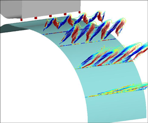
Figure 13 shows the ensemble averaged vortex structures using  $Q$-criteria of the two unforced jet of ${NPR=3.0}$ and $3.9$. In the moderately compressible condition ${NPR=3.0}$ (figure 13a), the streamwise vortices can be observed in the shear layer. According to an analysis of the streamwise vorticity transport equation, our previous work (Wang et al. Reference Wang, Qu, Sun and Bai2023) on the identical configuration and flow condition has revealed that the generation of the streamwise vortices is dominated by the centrifugal instability. The spanwise modulation of the streamwise vortices produces the secondary instability of the shear layer, which leads to the rapid instability and growth of the shear layer. Further, for the compressible flow, the vorticity transport equation is
 \begin{equation} \frac{{\partial \omega }}{{\partial {{t}}}} + u\boldsymbol{\nabla} \omega = \omega \boldsymbol{\nabla} u + \frac{1}{{{\rho ^2}}}\boldsymbol{\nabla} \rho \times \boldsymbol{\nabla} p + \nu \times \Delta \omega, \end{equation}
where  $\omega$ is the vorticity, $u$ the flow velocity, $p$ the local pressure, $\rho$ the local density and $\nu$ the kinematic viscosity coefficient. The second term on the right-hand side is the baroclinic term related to the compressible effect. Figure 14 shows the streamwise vorticity and the contribution of the corresponding baroclinic term at $\theta =25^{\circ }$ of the unforced jet with ${NPR=3.0}$. It can be seen that the baroclinic term has an opposite contribution to the streamwise vorticity in the shear layer, which indicates that the compressibility has the suppression effect on the streamwise vortices. When the convective Mach number increases to 0.88, as shown in figure 13(b), the generation of large-scale streamwise vortices and the growth of the shear layer are considerably inhibited by the highly compressibility effect.

Figure 13. Ensemble averaged vortex structures of the unforced jet using  $Q$-criteria ( $Q=100$, coloured by velocity magnitude): (a) $NPR=3.0, M_c=0.64$; (b) $NPR=3.9, M_c=0.88$.

Figure 14. (a) Streamwise vorticity, and (b) streamwise vorticity arising from the baroclinic term at  $\theta = 25^{\circ }$ (unforced jet, ${NPR=3.0}$).
Furthermore, to evaluate the influence of setting heterogeneities at the nozzle lip, figure 15 shows the ensemble and spanwise averaged Mach contours of different pressure ratios. In these figures, the cylinder Coanda surface has been unfurled into abscissa, that is, the  $x$ axis represents the streamwise direction and the corresponding coordinate value are the azimuth angle of the cylindrical surface from the nozzle exit. Similarly, the ordinate in the figure corresponds to the radial distance from the cylinder surface and has been normalized by the nozzle exit height. For the moderately compressible situation (figure 15a,b), the streamwise vortices induced by centrifugal instability in the unforced jet can destabilize the shear layer rapidly (figure 13a). However, the present of spanwise heterogeneities in the forced jet increases the scope of the shear layer to some extent. In terms of the highly compressible condition (figure 15c,d), the streamwise vortices in the unforced jet are suppressed (figure 13b), which results in a limited growth rate of the shear layer. Once the spanwise distributed protrusions are introduced into the flow, the mixing characteristic of the shear layer is significantly enhanced, that is, the momentum exchange ability is enhanced. The high momentum exchange between the inner and outer sides of the shear layer causes the mainstream velocity of the jet to decrease rapidly, whereas the action region of the shear layer grows significantly.

Figure 15. Ensemble and spanwise averaged Mach contours comparison between forced and unforced jet: (a)  $NPR=3.0, M_c=0.64$ forced jet; (b) $NPR=3.0, M_c=0.64$ unforced jet; (c) $NPR=3.9, M_c=0.88$ forced jet; (d) $NPR=3.9, M_c=0.88$ unforced jet.
In order to quantitively evaluate the development of the unforced and forced jet, figure 16 presents the development of the jet half-width and the shear layer vorticity thickness along the streamwise direction. Compared with the unforced jet, the jet half-width and shear layer vorticity thickness of the forced jet are thickened, indicating that the mixing capacity of the jet shear layer is enhanced. In addition, the location where the jet width and shear layer vorticity thickness begin to grow rapidly advances, suggesting that the shear layer instability has been advanced. This will be further discussed in § 4.2.3.

Figure 16. Ensemble and spanwise averaged (a) jet half-width, and (b) vorticity thickness of the shear layer along the streamwise direction.
Another prominent feature can be seen in figure 16 is that the mixing enhancement in the highly compressible state  $NPR=3.9$ is greater than that in the moderately compressible state $NPR=3.0$. This could be explained by the following two aspects. On the one hand, as compared with the highly compressible condition, the shear layer instability induced by centrifugal instability in the unforced jet is already rather rapid, which leads to a relatively limiting mixing enhancement control effect. On the other hand, a more important aspect is that the jet studied in this paper works in an over expansion state, and there are separations near the nozzle exit. As shown in figure 17, for the moderately compressible state ${NPR=3.0}$, the spanwise distributed protrusions are almost located in the separation region. In comparison, as the pressure ratio increases, the over expansion characteristics of the jet are improved. Consequently, the shock waves in the nozzle are pushed outward, and the associated separation becomes smaller. This enhances the influence of the protrusions on the flow field, thereby increasing the control effect of the mixing enhancement.

Figure 17. Ensemble averaged Mach contours of the forced jet near the nozzle exit: (a)  $NPR=3.0, M_c=0.64$; (b) $NPR=3.9, M_c=0.88$.
4.2. Mechanism of mixing enhancement
4.2.1. Streamwise vorticity in the shear layer
Due to the influence of compressibility, the generation of streamwise vortices in the highly compressible state are suppressed in the unforced jet (figure 13b). However, figure 18 shows the ensemble averaged streamwise velocity development of the forced jet along the streamwise direction. The spanwise distributed protrusions would induce initial instability in the shear layer. This initial instability is subsequently maintained and amplified. In fact, Han et al. (Reference Han, De Zhou and Wygnanski2006) found that similar forcing at the nozzle lip in a plane wall jet did not result in streamwise vortices due to the absence of the centrifugal effects to sustain them. It suggests that the centrifugal effect would be responsible for the amplified initial disturbance.

Figure 18. Ensemble averaged streamwise velocity development along azimuth angles ( $NPR=3.9$, forced jet): (a) $\theta =0^{\circ }$; (b) $\theta =5^{\circ }$; (c) $\theta =15^{\circ }$; (d) $\theta =25^{\circ }$; (e) $\theta =35^{\circ }$; ( f) $\theta =45^{\circ }$.
The mean vorticity transport equation provides a budget of the various effects contributing to a change in the mean vorticity. For a given streamwise location ( ${\theta =\textrm {const}}.$), mean streamwise vorticity arising from the centrifugal effects in a mean term, $CFG(1) = ({1}/{r})({{\partial u_\theta ^2}}/{{\partial z}})$, which is combined with the results of the skewness effect, $\langle {\omega _r}\rangle ({{\partial \langle {u_\theta }\rangle }}/{{\partial r}}) + \langle {\omega _z}\rangle ({{\partial \langle {u_\theta }\rangle }}/{{\partial z}})$, and the curvature effect, $-{{\langle {u_\theta }\rangle \langle {\omega _r}\rangle }}/{r}$. Similarly, the turbulent term, $CFG(2) = ({1}/{r})({{\partial {u'_\theta }^2}}/{{\partial z}})$, accounts for the mean vorticity arising from the turbulent stresses in the flow. Figure 19 shows the ensemble averaged streamwise vorticity at $\theta =45^{\circ }$. The contours of the centrifugal effects in a mean term (figure 19b) show good correspondence with the streamwise vorticity contours (figure 19a), which suggests that the centrifugal effect dominants the streamwise vorticity production. For the centrifugal terms arising from the turbulent stresses (figure 19c), it has a pair of opposite vortices at the position of each streamwise vorticity cell, which would lead to the radial distribution of the streamwise vorticity shifting away from the wall. However, the contribution of this term is one order of magnitude smaller than that of the mean term.

Figure 19. Ensemble averaged streamwise vorticity at  $\theta = 45^{\circ }$ ( $NPR=3.9$, forced jet): (a) streamwise vorticity $(\omega _{\theta}\kern-1pt)$ contours and streamlines; (b) streamwise vorticity due to centrifugal terms arising from the mean flow ( $CFG(1)$); (c) streamwise vorticity due to centrifugal terms arising from the turbulent stresse ( $CFG(2)$).
A further insight into figure 19(a) is that the transportation effect of streamwise vortices produces alternating upwash and downwash regions. This spanwise modulation would trigger the inflection instability of the spanwise flow. The spanwise modulation and associated secondary instabilities lead to the mixing enhancement in a forced jet, which will be discussed in detail in § 4.2.3.
4.2.2. Spanwise wavelength of the streamwise vorticity
In both an unforced and a forced incompressible jet over a convex wall, previous studies have found that the spanwise wavelength scales as twice the local jet half-width (Likhachev et al. Reference Likhachev, Neuendorf and Wygnanski2001; Han et al. Reference Han, De Zhou and Wygnanski2006; Pandey & Gregory Reference Pandey and Gregory2020, Reference Pandey and Gregory2021). As the jet streams downstream and the jet width increases, this relationship is maintained through the streamwise vortex pair merging process. However, the study of Wang et al. (Reference Wang, Qu, Sun and Bai2023) on an unforced compressible convex wall jet indicated that in addition to the convection, diffusion and breaking of the streamwise vortices, no merging process of vortex pairs was observed with the development of jet as well as the increase of jet half-width. In terms of the forced jet here, in order to observe the flow development along the streamwise direction, figure 20 shows the streamwise vorticity, streamwise velocity and radial velocity contours of the stream-span plane  $y/h=1$. The streamwise streaks are caused by the streamwise vortices associated with the centrifugal instability. In the forced jet, the merging phenomenon of the streamwise vortex pair is also not observed. The spanwise wavelength is maintained at a constant value as the forcing wavelength at the nozzle lip, until it breaks into smaller vortices.

Figure 20. Ensemble averaged contours of stream-span plane at  $y/h=1$ ( $NPR=3.9$, forced jet): (a) streamwise vorticity ( $\omega _{\theta }$), (b) streamwise velocity ( $U$), (c) radial velocity ( $V$).
$V$).
Figure 21 shows the streamwise vortices’ distributions in different cross-stream locations. Like the unforced jet, the forced jet is spanwise periodic. Unlike the unforced jet, the spanwise wavelength of the forced jet is consistent with the spanwise distributed forced excitation at the nozzle lip, which is approximately twice the spanwise wavelength of the unforced jet. In addition, the streamwise vortices of the forced jet are stronger and have a wider range of action, especially in the radial direction.

Figure 21. Ensemble averaged streamwise vorticity contours at  $\theta =25^{\circ }$ (a,c,e), and $\theta =45^{\circ }$ (b,d, f). Here (a,b) $NPR=3.0$, unforced jet, (c,d) $NPR=3.0$, forced jet, (e,f) $NPR=3.9$, forced jet.
4.2.3. Streamwise travelling wave
In the boundary layer stability studies (Andersson et al. Reference Andersson, Brandt, Bottaro and Henningson2001; Schlatter et al. Reference Schlatter, Brandt, De Lange and Henningson2008; Konishi & Asai Reference Konishi and Asai2010), the amplitude growth of elongated streamwise streaks due to the lift-up mechanism can develop instabilities. This instability of the streamwise streaks is referred as a secondary instability, which induces the meandering motion of the streamwise vortices. The convection of spanwise meandering motion in the streamwise direction behaves as a streamwise travelling wave. There are four possible modes in this travelling wave including the fundamental sinuous mode, subharmonic sinuous mode, fundamental varicose mode and subharmonic varicose mode (figure 2 in Andersson et al. (Reference Andersson, Brandt, Bottaro and Henningson2001)). In the subharmonic cases, sinuous (varicose) fluctuations of the low-speed streaks are always associated with staggered varicose (sinuous) oscillations of the high-speed streaks. The secondary instabilities are also expected to be active in the shear layer of the convex wall jet. In an incompressible convex wall jet, Pandey & Gregory (Reference Pandey and Gregory2020) revealed the existence of a travelling wave by carrying out POD analysis in the downwash region between two counter-rotating vortices. The conditional averaged results showed that this travelling wave was most consistent with the descriptions of a subharmonic sinuous mode in the boundary layer literature. They also found that the subharmonic sinuous instability is dominant in the incompressible convex wall jet.
In the compressible convex wall jet studied here, figure 22(a) shows the instantaneous streamwise vorticity contours of the unforced moderately compressible case  $NPR=3.0$. The spanwise meandering motion of the streamwise vortices can be clearly observed. This meandering characteristic indicates the presence of streamwise travelling waves in the shear layer. Figure 22(b) shows the schematic of a streamwise travelling sinuous wave. As the wave convects downstream, alternating positive and negative spanwise fluctuation regions are induced. Furthermore, POD analysis is applied to the snapshots of the stream-radial section in the upwash region. Figure 23 presents the eigenvalues (energy) distributions of the POD modes. It is notable that the first two modes have nearly the same eigenvalues. This degeneracy of eigenvalues (eigenvalue pairs) has been demonstrated to be caused by the spatiotemporal symmetries of the flow field (Deane et al. Reference Deane, Kevrekidis, Karniadakis and Orszag1991; Pandey & Gregory Reference Pandey and Gregory2020). Further, spatial distributions of the first two POD modes shown in figure 24 appear virtually as phase-shifted versions of each other, which confirms the presence of the travelling wave. The mode spatial backward tilted pattern is due to the fact that the inner part of the jet flows faster than the outer side. It should be noted that the cylinder Coanda surface has been unfurled into abscissa in these figures.

Figure 22. (a) Instantaneous streamwise vorticity contours at stream-span plane ( $y/h=0.8$, (unforced jet, $NPR=3.0$)), and (b) schematic of a streamwise travelling sinuous wave.

Figure 23. The POD analysis for the spanwise velocity fluctuation of upwash region, POD modes ranked as their eigenvalue (energy) (unforced jet,  $NPR=3.0$).

Figure 24. Spatial distributions of the first two POD modes ( $NPR=3.0$, unforced jet): (a) mode 1; (b) mode 2.
In terms of the forced jet, the spanwise distributed protuberances at the nozzle lip were used to force the initial disturbances and subsequently sustained by the centrifugal effects. The above POD analysis was repeated at two other forced conditions of  $NPR=3.0$ and $NPR=3.9$ that correspond to convective Mach numbers of $M_c=0.66$ and $M_c=0.88$, respectively. Figure 25 shows the eigenvalues (energy) distributions of the POD modes for each forced state. Compared with the unforced jet (figure 23), the eigenvalues of the first two modes are farther apart, which means that the spatiotemporal symmetry of the forced flow is broken to some extent. However, the space distributions of the first two modes shown in figure 26 still exhibit streamwise alternating structures. Moreover, the similar and shifted mode shapes in the streamwise direction confirm the existence of travelling waves in the forced jet.

Figure 25. POD analysis for the spanwise velocity fluctuation of upwash region. POD modes ranked as their eigenvalue (energy): (a)  $NPR=3.0$, forced jet; (b) $NPR=3.9$, forced jet.

Figure 26. Spatial distributions of the first two POD modes: (a) mode 1 ( $NPR=3.0$, forced jet); (b) mode 1 ( $NPR=3.9$, forced jet); (c) mode 2 ( $NPR=3.0$, forced jet); (d) mode 2 ( $NPR=3.9$, forced jet).
The above POD analysis in the stream-radial section of the upwash region reveals the presence of the travelling wave in both the unforced and forced convex wall jet. However, there are four possible modes in this travelling wave instability (Andersson et al. Reference Andersson, Brandt, Bottaro and Henningson2001). The POD analysis of spanwise velocity fluctuation in the stream-span plane can provide insights into the identification of specific travelling wave instability modes. Figure 27 shows the eigenvalues (energy) distributions of the POD modes, the degeneracy of the first two POD eigenvalues confirms the existence of the travelling wave. For the unforced jet, figure 28(a) shows the mean streamwise velocity contour, which represents spanwise alternating high-speed and low-speed streaks. Figure 28(b) shows the spatial distributions of the first POD mode, in which the solid line outlines the sinuous mode instability and the dashed line outlines the varicose mode instability. The varicose type mode is dominated at the early stage of the jet instability, both sinuous and varicose types of disturbances are observed later. It should be noted that even in the same low speed streak, the secondary instability mode may change with the development of the jet. This suggests that there are competitions between different secondary instability modes. In terms of the forced jet, as shown in figure 29, the sinuous type motion seems to dominate due to a sinuous type instability and is more easily excited than the varicose type instability. In fact, Andersson et al. (Reference Andersson, Brandt, Bottaro and Henningson2001) investigated nonlinear evolution of boundary layer streaks, and found that the critical amplitude of the sinuous instability mode is approximately  $26\,\%$ of the free stream velocity, while varicose waves are more stable and have a critical amplitude of approximately $37\,\%$.

Figure 27. POD analysis for the spanwise velocity fluctuation of upwash region. POD modes ranked as their eigenvalue (energy): (a)  $NPR=3.9$, forced jet; (b) $NPR=3.0$, unforced jet.

Figure 28. (a) Mean streamwise velocity contour, (b) spatial distributions of the first POD mode, where solid line outlines the sinuous mode instability and dash line outlines the varicose mode instability ( $NPR=3.0$, unforced jet).

Figure 29. (a) Mean streamwise velocity contour, (b) spatial distributions of the first POD mode, where solid line outlines the sinuous mode instability and dash line outlines the varicose mode instability ( $NPR=3.9$, forced jet).
Another salient feature from comparing figures 24 and 26, as well as figures 28(b) and 29(b), is that the secondary instabilities of the forced jet are excited earlier than those of the unforced jet. In fact, the travelling wave modes of the forced jet are excited near the exit of the jet, while that of the unforced jet does not appear until streamwise location  $\theta =30^{\circ }$. In other words, the secondary instability of the forced jet acts earlier on the shear layer, leading to a rapid instability of the shear layer and thus enhancing the mixing characteristics.
4.3. Turbulence characteristics
According to the analyses above, protrusions at the nozzle lip of the forced jet could trigger initial instability in the shear layer. This initial disturbance will be maintained and amplified downstream by the centrifugal effect, leading to stronger streamwise vortices and earlier instability in the shear layer. In this subsection, the turbulence characteristics of both unforced and forced jet are analysed to present mixing enhancement from the perspective of Reynolds stresses. In order to obtain the two-dimensional (2-D) profiles, the stresses are averaged across the spanwise direction. The local jet half-width  $y_2$ and spanwise averaged maximum streamwise velocity $U_{2Dmax}$ are used as the normalization of length scale and velocity scale, respectively.
In the moderately compressible case ( $NPR=3.0$), figure 30 shows the Reynolds stresses ’development along streamwise locations. The shear stresses $\overline {{u}'{w}'}$ and $\overline {{v}'{w}'}$ are close to zero due to the spanwise average over several wavelengths. For the unforced jet, the Reynolds stresses increase rapidly after $\theta =30^{\circ }$, where instabilities are fully excited by streamwise vortices. Then they exhibit self-similar characteristics after $\theta =60^{\circ }$, where large scale streamwise vortices break into smaller vortices. However, the turbulence stresses in the forced jet are enhanced due to the stronger streamwise vortices and the earlier secondary instabilities induced by the spanwise distributed heterogeneities at the nozzle lip. The maximum turbulent stresses in the shear layer are approximately twice those of the unforced jet. The radial position of maximum fluctuation is closer to the wall (in the normalized sense) owing to stronger streamwise vortices in the forced jet. In addition, the enhanced streamwise vortices and associated instabilities in the forced jet make it more difficult to be in equilibrium, resulting in a continued increase in turbulent stresses downstream and do not achieve self-similarity as unforced jet.

Figure 30. Reynolds stresses development along the streamwise direction ( $NPR=3.0$): (a) $\overline {{u}'^2}/U_{2Dmax}^2$; (b) $\overline {{v}'^2}/U_{2Dmax}^2$; (c) $\overline {{w}'^2}/U_{2Dmax}^2$; (d) $\overline {{u}'{v}'}/U_{2Dmax}^2$; (e) $\overline {{u}'{w}'}/U_{2Dmax}^2$; ( f) $\overline {{v}'{w}'}/U_{2Dmax}^2$.
The Reynolds stresses development of the highly compressible condition ( $NPR=3.9$) are shown in figure 31. In the unforced jet, large-scale streamwise vortices, which respond to the rapid instability of the shear layer, are significantly inhibited by the high compression effect (Wang et al. Reference Wang, Qu, Sun and Bai2023). The absence of the large-scale streamwise vortices leads to a low intensity turbulence fluctuation in the unforced jet shear layer. Moreover, the spanwise normal stress is more suppressed than the streamwise and radial normal stresses, resulting in turbulence anisotropy. In terms of the forced jet, similar to the moderately compressible case, the stresses here are enhanced as a result of instabilities induced by the spanwise distributed heterogeneities. The enhanced turbulent characteristics tend to be isotropic.

Figure 31. Reynolds normal stresses development along the streamwise direction ( $NPR=3.9$): (a) $\overline {{u}'^2}/U_{2Dmax}^2$; (b) $\overline {{v}'^2}/U_{2Dmax}^2$; (c) $\overline {{w}'^2}/U_{2Dmax}^2$; (d) $\overline {{u}'{v}'}//U_{2Dmax}^2$.
5. Conclusions
In this study, the spanwise distributed heterogeneities at the nozzle lip were employed to achieve mixing enhancement in the compressible convex wall jet. The mixing enhancement characteristics and mechanisms were numerically investigated using the DDES method based on the SST turbulence model. In addition, POD was used to gain further insight into the dynamical behaviours of the flow instability mode. The main conclusions are summarized as follows.
(1) In the highly compressible condition, the development of the mean flow show that the jet half-width and the shear layer vorticity thickness growth rates are significantly increased in the forced jet. This indicates that the mixing as well as the momentum exchange of the shear layer is significantly enhanced by setting spanwise distributed heterogeneities at the nozzle lip.
(2) The analysis of the mean vorticity transport equation reveals that the initial perturbations from the spanwise distributed heterogeneities are maintained and amplified by the centrifugal effect, resulting in forced streamwise vortices in the shear layer. The instabilities induced by the streamwise vortices are responsible for the rapid instability and mixing enhancement in the forced jet.
(3) The development of the streamwise vortices show the convection, diffusion and breaking instead of the merging characteristics. The spanwise wavelength of the streamwise vortices is maintained at a constant value, which is consistent with the spanwise distributed forced excitation, until it breaks into smaller vortices. The forced streamwise vortices are stronger and have a wider range of action than that in the corresponding unforced jet.
(4) The spanwise meandering motion of the streamwise vortices is observed in the instantaneous streamwise vorticity contour of the span-radial section. This meandering characteristic indicates the presence of the streamwise travelling waves. The POD analysis carried out in in the upwash region of the stream-radial section shows that the first two modes have nearly the same eigenvalues. This degeneracy of eigenvalues (eigenvalue pairs) and the phase-shifted spatial distributions of the first two POD modes further confirm the presence of the travelling wave.
(5) The POD analysis carried out in the span-radial section provides further insight into the identification of the specific travelling wave instability modes. In the unforced jet, both sinuous and varicose types of disturbances are observed, there would be competition between different secondary instability modes. In terms of the forced jet, the sinuous type motion is dominated because the sinuous type instability is more easily excited than the varicose type instability.
(6) The turbulence stresses in the forced jet are enhanced due to the stronger streamwise vortices and the earlier secondary instabilities induced by the spanwise distributed heterogeneities. The maximum turbulent stresses in the shear layer are approximately twice those of the unforced jet. In the moderately compressible case, the turbulent stresses exhibit self-similar characteristics after
$\theta =60^{\circ }$. Whereas the stresses in the forced jet do not achieve self-similarity due to the enhanced streamwise vortices and associated instabilities, which makes the jet more difficult to be in equilibrium. The highly compressibility effect suppresses the spanwise normal stress more than the streamwise and radial normal stresses, resulting in turbulence anisotropy in the unforced jet. In comparison, the enhanced turbulent characteristics of highly compressible condition tend to be isotropic in the forced jet.

Funding
This study was co-supported by the National Natural Science Foundation of China (no. 11972308 and no. 11902265) and the National Major Basic Research Project 1912.
Declaration of interests
The authors report no conflict of interest.
Data availability statement
The data that support the findings of this study are available from the corresponding author upon reasonable request.


