


1. Introduction
The transport of proteins and biopolymers in biological membranes is an important step in determining their organization (Alberts et al. Reference Alberts, Heald, Johnson, Morgan and Raff2022). Membrane proteins can pass across the bilayer thickness (transmembrane proteins), or interact with one of the leaflets (monotopic proteins). Monotopic proteins can polymerize to form filaments and other higher-order structures that span the micron-scale membrane surface (Baranova et al. Reference Baranova, Radler, Hernández-Rocamora, Alfonso, López-Pelegrín, Rivas, Vollmer and Loose2020; Khmelinskaia et al. Reference Khmelinskaia, Franquelim, Yaadav, Petrov and Schwille2021). In many processes, the protein function is determined by its organization (Shi et al. Reference Shi, Cannon, Curtis, Edelmaier, Gladfelter and Nazockdast2023). Simplified in vitro systems are powerful tools for increasing our physical understanding of complex biological systems, including the organization of membrane proteins. Supported bilayers, rigid beads coated with lipid bilayers, are widely used as a model for spherical cell membranes (Bridges et al. Reference Bridges, Zhang, Mehta, Occhipinti, Tani and Gladfelter2014; Cannon et al. Reference Cannon, Woods, Crutchley and Gladfelter2019; Honerkamp-Smith Reference Honerkamp-Smith2023). The diffusion and transport of these semiflexible filamentous proteins within the fluid membrane are determined, in part, by their hydrodynamic drag. Here, we present the translational and rotational drag of a single filament moving in the top leaflet of a spherical supported bilayer, as a model for studying the transport of rod-like monotopic proteins in the cell membrane. The problem is shown schematically in figure 1. We also discuss how the current formulation and results are easily extendable to transmembrane proteins.

Figure 1. A schematic representation of the problem studied here. A filament is embedded in the outer layer of an incompressible spherical bilayer membrane of viscosity  $\eta _{{m}}$ and surrounded on the exterior side and interior side by 3-D Newtonian fluids of shear viscosity $\eta ^{+}$ and $\eta ^{-}$, respectively. The inner leaflet is a solid sphere of radius $R$. The substrate is separated from the adjacent leaflet with by a thin nanoscopic layer of fluid of depth $H$. Here, $\mu$ is the friction coefficient between the leaflets. The filament dynamics is described by three modes of motions: translation along its axis ( $U_{\parallel }$), translation perpendicular to its axis ( $U_{\perp }$) and rotation around its centre ( $\varOmega$).
A starting point for analysing protein lateral motion in biomembranes is the work of Saffman (Reference Saffman1976) (see also Saffman & Delbrück Reference Saffman and Delbrück1975; Hughes, Pailthorpe & White Reference Hughes, Pailthorpe and White1981), which gives an expression for the drag coefficient of a disk of radius,  $a$, moving in an infinite planar membrane of two-dimensional (2-D) viscosity $\eta _m$, and surrounded with an infinite three-dimensional (3-D) Newtonian fluid of shear viscosity $\eta _f$ on both sides. The coupling between the membrane and 3-D fluid domains introduces the Saffman–Delbrück (SD) length $\ell _0=\eta _m/\eta _f$, which is the length over which momentum transfers from the 2-D membrane to the 3-D bulk fluids. For small particles ( $a/\ell _0\ll 1$), Saffman (Reference Saffman1976) showed that the drag coefficient is only a weak logarithmic function of the disk radius: $\xi _{Saff}=4{\rm \pi} \eta _m(\ln (2\ell _0/a)-\gamma )^{-1}$, where $\gamma$ is the Euler–Mascheroni constant. Saffman's result, and simple extensions of it, have been used to measure the membrane rheology in microrheological experiments; see Molaei et al. (Reference Molaei, Chisholm, Deng, Crocker and Stebe2021), Kim et al. (Reference Kim, Choi, Zasadzinski and Squires2011), Prasad, Koehler & Weeks (Reference Prasad, Koehler and Weeks2006) and chapter 4 of Morozov & Spagnolie (Reference Morozov and Spagnolie2015).
Evans & Sackmann (Reference Evans and Sackmann1988) (see also Sackmann Reference Sackmann1996) extended Saffman's work to a disk moving in a planar membrane that is supported on a rigid boundary. The effect of this boundary is modelled using a Brinkman-like friction term,  $\mu \boldsymbol {u}_m$, in the membrane momentum equation, where $\mu$ is the friction coefficient and $\boldsymbol {u}_m$ is the membrane tangential velocity. The friction introduces a new length scale: ${b}=\sqrt {\eta _m/\mu }$. Stone & Ajdari (Reference Stone and Ajdari1998) considered the case of a planar membrane overlaying a 3-D fluid domain of finite depth, $H$, which similarly introduces a length scale defined as $\ell _H=\sqrt {\ell _0 H}$. The scale, $H$, of the thin film in this set-up is incredibly small, and several experiments have reported that it is around $3\ \text {nm}$ (Bayerl & Bloom Reference Bayerl and Bloom1990; Johnson et al. Reference Johnson, Bayerl, McDermott, Adam, Rennie, Thomas and Sackmann1991) which is comparable to half of the lipid bilayer thickness, $2.5\ \text {nm}$ (Alberts et al. Reference Alberts, Heald, Johnson, Morgan and Raff2022). Moreover, the thickness of the membrane-bound protein is of the same length scale, i.e. the thickness of the septin filament is around $4\ \text {nm}$ (Jiao et al. Reference Jiao, Cannon, Lin, Gladfelter and Scheuring2020).
In both rigid substance supported and overlaying thin film cases, the drag coefficient asymptotes to Saffman's results for small particles ( $a/b\ll 1$ or $a/\ell _{H}\ll 1$), with $b$ or $\ell _H$ replacing $\ell _0$ in the expression for the drag coefficients. Furthermore, in the likely scenario of $b/a\ll 1$ or $\ell _H/a\ll 1$, both models predict a quadratic increase in drag with respect to the particle size ( $\xi \propto \eta _m (a/b)^2$ or $\xi \propto \eta _m (a/\ell _H)^2$). Stone & Masoud (Reference Stone and Masoud2015) used reciprocal theorem and perturbation analysis to compute the drag on a spherical or oblate spheroidal particle moving in the membrane and protruding into the subphase fluid. Zhou, Vlahovska & Miksis (Reference Zhou, Vlahovska and Miksis2022) computed the drag on a sphere in a similar set-up, where the particle is trapped at the interface of two fluids where they considered the effects of the gravity and interfacial deformation.
Levine, Liverpool & MacKintosh (Reference Levine, Liverpool and MacKintosh2004) used a slender-body theory to compute the translational and rotational drag of a rod-like inclusion moving in a planar membrane and adjacent to infinite bulk fluids. They found that , when  $L/\ell_0 \gg 1$, the drag in all directions is dominated by the 3-D fluid viscosity. Specifically, the drag in perpendicular direction scales linearly with the filament length, $\xi_\perp \sim \eta_f L$, while the parallel drag contains an extra weak logarithmic dependency, $\xi_\parallel \sim \eta_f L/\ln (L/\ell_0)$. These predictions were found to be in good agreement with the experiments in the range $0.01 \le L/\ell _0 \le 10$ (Lee et al. Reference Lee, Reich, Stebe and Leheny2010; Klopp, Stannarius & Eremin Reference Klopp, Stannarius and Eremin2017). Fischer (Reference Fischer2004) generalized the work of Levine et al. (Reference Levine, Liverpool and MacKintosh2004), to a planar membrane overlying a fluid domain of finite depth. They found that, when $H/\ell _{0}\ll 1$, the parallel drag grows linearly with $L/\ell _{H}$ while the perpendicular drag grows superlinearly.
Most theoretical studies, including the ones surveyed thus far, consider inclusions that fill the entire membrane thickness. We know that monotopic proteins typically bind to one of the two leaflets in lipid bilayers. Motivated by this observation, Camley & Brown (Reference Camley and Brown2013) computed the drag of a disk embedded in the top leaflet of a planar membrane and surrounded by the infinite 3-D bulk fluid on the outer side and finite bulk fluid on the interior. The two leaflets are coupled through a friction term. They found that the drag monotonically increases with the inter-leaflet friction coefficient, with results matching those of Evans & Sackmann (Reference Evans and Sackmann1988) when the inter-leaflet friction is replaced with the substrate's friction.
While the majority of theoretical studies on the hydrodynamic drag of inclusion in membranes have focused on planar membranes, in most biological applications membranes take a spherical or more complex curved geometry. Henle & Levine (Reference Henle and Levine2010) considered the drag of a disk moving in a spherical membrane that is surrounded by bulk fluids on both sides. They found that the drag follows the results of Saffman & Delbrück (Reference Saffman and Delbrück1975), as long as SD length is replaced with  $\min (\ell _{0},R)$, where $R$ is the radius of the membrane; see also Manikantan (Reference Manikantan2020), Samanta & Oppenheimer (Reference Samanta and Oppenheimer2021) and Jain & Samanta (Reference Jain and Samanta2023) for studies on the surface flow and aggregations induced by force and torque dipoles.
In a recent study, we used slender-body theory to compute the drag of a filament bound to a spherical lipid monolayer immersed in 3-D bulk fluids on the interior and exterior (Shi, Moradi & Nazockdast Reference Shi, Moradi and Nazockdast2022). Our computations show that the closed spherical geometry gives rise to flow confinement effects that increase in strength with an increasing ratio of the filament's length to membrane radius  $L/R$. These effects only cause mild increases in the filament's parallel and rotational resistance; hence, the resistance in these directions can be quantitatively mapped to the results on a planar membrane when the momentum transfer length scale is modified to $\ell ^\star =(\ell _0^{-1}+R^{-1})^{-1}$. In contrast, we find that the flow confinement effects result in a superlinear increase in perpendicular drag with the filament's length when $L/R >1$. These effects are absent in free-space planar membranes.
This study extends our previous work to a filament embedded in the outer leaflet of a bilayer membrane that is supported by a rigid sphere on the interior, as shown in figure 1. We present the conservation equations in § 2 and present the closed-form fundamental solution to a point force in this general geometry in Appendix A. We use these solutions in a slender-body theory to compute the translational and rotational resistance of a filament in § 3. Finally, we summarize and discuss our main findings in § 4.
2. Formulation
We consider a filament of length  $L$, where $\boldsymbol {X}(s)$ is a point located at the $s$ arclength of the filament, embedded in the outer leaflet of a lipid bilayer that is supported on the interior by a rigid sphere of radius $R$. Both leaflets have a 2-D shear viscosity of $\eta _m$. The bilayer is surrounded by a semi-infinite 3-D fluid of viscosity $\eta ^+$ on the exterior. We assume the rigid boundary is separated from the lipid head groups of the bottom leaflet by a thin nanoscopic layer of fluid of viscosity $\eta ^{-}$ (Sackmann Reference Sackmann1996) and depth $H$, as shown in figure 1. The two leaflets are coupled through a friction body force that is proportional to the relative velocity of the two leaflets. We assume the filament curvature is constant along its length and equal to $1/R$ (this is the most likely conformation of the filament if the intrinsic curvature of the filament is smaller than the sphere and the bending forces are much larger than thermal and inter-particle forces), which decouples the translational and rotational motions of the filament, due to geometric and flow symmetries. Thus, the translational resistance tensor is defined as $\boldsymbol{\mathsf{\xi}} =\xi _\parallel ({\partial \boldsymbol {X}}/{\partial {s}})({\partial \boldsymbol {X}}/{\partial {s}})+ \xi _\perp (\boldsymbol{\mathsf{I}}-({\partial \boldsymbol {X}}/{\partial {s}})({\partial \boldsymbol {X}}/{\partial {s}}))$, where $\boldsymbol{\mathsf{I}}$ is the identity matrix and ${\partial \boldsymbol {X}}/{\partial {s}}$ is the tangent vector at the filament centre. The rotational resistance, $\xi _{\varOmega }$, is independent of ${\partial \boldsymbol {X}}/{\partial {s}}$.
Assuming flow incompressibility on the membrane and 3-D fluid domains and negligible inertia, the associated momentum and continuity equations for the membrane and 3-D fluid domains are (Henle & Levine Reference Henle and Levine2010; Samanta & Oppenheimer Reference Samanta and Oppenheimer2021; Shi et al. Reference Shi, Moradi and Nazockdast2022)
 \begin{gather} \eta^{{\pm}}\nabla^{2}\boldsymbol{u}^{{\pm}}-\boldsymbol{\nabla} p^{{\pm}}=\boldsymbol{0},\quad \boldsymbol{\nabla}\boldsymbol{\cdot}\boldsymbol{u}^{{\pm}}=0, \end{gather}
 \begin{gather}\eta_{m}\left(\varDelta_\gamma \boldsymbol{u}_{m}^{{o}} +K(\boldsymbol{x}_m)\boldsymbol{u}_{m}^{{o}}-\frac{1}{b^{2}} (\boldsymbol{u}_{m}^{{o}}-\boldsymbol{u}_{m}^{{i}})\right)-\boldsymbol{\nabla}_\gamma p_{m}^{{o}} +\boldsymbol{T}^{{o}} =\boldsymbol{0},\quad \boldsymbol{\nabla}_\gamma\boldsymbol{\cdot} \boldsymbol{u}_{m}^{{o}}=0, \end{gather}
 \begin{gather}\eta_{m}\left(\varDelta_\gamma \boldsymbol{u}_{m}^{{i}} +K(\boldsymbol{x}_m)\boldsymbol{u}_{m}^{{i}}-\frac{1}{b^{2}} (\boldsymbol{u}_{m}^{{i}}-\boldsymbol{u}_{m}^{{o}})\right)-\boldsymbol{\nabla}_\gamma p_{m}^{{i}} +\boldsymbol{T}^{{i}} =\boldsymbol{0},\quad \boldsymbol{\nabla}_\gamma\boldsymbol{\cdot} \boldsymbol{u}_{m}^{{i}}=0, \end{gather}
where  $\boldsymbol {u}^{\pm }$ and $p^{\pm }$ are the velocity and pressure fields in 3-D fluid domains, and $\boldsymbol {u}_{m}^{{o}}$, $\boldsymbol {u}_{m}^{{i}}$ and $p_{m}^{{o}}$, $p_{m}^{{i}}$ are the velocity and pressure fields in the outer layer and inner layer of the membrane, respectively; $\varDelta _\gamma$ and $\boldsymbol {\nabla }_{\gamma }\boldsymbol {{\cdot }}$ are the surface (defined by $\gamma$) Laplacian and divergence operators, $K$ is the local Gaussian curvature of the surface, $b=\sqrt {\eta _{m}/\mu }$, where $\mu$ is the inter-leaflet drag coefficient, $\boldsymbol {T}^{{o}}=\boldsymbol {\sigma }^{+}(\boldsymbol {x}_m)|_{r=R}\boldsymbol {{\cdot }} \boldsymbol {n}(\boldsymbol {x}_m)$ and $\boldsymbol {T}^{{i}}=-\boldsymbol {\sigma }^{-}(\boldsymbol {x}_m)|_{r=R}\boldsymbol {{\cdot }} \boldsymbol {n}(\boldsymbol {x}_m)$ are the traction applied from the surrounding 3-D fluid domains on the membrane from exterior and interior flow, respectively, where $\boldsymbol {\sigma }^\pm$ denotes the 3-D fluid stress and $\boldsymbol {n}(\boldsymbol {x}_m)$ is the surface normal vector pointing towards the exterior domain.
The boundary conditions (BCs) are the continuity of the velocity and stress fields across all interfaces. The stress continuity is automatically satisfied by adding the traction terms from 3-D fluids to the membrane momentum equations. The velocity and stress fields decay to zero at infinitely large distances from the interface in the outer fluid domain,  $\lim _{r\to \infty } u_{\theta,\phi }^+ (r)\to 0$. Finally, the velocity at the boundary of the supported solid sphere is zero $\boldsymbol {u}_{m}^{{in}}|_{r=R-H}=\boldsymbol {0}$. Since we take the interior to be rigid, the radial velocity becomes exactly zero across all layers and 3-D fluid domains.
The constant Gaussian curvature on the sphere,  $K=R^{-2}$, significantly simplifies (2.1). As a result, we can find closed-form expressions of the Green's function and compute the membrane velocity fields at an arbitrary point $(\theta,\phi )$ in response to a point-force at $(\theta _0,\phi _0)$: $\boldsymbol {u}_m(\theta,\phi )=\boldsymbol{\mathsf{G}}(\theta -\theta _0,\phi -\phi _0)\boldsymbol {{\cdot }} \boldsymbol {f}(\theta _0,\phi _0)$. Here, $\boldsymbol{\mathsf{G}}$ is the Green's function, and $\theta \in [0,{\rm \pi} ]$ and $\phi \in (0,2{\rm \pi} ]$ are the polar and azimuthal angles in spherical coordinates. The detailed derivation of the Green's function and the final expressions are presented in Appendix A.
It is very reasonable to assume that  $H/R\ll 1$ in almost all applications. In Appendix A we show that in this regime the effects of the inner leaflet and the thin fluid layer on the top leaflet can be combined into a single effective friction length scale: $b^{\star }=\sqrt {\ell ^{-}H+b^{2}}$, where $\ell ^{-}=\eta _{m}/\eta ^{-}$. Below, we provide a simple scaling analysis that bears this result.
When  $H/R\ll 1$, the flow inside the thin fluid layer can be approximated as simple shear flow, which results in the associated traction on the bottom leaflet scaling as $\boldsymbol {T}^{i}\sim \eta ^{-} \boldsymbol {u}^{i} /H \sim \eta _m \boldsymbol {u}^{i}/(\ell ^{-} H)$. When the fluid layer thickness is the smallest length scale, the drag from the fluid layer is of the same order of magnitude or larger than the drag force from membrane viscosity: $|\boldsymbol {T}^{i}|\ge |\eta _m \nabla ^2 \boldsymbol {u}_m^{i}|$. Furthermore, we have $K=R^{-2}\ll (\ell ^{-} H)^{-1}$. Thus, in our scaling analysis, we can drop the first two terms in (2.1c) in comparison with $\boldsymbol {T}^{i}$, and we get: $(\boldsymbol {u}^{o}_m-\boldsymbol {u}^{i}_m)/b^2 \sim \boldsymbol {u}^{i}_m/(\ell ^{-} H)$, which gives
 \begin{equation} \boldsymbol{u}^{o}_m \sim \left(1+\frac{b^2}{\ell^{-} H}\right)\boldsymbol{u}^{i}_m. \end{equation}
We now can eliminate  $\boldsymbol {u}_m^{i}$ from (2.1b) by replacing the term $b^{-2}(\boldsymbol {u}_m^{o}-\boldsymbol {u}_m^{i})$ with $(b^\star )^{-2}\boldsymbol {u}_m^{o}$ using the above scaling. Following these steps, we recover $b^\star =\sqrt {\ell ^{-} H +b^2}$. As a result, (2.1) simplify to
 \begin{gather} \eta^{+}\nabla^{2}\boldsymbol{u}^{+}-\boldsymbol{\nabla} p^{+}=\boldsymbol{0},\quad \boldsymbol{\nabla}\boldsymbol{\cdot}\boldsymbol{u}^{+}=0, \end{gather}
 \begin{gather}\eta_{m}\left(\varDelta_\gamma \boldsymbol{u}_{m}^{{o}} +K\boldsymbol{u}_{m}^{{o}}-\frac{\boldsymbol{u}_{m}^{{o}}}{{b^\star}^{2}}\right)-\boldsymbol{\nabla}_\gamma p_{m}^{{o}} +\boldsymbol{T}^{{o}}=\boldsymbol{0},\quad \boldsymbol{\nabla}_\gamma\boldsymbol{\cdot} \boldsymbol{u}_{m}^{{o}}=0. \end{gather}
The BCs are the continuity of the velocity and stress of the outer 3-D fluid and the membrane of the outer layer. Also, 3-D fluid velocity and stress decay to zero at infinitely large distances. Hereafter, the  $\star$ superscript is dropped for brevity.
Since we have a closed-form solution of the Green's function for (2.1) and the more special case of (2.3), we can use slender-body theory to model the flow disturbances induced by a filament with a distribution of force densities. To calculate the resistance in the parallel ( $\xi _\parallel$), perpendicular ( $\xi _\perp$) and rotational ( $\xi _{\varOmega }$) directions, we set the filament velocity(vorticity) as a constant in each direction and compute the distribution of force density on the filament by solving the following integral equation:
 \begin{equation} \boldsymbol{U}(s)= \int_{{-}L/2}^{L/2}\boldsymbol{\mathsf{G}} (\boldsymbol{X}(s)-\boldsymbol{X}(s^\prime))\boldsymbol{\cdot} \boldsymbol{f}(s^\prime)\,\mathrm{d}s^\prime, \end{equation}
where  $\boldsymbol{\mathsf{G}}(\boldsymbol {X}(s)-\boldsymbol {X}(s^\prime ))$ is the Green's function of the membrane–outer 3-D fluid coupled system in response to a point force applied on the membrane at position
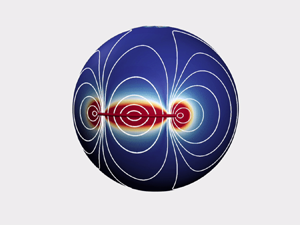
  $\boldsymbol {X}(s^\prime )$. Figure 2 shows the flow fields and colour maps of the velocity magnitudes on the membrane induced by a point force placed at the equator of the top leaflet, when $b/R=10^{-2}$, $1$ and $10^2$, corresponding to weak, intermediate and strong couplings (friction) between the leaflets. In all cases we take $\ell _0/R=1$. Note that the hydrodynamic screening length (the distance over which the velocity decays) is increased with increasing $b/R$ (decreasing friction between the leaflets). Note also that, because of the closedness of the spherical geometry, we obverse two symmetric vortices (recirculation zones) that move further away from the point force as $b/R$ is increased.

Figure 2. The flow field induced by a point force on the equator along the direction of the equator, for the choice of  $\ell _{0}/R=1$ for all cases and $b/R=10^{-2}$, $b/R=1$ and $b/R=10^2$ from left to right. The vector field and the colour map show the direction and magnitude of the flow field, respectively. The vectors’ length is held fixed for better visualization.
The numerical implementations for solving the integral equation (2.4) are given in our earlier work (Shi et al. Reference Shi, Moradi and Nazockdast2022). Integrating the force densities (torque densities) along the filament's length gives the total force (torque), which is equal to the drag in each direction for a unit translational (rotational) velocity. We assume that the filament thickness,  $a$, is negligible compared with all the other lengths. The error of the resistance due to the thickness of the filaments, unlike the filament in 3-D flow, scales with ${O}(\epsilon )$, where $\epsilon =a/L$, and thus, here, we model a filament as an ideal 1-D line; see error analysis in Shi et al. (Reference Shi, Moradi and Nazockdast2022).
Applying a net force to a spherical membrane leads to a net torque on the membrane and its interior, which leads to a rigid-body rotation of the spherical membrane (Henle & Levine Reference Henle and Levine2010; Samanta & Oppenheimer Reference Samanta and Oppenheimer2021). This effect is not present in a planar membrane. The resistance is defined based on the relative velocity of the filament with respect to the ambient fluid:  $\boldsymbol {F}=\boldsymbol {\xi }\boldsymbol {{\cdot }} (\boldsymbol {U}-\boldsymbol {u}^\infty )$, where $\boldsymbol{\mathsf{\xi}} $ is the filament's resistance tensor and $\boldsymbol {u}^\infty$ is the membrane's rotational velocity due to the net torque on it; see details in Appendix A.
2.1. The extension to transmembrane proteins
The formulation we discussed thus far assumes that the protein is monotopic i.e. it only spans the top leaflet of the lipid bilayer and only moves through this layer (figure 1). Here, we discuss how the formulation and the results we are about to present can easily be extended to transmembrane proteins that span both leaflets.
When the protein spans both leaflets, the problem is essentially reduced to a protein moving in a lipid monolayer with twice the thickness of each bilayer leaflet. This lipid monolayer is separated from the supporting surface by a layer of fluid of thickness  $H$. Hence, the results in this limit can be mapped to the results we will discuss in the next sections by (i) taking the membrane 2-D viscosity to be twice as large since the protein motion produces twice as much dissipation within the membrane compared with the case of a protein moving in only one of the leaflets: $\eta _m^{trans} =2\eta _m$; and (ii) by taking $b^\star =\sqrt {\ell ^{-} H}$.
3. Results
3.1. Small inclusions:  $L\ll \min (R,b,\ell ^\pm )$

We begin by examining the drag coefficient of small inclusions, where the largest dimension of the inclusion is significantly smaller than other hydrodynamic length scales in the system:  $L \ll \min (R, H, b, \ell ^\pm )$. In this limit, the drag assumes a general form given by $\xi \approx 4{\rm \pi} \eta _{m}(\ln (2\ell ^{\star }/L))^{-1}$ irrespective of the particle shape, where $\ell ^{\star }$ represents the smallest hydrodynamic length scale in the system, $\ell ^\star =\min (R, H, b, \ell ^\pm )$. The logarithmic term in the drag coefficient arises from the fundamental solution of the 2-D Stokes equation, involving a $\ln (r)$ term that diverges as $r\to \infty$, leading to the well-known Stokes paradox in 2-D Stokes flows. The standard method for resolving this divergence is to account for the mechanical couplings and the resulting momentum transfer between flows inside the membrane and the surrounding fluid domains (Saffman Reference Saffman1976). This momentum transfer from the membrane to the surrounding occurs over lengths that scale with $\ell ^\star$, effectively setting an outer boundary for the membrane.
In the case of a planar membrane surrounded by two unbounded 3-D fluid domains,  $\ell ^{\star } = \ell ^{\pm }$, leading to the original results by Saffman (Reference Saffman1976). In the case of a membrane (or a viscous film) overlaying a 3-D fluid with finite depth, $H$, we get $\ell ^{\star } = \sqrt {\ell ^{-}H}$, as calculated by Stone & Ajdari (Reference Stone and Ajdari1998). For a spherical membrane and when $\ell ^\pm /R\gg 1$, the momentum transfer length is determined by geometrical confinement effects, $\ell ^{\star } = R$, in line with the results of Henle & Levine (Reference Henle and Levine2010). In the case of a drag force resulting from inter-leaflet friction between leaflets or friction between the membrane and substrate, $\ell ^{\star } = b$, consistent with the Evans & Sackmann (Reference Evans and Sackmann1988) results. In summary, the resistance of small inclusions adheres to a general form of the ratio between the inclusion size and the smallest hydrodynamic screening length.
3.2. Two leaflets are strongly coupled
After combining the effect of the thin fluid layer and the bottom leaflet into a single friction coefficient, the filament's drag only depends on four lengths:  $L$,
$L$,  $R$,
$R$,  $\ell ^+=\eta _m/\eta ^+$ and $b^\star$. We begin by considering a strong coupling between the leaflets: $b^\star /\min {(R,\ell ^{+})}\ll 1$. Recall that $b^\star >\max (\sqrt {\ell ^{-}H}, b)$. Hence, in the strongly coupled limit, values of $\max {(b,\sqrt {\ell ^{-}H})}$ are significantly smaller than $\min {(R,\ell ^{+})}$.
Figure 3 shows the computed values of parallel, perpendicular and rotational resistances (drag coefficients) as a function  $L/b$ for different values of $b/\ell ^{+}\ll 1$ and $b/R\ll 1$. We expect the resistance to be determined by the ratio of the filament's length to the shortest hydrodynamic screening length, i.e. $b$. Indeed, all the curves collapse onto a single curve as a function $L/b$ in the parallel, perpendicular and rotational directions as long as $b\ll \min (\ell ^{+}, R)$. In this regime, all the resistance functions converge to the case of a filament embedded in a 2-D planar Brinkman flow, which is plotted as a black line in figure 3. Because $b\ll \min (\ell ^{+}, R)$, the (2.3b) can be simplified into
 \begin{equation} \eta_{m}\left(\varDelta_\gamma \boldsymbol{u}_{m}^{{o}}-\frac{\boldsymbol{u}_{m}^{{o}}}{b^{2}}\right)- \boldsymbol{\nabla}_\gamma p_{m}^{{o}} =\boldsymbol{0},\quad \boldsymbol{\nabla}_\gamma\boldsymbol{\cdot} \boldsymbol{u}_{m}^{{o}}=0, \end{equation}
where  $b^{2}$ plays the same role as the permeability in porous media (Brinkman Reference Brinkman1949). The contributions from the curvature and 3-D bulk flow are negligible when the resistance is dominated by the inter-leaflet friction (Camley & Brown Reference Camley and Brown2013).

Figure 3. The dimensionless parallel (a), perpendicular (b) and rotational (c) drag coefficients as a function of  $L/b$. Grey (circle) and purple (downward triangle) symbols represent different ratios of $b/\ell ^{+}$, while $\ell ^{+}/R=1\times 10^{-2}$ was kept fixed. Blue (square) and green (leftward triangle) represent different ratios of $b/R$ while $\ell ^{+}/R=1\times 10^{2}$ was kept fixed. The solid black lines are the associated resistance values of Brinkman flow in planar membranes, where the $x$-axis is $L/\sqrt {\kappa }$ and $\kappa$ is the permeability of the porous medium.
Note that we have only presented the results for  $L/b \ge 1$. For $L/b<1$, the drag is dominated by the membrane shear stresses and the drag, as expected, asymptotes to Saffman's formulae with $b$ replacing $\ell _0$: $\xi _{\perp,\parallel }\approx 4{\rm \pi} \eta _m \ln ^{-1}(b/L)$.
When,  $L/b\gg 1$, the parallel and perpendicular resistances exhibit a linear and quadratic dependency with $L$:
$L$:  $\xi _{\|}\propto {L/b}$ and $\xi _{\perp }\propto {(L/b)^{2}}$. To explain this scaling, let us first assume the force distribution along the filament is nearly uniform due to its high aspect ratio. As a result, the filament's mobility scales as
 \begin{equation} \chi_{{\parallel},\perp}=\xi_{{\parallel}, \perp}^{{-}1} \sim \frac{1}{L}\int_0^{L} G_{{\parallel}, \perp} (r)\,{\rm d} r. \end{equation}
Furthermore, the integral of the Green's function of a 2-D Brinkman flow satisfies the following asymptotic relationships (Kohr, Sekhar & Blake Reference Kohr, Sekhar and Blake2008; Gradshteyn & Ryzhik Reference Gradshteyn and Ryzhik2014):
 \begin{equation} \lim_{\tilde{r}\to \infty} \int_{0}^{\tilde{r}} G_{\|}(r)\,{\rm d} r = {\rm \pi}-2/\tilde{r},\quad \lim_{\tilde{r}\to \infty} \int_{0}^{\tilde{r}}G_{{\perp}}(r)\,{\rm d} r=2/\tilde{r}. \end{equation}
Thus, when  $L/b\gg 1$, the filament's mobility scales with
 \begin{equation} \xi^{{-}1}_{\|}\sim\frac{b}{L}\int_{0}^{L/b}G_{\|}(\tilde{r})\,{\rm d}\tilde{r}={O}(b/L),\quad \xi^{{-}1}_{{\perp}}\sim\frac{b}{L}\int_{0}^{L/b}G_{{\perp}}(\tilde{r})\,{\rm d}\tilde{r}={O}(b/L)^{2}, \end{equation}
where  $\tilde {r}=r/b$. This scaling leads to the linear and quadratic growths of the resistances in the parallel and perpendicular directions, respectively. These scaling results are analogous to those reported by Fischer (Reference Fischer2004), who computed the translational drag of a needle moving in a planar lipid monolayer and overlaying a thin fluid layer of thickness $H$. This is expected since, in the strong coupling regime, the fluid flows and their associated drags become independent of membrane curvature and identical to planar membranes. Furthermore, in this regime, the frictional forces from the thin fluid layer in Fischer (Reference Fischer2004) can be modelled by a Brinkman-like term, which leads to an identical form of the equations of motion in both problems.
The rotational resistance also scales quadratically with the filament's length,  $\xi _{\varOmega }\propto {(L/b)^{2}}$, since filament rotation involves moving perpendicular to its axis.
To gain a better physical understanding of these scaling relationships it is useful to study the the velocity field generated by the filament motion. Figure 4 shows the flow streamlines for parallel, perpendicular and rotational motions. The colour map underlying the streamlines shows the velocity (vorticity) magnitude on the spherical surface when normalized by the net velocity (vorticity) of the filament. These results are presented for the choice  $L/R=1$, $\ell ^+/R=1$ and $b/R=0.1$. As can be seen in the left column of figure 4, the velocity magnitude decays to zero very rapidly around the filament moving in the parallel direction; see also the dashed contour corresponding to $|\boldsymbol {u}_m|=0.5$. An inspection of the flow fields shows that the velocity fields decay over distances that scale with $b$. Thus, we can approximate the system as a rectangle with $L\times b$ hydrodynamic dimensions moving with velocity $U_\parallel$. Given that the traction from membrane flow gradients scales with membrane velocity magnitude, and that these gradients are very small outside of the rectangle, we can safely ignore those contributions to the drag compared with the traction from the bottom leaflet/substrate. As a result, the total drag force on the rectangle is simply the integral of the substrate traction, $f=\eta _m U_\parallel /b^2$, over the area of the rectangle, $L\times b$. So we get $F_\parallel \approx (Lb) \eta _m U_\parallel /b^2= \eta _m U (L/b)$, which yields $\xi _\parallel =F/U_\parallel \sim \eta _m (L/b)$.

Figure 4. The interfacial flow field induced by filament motion in the parallel (a,d), perpendicular (b,e) and rotational (c,f) directions, when  $\ell ^{+}/R=1$, $L/R=1$ and $b/R=0.1$. The scale for the filament's translational rotational velocity is set to be 1. The white lines represent the streamlines and the underlying heat map represents the magnitude of the fluid velocity (a,b) and vorticity (c). The upper row shows the zoomed-in velocity (left and middle) and vorticity (right) fields close to the filament, where the black dashed lines represent the contour of velocity $\lvert \boldsymbol {u}_{m}\rvert =0.5$ and vorticity $\lvert \boldsymbol {\varOmega }_{m}\rvert =0.5$.
The middle row of figure 4 shows the streamlines and the colour maps of velocity magnitude when the filament moves perpendicular to its axis. Notice that, unlike the velocity fields for parallel motion, the velocity magnitudes remain of  ${O}(1)$ over distances that scale with the length of the filament. Hence, the effective dimensions of the filament scale as $L\times L$. Following the same line of argument as in parallel motion, we can approximate the total drag from inter-leaflet frictional forces as $F_\perp \sim (L^2)\eta _m U_\perp /b^2$, which gives $\xi _\perp \sim \eta _m (L/b)^2$.
We note that the parallel and perpendicular drag has the same scaling law as the filament moving in a supported planar monolayer (Fischer Reference Fischer2004). This is a consequence of the fact that the effects of curvature and exterior fluid are negligible and thus the resistances are the same as long as  $\ell ^{-}H$ in Fischer (Reference Fischer2004) is substituted for $b^{2}$ in this work. Moreover, the perpendicular drag has the same form as the drag of a disk of size $L$ when $L/b \gg 1$ (Evans & Sackmann Reference Evans and Sackmann1988; Sackmann Reference Sackmann1996). It is easy to explain this similarity by noting that the effective hydrodynamic dimensions of a filament of length $L$ are the same as a disk of the same diameter. The same line of argument can be used to explain why we observe the same scaling for the rotational drag as well: $\xi _\varOmega \sim \eta _m (L/b)^2$.
3.3. The drag coefficients in supported bilayers vs vesicles
The plasma membrane is attached to the underlying cell cortex through a variety of cross-linkers (Itoh & Tsujita Reference Itoh and Tsujita2023). Depending on the strength of these attachments and the cellular context, the membrane can be nearly decoupled or fully coupled from the cell cortex. When the membrane is weakly cross-linked to the cell cortex, it is more analogous to a vesicle. Hence, vesicles are also widely used a models for synthetic cells (Walde Reference Walde2010). In contrast, when the membrane is strongly cross-linked to the cell cortex it is more accurately represented as a supported bilayer. In this section, we explore the ratio of the drag coefficients in vesicles and supported bilayers, to gain a better understanding of the difference in protein transport in these two model systems for the cell membrane.
The derived Green's function for (2.1) applies to arbitrary values of  $R, H$, and $\ell ^\pm$ in their accepted physical range. Thus, we can compute the drag of a filament moving in the outer leaflet of a vesicle, $\xi ^{vsc}$, by setting $H=R$ in the Green's function and solving (2.4). We have performed these calculations for the same values of $\ell ^+$, $R$ and $b$ that are reported in figure 3, but with $H=R$. For simplicity, we assumed the interior and exterior fluids have the same viscosity i.e. $\ell =\ell ^+=\ell ^-=\eta _m/\eta ^{\pm }$.
In an earlier study, we computed the drag on a filament moving in a suspended lipid monolayer (lipid monolayers, such as the Langmuir monolayer, are widely used as models for biomembranes Stefaniu, Brezesinski & Möhwald Reference Stefaniu, Brezesinski and Möhwald2014), where we assumed the same 3-D viscosity on the interior and exterior (Shi et al. Reference Shi, Moradi and Nazockdast2022). As we show in the next section, the ratio of the computed drag of a filament moving in a vesicle to the drag of the same filament moving in a monolayer membrane of the same composition and viscosity remains in the range [0.5–2], over the entire parameter space of  $R, b, \ell ^\pm$ and $L$; consequently, the drag coefficients in both systems have the same scaling with the filament's length. Here, we focus on the large differences between supported vs vesicles/monolayer. We discuss the ${O}(1)$ variations of drag coefficients between vesicles and lipid monolayers in the next section.
The scaling relationships of the filament's drag embedded in a monolayer/vesicle are summarized in table 1. When the filament's length,  $L$, is smaller than $\ell ^{\star }=\min (\ell _{0},R)$, the drag converges to the results of Saffman (Reference Saffman1976), with $\ell ^\star$ replacing $\ell _0$ as the shortest hydrodynamic screening length. When $\ell _{0}\ll {L}< R$, the drag asymptotes to the drag of a long filament, $L/\ell _0 \gg 1$, embedded in a planar membrane (Levine et al. Reference Levine, Liverpool and MacKintosh2004). Finally, when the filament length is larger than the sphere radius, $L>R$, the closed spherical geometry gives rise to flow confinement effects that lead to an increase in the perpendicular drag and superlinear scaling with $L/\ell ^\star$; these flow confinement effects are significantly weaker in the parallel and rotational directions.
Table 1. The scaling behaviour of dimensionless drag coefficients of a rod-like particle of length  $L$ moving in suspended lipid monolayer and bilayers (vesicles). Here, $\ell ^{\star }=\min (\ell _{0},R)$ and $1<\alpha \le 2$; $\hat {\xi }_{\parallel, \perp } =\xi _{\parallel, \perp }/4{\rm \pi} \eta _m$ and $\hat {\xi }_{\varOmega } =\xi _{\varOmega }/4{\rm \pi} \eta _m L^2$.

We can now study the changes in the ratio of the filament's drag in supported and suspended spherical membranes as a function of the other ratios of the physical lengths in the system. We present the results for both the small sphere and large sphere limits, by taking  $\ell ^{+}/R=1\times 10^2$ and $\ell ^{+}/R=1\times 10^{-2}$, respectively. First, let us consider the special case of nearly zero friction, $b\to \infty$. In this limit, the bottom leaflet of both systems will remain stationary (no flows in the bottom leaflet), and the drag is entirely determined by the flows in the top leaflet and the outer 3-D fluid domain. These flows, and their associated drag, are identical in both systems, resulting in the ratio of $\xi ^{spp}/\xi ^{vsc}\approx 1$, when $b\to \infty$, irrespective of the other parameters.
3.3.1. The small sphere limit, $\ell ^+/R\gg 1$

In the small sphere limit, the drag in all directions becomes nearly independent of  $\ell ^{+}$ and only a function of $L/R$ and $b/R$. Figure 5 shows the ratio of drag coefficients vs $L/R$ in the parallel, perpendicular and rotational directions. The results are presented for a wide range of $b/R$ ratios. When $b/R>1$, the inter-leaflet coupling is weak and, as we discussed earlier, the ratios remain close to one in all directions.

Figure 5. The ratio of the parallel (a,d), perpendicular (b,e) and rotational (c,f) drag of a filament moving in the outer layer of a spherical supported bilayer to the drag of the same filament in a vesicle (freely suspended bilayer) as a function of the ratio of the filament's length to the membrane radius,  $L/R$. (a–c) Show the results for the small sphere case, $\ell ^{+}/R=1\times 10^2$, where the drag becomes nearly independent of $\ell ^{+}$. (d–f) Show the results for the large sphere case. The dashed lines are the fits corresponding to $y=a\log (x)+b$, $y=ax+b$ and $y=ax^{2}+b$ in the left (a,d), middle (b,e) and right (c,f) columns, respectively. Variables $a$ and $b$ are fitting coefficients. The insets show the deviation of the scaling laws as the filament length is increased to $L/R>1$. The dashed lines in the insets are the same lines as the main figure. The dash dotted lines in the inset of figure 5(c) is a linear function, $y=ax+b$.
As shown in figure 5(a), the ratios of parallel drag strongly increase with decreasing  $b/R$. When $b/R\ll 1$, we observe a logarithmic scaling of the ratios with $L/R$ (see the dashed lines in figure 5a). This scaling can be explained by recalling that $\xi _{\parallel }^{spp} \sim L/b$ and $\xi _{\parallel }^{vsc}\sim (L/R)(\ln (L/R))^{-1}$, which makes their ratio scale as $\xi _{\parallel }^{spp}/\xi _{\parallel }^{vsc} \sim (b/R)^{-1}\ln (L/R)$.
Figure 5(b) presents the drag ratios vs  $L/R$ in the perpendicular direction for the same values of $b/R$. Again, the ratios reduce to $1$ for weak couplings of the two leaflets ( $b/R> 1$). We also observe a strong increase in the drag ratios with decreasing $b/R$ with these increases being stronger than the parallel case (compare the values corresponding to $b/R=1\times 10^{-3}$ in both cases). The ratio $\xi _{\perp }^{spp}/\xi _{\perp }^{vsc}$ shows a linear scaling with $L/R$ when $L/R<1$, compared with the logarithmic scaling we observed for the parallel drag; see the dashed lines in figure 5(b). This scaling can similarly be explained by noting that $\xi _{\perp }^{spp} \sim (L/b)^2$ and $\xi _{\perp }^{vsc}\sim (L/R)$. Thus, we have $\xi _{\parallel }^{spp}/\xi _{\parallel }^{vsc} \sim (b/R)^{-2} (L/R)$. As a result, for a fixed value of $L/R$, the ratio increases as $(b/R)^{-2}$, and for a fixed $b/R$, the ratio scales as $L/R$.
The insets of figure 5(b) show that, when  $L/R>1$, the drag ratios begin to deviate from the linear scaling and reach a plateau for different values of $b/R$. To explain this behaviour we recall that flow confinement effects lead to superlinear growth of the perpendicular drag with $L/R$ in vesicles. As a result, $\xi _{\perp }^{supp}/\xi _{\perp }^{vsc}\sim (L/R)^{2-\alpha }$ with $1<\alpha \le 2$.
Figure 5(c) shows the rotational resistance ratios vs  $L/R$. As we discussed earlier, when $L/R<1$ (or more generally, when $L/\ell ^\star <1$), $\xi _{\varOmega }^{vsc} \sim {O}(1)$ (see table 1), while $\xi _\varOmega ^{spp} \sim (L/R)^2$. Thus, we get $\xi _\varOmega ^{spp}/\xi _\varOmega ^{vsc} \sim (L/R)^2$. This trend is shown with the fitted dashed lines of the form $y=ax^2+b$ in the same figure. When $L/R>1$, $\xi _{\varOmega }^{vsc} \sim (L/R)$, which results in a linear scaling of the ratio. This is shown as the dashed dotted lines in the insets of figure 5(c).
3.3.2. The large sphere limit, $\ell ^+/R\ll 1$

Figure 5(d–f) shows the the drag ratio in the large sphere limit,  $\ell ^{+}/R=1\times 10^{-2}$. The scaling laws are the same as in the small sphere limit, with $\ell ^{+}$ substituting $R$ in these figures. Note that the flow confinement effects at $L/R>1$ lead to superlinear growth in the filament's drag with length in the vesicle system. This corresponds to $L/\ell ^{+}>1\times 10^{2}$ assuming $\ell ^{+}/R=1\times 10^{-2}$.
Note also that, as shown in figure 5(f), the drag ratio in the rotational direction scales linearly with  $L/\ell ^+$. In comparison, as shown in figure 5(c), we observe a quadratic scaling of this ratio in the small sphere limit when $L/R<1$, changing to a linear scaling when $L/R>1$. This difference between the small sphere and large sphere limits can be explained by examining the drag on a vesicle/monolayer in different regimes of $L/\ell ^\star$, where $\ell ^\star =\min (R, \ell ^+)$. These regimes are listed in table 1.
The rotational drag in a vesicle/monolayer is of  ${O}(1)$ when $L/\ell ^\star <1$, and scales linearly with $L/\ell ^\star$ when $L/\ell ^\star >1$. Since all the results presented in figure 5(f) correspond to $L/\ell ^+>1$ and the rotational drag on a supported bilayer scales as $(L/\ell ^\star )^2$, we observe a linear scaling ratio of the rotational drags in this range of parameters. In comparison, in the small sphere case where $0.1< L/R\le 2$, the drag ratio scales as $(L/R)^2$ when $L/R<1$, and scales as $L/R$ when $L/R>1$.
3.4. The drag coefficients in vesicles vs lipid monolayers
Next, we present the computed ratios of the filament's drag in a bilayer vesicle vs a Langmuir monolayer in the parallel, perpendicular and rotational directions. We assume the thickness and viscosity for each leaflet of the bilayer is the same as the monolayer with the same 3-D fluid viscosity in both systems. The drag in both cases is the sum of the forces applied from the 2-D membrane flows and the surrounding 3-D flows:  $\xi =\xi _m+\xi ^+_f+\xi ^-_f$, where superscripts $+$ and $-$ refer to the outer and inner fluids, respectively. Thus, we have
 \begin{equation} \frac{\xi^{vsc}}{\xi^{mono}}=\frac{\xi^{vsc}_m+\xi^{{vsc},+}_f+\xi^{{vsc},-}_f}{\xi_m^{mono}+ \xi^{{mono},+}_f+\xi^{{mono},-}_f}. \end{equation}
3.4.1. Small sphere limit, $\ell ^+/R\gg 1$

Figure 6(a–c) shows the computed ratios in the small sphere limit:  $\ell ^{+}/R=1\times 10^2$. As shown in table 1, the dimensionless drag in the monolayer and the vesicle scales only with $L/R$, which makes the drag proportional to $\eta _m$ and independent of the viscosity of the 3-D fluids i.e. $\xi ^{\pm,{vsc}}=\xi ^{\pm,{mono}} \approx 0$, which yields
 \begin{equation} \lim_{\ell^+{/}R \to \infty} \frac{\xi^{vsc}}{\xi^{mono}}\approx \frac{\xi_m^{vsc}}{\xi_m^{mono}}. \end{equation}
When  $b/R \to \infty$, the vesicle's inner leaflet does not move in response to the filament's movement in the outer leaflet. As a result, the membrane flow and the resulting drag on the filament moving in a vesicle become identical to the those in a lipid monolayer. Hence, we observe a ratio $1$ of the drag coefficients when $b/R\to \infty$ for all values of $L/R$ and in all directions of motion.

Figure 6. The ratio of the parallel (a,d), perpendicular (b,e) and rotational (c,f) drag of a filament moving in the outer layer of a vesicle to the drag of the same filament in a lipid monolayer. (a–c) Represent the small sphere limit where  $\ell ^{+}/R=1\times 10^2$, and (d–f) represent the large sphere limit where $\ell ^{+}/R=1\times 10^{-2}$.
When  $b/R \to 0$, leaflets co-move with the same velocity. As a result, the dissipation, and thus the drag, generated by moving a filament in a vesicle with two layers becomes twice as large as the drag of a filament moving with the same velocity in a lipid monolayer. Thus, the drag ratios approach $2$, irrespective of $L/R$.
The drag ratio at the intermediate values of  $b/R$ is a function of $L/R$. Our results suggest that increasing $L/R$ leads to monotonic increases in the drag ratios in all directions and for all values of $b/R$. A more careful analysis of the generated flows and the Green's function is needed to explain these variations, which is outside of the scope of this work.
3.4.2. Large sphere limit, $\ell ^+/R\ll 1$

Next, we discuss the results of drag ratios in the large sphere limit,  $\ell ^{+}/R=1\times 10^{-2}$, presented in figure 6(d–f), where the dimensionless drag coefficients become independent of $L/R$ and only functions of $L/\ell ^+$ in all directions; see table 1. Re-writing the drag coefficients in dimensional form in the regime $L/\ell ^+ \gg 1$ gives the following scalings with the membrane and the 3-D fluid viscosities:
 \begin{equation} \xi_\parallel\sim \eta_f/\ln ( \eta_f /\eta_m),\quad \xi_\perp \sim \eta_m^{1-\alpha} \eta_f^\alpha,\quad \xi_\varOmega \sim \eta_f. \end{equation}
 As this scaling analysis shows, aside from the rotational drag in the limit of  $L/\ell ^+\gg 1$, the drag of a filament in a lipid monolayer or a vesicle in the large sphere limit is a function of both the membrane and 3-D fluid viscosities. This makes it difficult to explain the variations of the drag ratios in terms of simple scaling arguments. However, it is still possible to explain why the ratio satisfies the following inequality: $0.5\le {\xi ^{vsc}}/{\xi ^{mono}}\le 2$.
The case of  $b/\ell ^+ \gg 1$: in this limit, the vesicle's inner leaflet does not move, leading to a negligible contribution of this layer to the drag. In the large sphere limit, we expect only small contributions of sphere curvature to the overall 3-D flows; thus, the contributions to the drag from the outer and inner fluids in the lipid monolayer should be nearly equal: $\xi ^{+,{mono}}_f=\xi ^{-,{mono}}_f$. We also expect identical membrane and outer 3-D flows in the monolayer and the vesicle system, which means $\xi ^{vsc}_m=\xi ^{mono}_m=\xi _m$. Considering all these effects, (3.5) simplifies to
 \begin{equation} \lim_{\substack{\ell^+{/}R \to 0 \\ b/\ell^+\to \infty}} \frac{\xi^{vsc}}{\xi^{mono}}=\frac{\xi_f^++ \xi_m}{2\xi_f^++\xi_m}. \end{equation}
When  $\xi _m\ll \xi _f^+$, the ratio asymptotes to $1/2$. When the drag is dominated by the membrane viscosity ( $\xi _m \gg \xi _f^+$), the ratio approaches $1$.
$1$.
The case of  $b/\ell ^+ \ll 1$: in this case, both layers move with the same velocity. As we discussed in the prior section, we expect twice as much dissipation and drag contributions from the membrane in the vesicle system, compared with the lipid monolayer. Following the same line of reasoning, (3.5) simplifies to
 \begin{equation} \lim_{\substack{\ell^+{/}R \to 0 \\ b/\ell^+\to 0}} \frac{\xi^{vsc}}{\xi^{mono}}=\frac{2\xi_f^+ + 2\xi_m}{2\xi_f^++\xi_m}. \end{equation}
Thus, in the limit of negligible drag from the membrane, the ratio approaches  $1$. If both the membrane and 3-D fluids contribute equally to the drag, $\xi _f^+=\xi _m$, the ratio increases to $4/3$, and if the drag is dominated by membrane flows, the ratio again asymptotes to $2$. In reality, the relative contribution of membrane flows to the overall drag is a complex function of the exact values of $b/\ell ^+$, $L/\ell ^+$ and $L/R$. However, as we showed here, the ratio remains bound in the range [0.5–2], in the wide range of parameters studied here.
4. Summary
The transport and assembly of rod-like proteins and cytoskeletal filaments on biological membranes occur in many cellular processes. A widely used in vitro set-up for studying protein–membrane interactions involves coating rigid beads of comparable size to the cell with lipid bilayers, as models for the cell membrane. Different aspects of the protein structure and dynamics can be measured over time using different microscopy techniques (Cannon et al. Reference Cannon, Woods, Crutchley and Gladfelter2019). As previous studies on planar-supported membranes have shown (Sackmann Reference Sackmann1996), the presence of a rigid substrate qualitatively changes the tangential flows and the resulting hydrodynamic drag of the inclusions. However, except for a few studies (Levine et al. Reference Levine, Liverpool and MacKintosh2004; Henle & Levine Reference Henle and Levine2010), these studies have been limited to disk-like particles and planar membranes. This work fills some of the gaps in the literature by computing the drag of a single filament in a supported spherical bilayer, using a slender-body formulation.
Furthermore, the formulation presented here combines the effects of membrane curvature, inter-leaflet friction of lipid bilayers and the depth and viscosity of the surrounding 3-D domains into a unified theoretical framework. The derived Green's function can also be used in domain integral methods (Camley & Brown Reference Camley and Brown2013) to compute the drag of inclusions of arbitrary shape, and to simulate the dynamics assembly of proteins on supported spherical membranes.
To summarize, our results show that the presence of the rigid substrate influences the filament's dynamics in several distinct ways. When the two leaflets of the bilayer are strongly coupled, the drag becomes independent of membrane radius and SD length and only a function of the inter-leaflet friction length scale,  $b$. We find that the drag in the parallel direction scales linearly with the filament's length, while the perpendicular and rotational drags scale quadratically with length; see details in figure 3. We explained this scaling using the analytical form the Green's function for a point force on the membrane, and by visualizing the velocity fields around the filament undergoing parallel, perpendicular and rotational motions; see figure 4.
We compute the ratio of the drag in supported bilayers to that in freely suspended vesicles,  $\xi ^{spp}/\xi ^{vsc}$. When inter-leaflets are weakly coupled, the drag in all directions asymptotes to the drag on lipid monolayers and vesicles. Increasing the inter-leaflet friction leads to significant increases in the ratio of drag coefficients, particularly in the perpendicular and rotational directions. We explained these variations in terms of the scaling between $\xi ^{spp}$ vs $b/R$ and $\xi ^{vsc}$ vs $L/R$ for the parallel, perpendicular and rotational drag coefficients.
The measurement of membrane viscosity has been conducted over decades by many different experimental methods and simulations. The reported values vary within the range  $\eta _{m}\in [10^{-10}, 10^{-6}]\,(\mathrm {Pa}\,\mathrm {s}\,\mathrm {m})$, depending on lipid composition (Block Reference Block2018; Sakuma et al. Reference Sakuma, Kawakatsu, Taniguchi and Imai2020; Nagao et al. Reference Nagao, Kelley, Faraone, Saito, Yoda, Kurokuzu, Takata, Seto and Butler2021). In comparison, fewer studies have been conducted to quantify the inter-leaflet friction coefficients (Pott & Méléard Reference Pott and Méléard2002; den Otter & Shkulipa Reference den Otter and Shkulipa2007; Jonsson et al. Reference Jonsson, Beech, Tegenfeldt and Hook2009; Blosser et al. Reference Blosser, Honerkamp-Smith, Han, Haataja and Keller2015; Botan et al. Reference Botan, Joly, Fillot and Loison2015; Zgorski, Pastor & Lyman Reference Zgorski, Pastor and Lyman2019; Amador et al. Reference Amador, Van Dijk, Kieffer, Aubin-Tam and Tam2021). The reported values vary in the wide range of $\mu \in [10^{0}, 10^{9}]\,(\mathrm {Pa}\,\mathrm {s}\,\mathrm {m}^{-1})$. The recent study by Amador et al. (Reference Amador, Van Dijk, Kieffer, Aubin-Tam and Tam2021) shows that the friction coefficient can change by orders of magnitude with changes in membrane composition.
Our results suggest another method of measuring inter-leaflet friction and membrane viscosity in the likely condition that the inter-leaflet friction length is the smallest hydrodynamic length of the system,  $b\ll \min (\ell _0,R)$. In this limit, the dimensionless drag in the perpendicular direction scales as $\xi _{\perp }/(4{\rm \pi} \eta _{m})\sim (L/b)^2$. Since $b^2=\eta _m/\mu$, we get $\xi _\perp \sim \mu L^2$ i.e. the perpendicular drag is independent of membrane viscosity and only a function of the filament's length and inter-leaflet friction coefficient. Applying the same analysis to parallel drag gives the following scaling: $\xi _{\|}\sim L\sqrt {\mu \eta _{m}}$. The drag coefficients in all directions can be measured by tracking the position and orientation of rod-like proteins and applying the fluctuation–dissipation Theorem. The measured drag coefficients can then be used to compute the inter-leaflet friction and the membrane viscosity.
Funding
This study is supported by National Science Foundation under career grant no. CBET-1944156.
Declaration of interests
The authors report no conflict of interest.
Appendix A
Here, we outline the fundamental solutions to the system of (2.1) in response to a point force,  $\boldsymbol {f}^{ext}$, on the membrane at position $(\theta _0,\phi _0)$ on the outer layer of the sphere, where $\theta \in [0,{\rm \pi} ]$ is the polar angle and $\phi \in [0,2{\rm \pi} )$ is the azimuthal angle, defined in figure 1. The equations after including the externally applied point force are
 \begin{gather} \eta^{{\pm}}\nabla^{2}\boldsymbol{u}^{{\pm}}-\boldsymbol{\nabla} p^{{\pm}}=\boldsymbol{0}, \end{gather}
 \begin{gather}\boldsymbol{\nabla}\boldsymbol{\cdot}\boldsymbol{u}^{{\pm}}=0, \end{gather}
 \begin{gather}\eta_{m}\left(\varDelta_\gamma \boldsymbol{u}_{m}^{{out}} +K\boldsymbol{u}_{m}^{{out}}-\frac{1}{b^{2}}(\boldsymbol{u}_{m}^{{out}}- \boldsymbol{u}_{m}^{{in}})\right)-\boldsymbol{\nabla}_\gamma p_{m}^{{out}} + \boldsymbol{T}^{{out}}|_{r=R}+\boldsymbol{f}^{{ext}}{\delta} (\theta_0,\phi_{0})=\boldsymbol{0}, \end{gather}
 \begin{gather}\boldsymbol{\nabla}_\gamma\boldsymbol{\cdot} \boldsymbol{u}_{m}^{{out}}=0, \end{gather}
 \begin{gather}\eta_{m}\left(\varDelta_\gamma \boldsymbol{u}_{m}^{{in}} +K\boldsymbol{u}_{m}^{{in}}-\frac{1}{b^{2}}(\boldsymbol{u}_{m}^{{in}}- \boldsymbol{u}_{m}^{{out}})\right)-\boldsymbol{\nabla}_\gamma p_{m}^{{in}} + \boldsymbol{T}^{{in}}|_{r=R}=\boldsymbol{0}, \end{gather}
 \begin{gather}\boldsymbol{\nabla}_\gamma\boldsymbol{\cdot} \boldsymbol{u}_{m}^{{in}}=0, \end{gather}
where  $\delta (\theta _0,\phi _0)$ is the Dirac delta function. The analytical solution to suspended spherical lipid monolayers was provided by Henle & Levine (Reference Henle and Levine2010). Here, we extend their results to solve for the (A1). The velocity field at an arbitrary point $(\theta,\phi )$ in the outer layer is $\boldsymbol {u}(\theta,\phi )=\boldsymbol{\mathsf{G}}(\theta,\phi,\theta _0,\phi _0)\boldsymbol {{\cdot }} \boldsymbol {f} (\theta _0,\phi _0)$. Writing this expression in matrix form gives
 \begin{equation} \begin{bmatrix} {u}_{\theta} \\ {u}_{\phi} \\ \end{bmatrix}= \frac{1}{4{\rm \pi}\eta_{m}} \begin{bmatrix} G_{\theta\theta} & G_{\theta\phi} \\ G_{\phi\theta} & G_{\phi\phi} \\ \end{bmatrix}{\cdot} \begin{bmatrix} {f}_{\theta}^{ext}(\theta_0,\phi_0) \\ {f}_{\phi}^{ext} (\theta_0,\phi_0) \\ \end{bmatrix}, \end{equation}
where
 \begin{align} G_{\theta\theta} &= \sum_{l=2}^{\infty} \frac{2l+1}{s_{l}l(l+1)} ({-}P^{2}_{l}(\cos{\psi})\sin^{{-}2}{\psi}\sin{\theta}\sin{\theta_{0}}\sin^{2}(\phi-\phi_{0}) \nonumber\\ &\quad -P^{1}_{l}(\cos{\psi})\sin^{{-}1}{\psi}\cos{(\phi-\phi_{0})}) \end{align}
 \begin{align} G_{\theta\phi} &= \sum_{l=2}^{\infty}\frac{2l+1}{s_{l}l(l+1)} (P^{2}_{l}(\cos{\psi})\sin^{{-}2}{\psi} (-\cos{\theta}\sin{\theta_{0}}+\sin{\theta}\cos{\theta_{0}}\cos{(\phi-\phi_{0})}) \nonumber\\ &\quad \times \sin{\theta_{0}}\sin{(\phi-\phi_{0})} -P^{1}_{l}(\cos{\psi})\sin^{{-}1}{\psi} \cos{\theta_{0}}\sin{(\phi-\phi_{0})}) \end{align}
 \begin{align} G_{\phi\theta} &=\sum_{l=2}^{\infty} \frac{2l+1}{s_{l}l(l+1)} (P^{2}_{l}(\cos{\psi})\sin^{{-}2}{\psi} (\sin{\theta}\cos{\theta_{0}}-\cos{\theta}\sin{\theta_{0}}\cos{(\phi-\phi_{0})}) \nonumber\\ &\quad\times\sin{\theta}\sin{(\phi-\phi_{0})} +P^{1}_{l}(\cos{\psi})\sin^{{-}1}{\psi}\cos{\theta}\sin{(\phi-\phi_{0})}), \end{align}
 \begin{align} G_{\phi\phi} &= \sum_{l=2}^{\infty} \frac{2l+1}{s_{l}l(l+1)} (P^{2}_{l}(\cos{\psi})\sin^{{-}2}{\psi} (-\cos{\theta}\sin{\theta_{0}}+\sin{\theta}\cos{\theta_{0}\cos{(\phi-\phi_{0})}}) \nonumber\\ &\quad \times(-\sin{\theta}\cos{\theta_{0}}+\cos{\theta}\sin{\theta_{0}\cos{(\phi-\phi_{0})}}) \nonumber\\ &\quad -P^{1}_{l}(\cos{\psi})\sin^{{-}1}{\psi}(\sin{\theta}\sin{\theta_{0}}+ \cos{\theta}\cos{\theta_{0}\cos{(\phi-\phi_{0})}})), \end{align}
 \begin{equation} \cos{\psi}=\cos{\theta}\cos{\theta_{0}}+\sin{\theta}\sin{\theta_{0}}\cos{(\phi-\phi_{0})}, \end{equation}
and
 \begin{align} s_{l} &=
l^{2}+l-2+\frac{R}{\ell^{+}}(l+2) \nonumber\\ &\quad +\left(\left(l^{2}+l-2+\frac{R}{\ell^{-}} \left(\frac{(l-1)+(l+2)\left(1-\dfrac{H}{R}\right)^{2l+1}}{1-\left(1-\dfrac{H}{R}\right)^{2l+1}}\right)\right)^{-1}
+\left(\frac{R^{2}}{b^{2}}\right)^{{-}1}\right)^{-1}.\end{align}
\begin{align} s_{l} &=
l^{2}+l-2+\frac{R}{\ell^{+}}(l+2) \nonumber\\ &\quad +\left(\left(l^{2}+l-2+\frac{R}{\ell^{-}} \left(\frac{(l-1)+(l+2)\left(1-\dfrac{H}{R}\right)^{2l+1}}{1-\left(1-\dfrac{H}{R}\right)^{2l+1}}\right)\right)^{-1}
+\left(\frac{R^{2}}{b^{2}}\right)^{{-}1}\right)^{-1}.\end{align}
Here,  $P_{l}^{m}(\cos {\psi })$ is the associated Legendre polynomial with degree $l$ and order $m$,
$m$,  $\ell ^{\pm }=\eta _{m}/\eta ^{\pm }$, $b=\sqrt {\eta _{m}/\mu }$, where $\mu$ is the inter-leaflet drag coefficient, $H$ is the depth of the inner fluid and $R$ is the radius of the sphere. Note that the summation of $l$ in the Green's function starts from $l=2$ where we exclude the rigid-body rotation term $l=1$ because we only consider relative motion of the filament with respect to the spherical membrane (Henle & Levine Reference Henle and Levine2010; Samanta & Oppenheimer Reference Samanta and Oppenheimer2021; Shi et al. Reference Shi, Moradi and Nazockdast2022).
When the interior fluid is very thin,  $H/R\ll 1$ (A5), to the first-order approximation, can be simplifies to
 \begin{equation} s_{l}\approx l^{2}+l-2+\frac{R}{\ell^{+}}(l+2)+\frac{R^{2}}{\ell^{-}H+b^2}. \end{equation}
We recover the same expression for  $s_l$ if we set $H=0$, and with it $\boldsymbol {u}_m^{in}=\boldsymbol {0}$, and substitute $b$ with $b^\star =\sqrt {\ell ^{-}H+b^2}$.


