


1. Introduction
Mucociliary clearance (MCC) designates the transport of pulmonary mucus towards the trachea via the coordinated beating of cilia, which cover the epithelium within the first 16 airway generations of the human respiratory network. The cilia are organized in a dense brush-like array (Button et al. Reference Button, Cai, Ehre, Kesimer, Hill, Sheehan, Boucher and Rubinstein2012) and immersed in a layer of low-viscosity Newtonian liquid, called the periciliary liquid (PCL), as shown in figure 1(a). On top of the PCL layer lies a layer of viscoelastic mucus, which is responsible for capturing and evacuating alien particles and pathogens (Grotberg Reference Grotberg2021). The non-symmetric beat cycle of individual cilia, composed of an active forward and a passive backward stroke, propagates in the form of a so-called antiplectic metachronal wave (Mitran Reference Mitran2007) with frequency  $f^\star$, wavelength $\varLambda ^\star$, and wave speed $c^\star$ (star superscripts designate dimensional variables throughout), which imparts momentum to the mucus layer and produces a net flow in the opposite direction (Bottier et al. Reference Bottier2017b). In the present paper, we study the effect of viscoelasticity on this net MCC flow, both under healthy conditions and in the case of pulmonary diseases that are known to exacerbate mucus viscoelasticity (Fahy & Dickey Reference Fahy and Dickey2010), e.g. cystic fibrosis (CF), chronic obstructive pulmonary disorder (COPD) and bronchiectasis. According to Spagnolie (Reference Spagnolie2015), the reason for reduced MCC in such diseases is an open question, and there is a need for predictive models that evaluate clearance efficiency versus viscoelastic characterization. Relatively few studies have accounted for the viscoelastic nature of mucus (Vanaki et al. Reference Vanaki, Holmes, Saha, Chen, Brown and Jayathilake2020; Sedaghat, Behnia & Abouali Reference Sedaghat, Behnia and Abouali2023), which is imparted by mucins produced by goblet cells situated in the epithelium (Levy et al. Reference Levy, Hill, Forest and Grotberg2014).

Figure 1. Continuum model of mucociliary clearance. (a) Schematic situating our model of the mucus layer (dashed blue frame) within the mucus/PCL bilayer system. Momentum transfer from the beating cilia is represented via a Navier condition (2.4b) applied at  $y^\star =0$ (Bottier et al. Reference Bottier2017b), introducing the wave function: $u^{\star }_{w}=a^{\star }\omega ^{\star }\cos (\theta )+\zeta \frac {1}{2}(a^{\star })^2 \omega ^{\star }k^{\star } [1-\cos (2\theta )]$, with $k^\star =2{\rm \pi} /\varLambda ^\star$, $\theta =kx+\omega t$, and
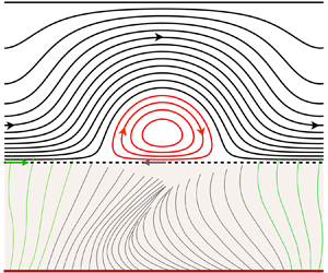
  $\omega =2{\rm \pi} f$. (b) Flow structure within the mucus layer for viscoelastic mucus (where BC means boundary condition). DNS with the code Basilisk, using the Oldroyd-B model (2.2) and periodic boundary conditions: $\lambda ={52}\ {\rm ms}$, $\beta =0.1$, $h_0^\star = {10}\ {\mathrm {\mu }}{\rm m}$, $\varLambda ^\star ={20}\ {\mathrm {\mu }}{\rm m}$, $a^\star =1.6\ {\mathrm {\mu }}{\rm m}$, $\phi ^\star =0$, $f^\star ={10}\ {\rm Hz}$, $t^\star \omega ^\star =9{\rm \pi}$. Streamlines in the laboratory reference frame.
Smith, Gaffney & Blake (Reference Smith, Gaffney and Blake2007) developed a three-layer model, where a thin traction layer was introduced between the PCL and mucus to account for the protrusion of cilia tips into the mucus layer (Fulford & Blake Reference Fulford and Blake1986). Mucus viscoelasticity was modelled via the linear Maxwell model, introducing the relaxation time  $\lambda$. The authors reported a significant and non-monotonic variation of the net mucus flow rate with increasing $\lambda$. Owing to the use of the linear Maxwell model, the observed viscoelastic effect stems entirely from the traction layer. As we will show, viscoelastic corrections in the force-free mucus layer can enter the problem only at $O(\textit {De}^2)$, where $\textit {De}$ denotes the Deborah number $\textit {De}=\lambda \omega ^\star$, based on the angular frequency $\omega ^\star =2{\rm \pi} f^\star$. We go beyond this limitation by accounting for nonlinearity in the constitutive model, allowing us to uncover the role of viscoelasticity within the mucus layer itself, where an intricate flow pattern of counter-rotating vortices develops (figure 1b).
Sedaghat et al. (Reference Sedaghat, Shahmardan, Norouzi and Heydari2016) used the immersed boundary method (IBM) to simulate arrays of cilia beating within a layer of airway surface liquid (representing mucus and PCL). Viscoelasticity was described with the Oldroyd-B model, introducing the viscosity ratio  $\beta =\mu _{s}/(\mu _{s}+\mu _{p})$, where $\mu _{s}$ and $\mu _{p}$ denote the solvent and polymer viscosities. However, the authors used cilia density 0.1 cilia per $\mathrm {\mu } \mathrm {m}^2$, which is significantly lower than typical physiological values, i.e. 5–8 cilia per $\mathrm {\mu }\mathrm {m}^2$ (Bottier et al. Reference Bottier2017b). It was not clear from this study whether viscoelasticity helps or hinders MCC in real mucus.
In the current study, we analyse MCC via an inertialess continuum hydrodynamic model sketched in figure 1(a). We focus only on the mucus layer of height  $h_0^\star$, and model momentum transfer from the beating cilia via an experimentally validated moving-carpet Navier-slip boundary condition applied at $y=0$ (Bottier et al. Reference Bottier2017b,Reference Bottier, Peña Fernández, Pelle, Isabey, Louis, Grotberg and Filochea). This boundary condition introduces a tangential wall velocity $u_{w}(x,t)$ that mimics the metachronal wave. Mucus viscoelasticity is described with the Oldroyd-B model. Following Vasquez et al. (Reference Vasquez, Jin, Palmer, Hill and Forest2016), we fit the model parameters $\lambda$ and $\beta$ to experimental mucus data for the storage and loss moduli $G'$ and $G''$ (Hill et al. Reference Hill2014).
We solve our continuum model via two approaches. First, we perform direct numerical simulations (DNS) based on the full governing equations via the finite-volume solver Basilisk (Popinet & collaborators Reference Popinet2013–2020). Second, we derive analytical solutions for the stream function within the mucus film, based on asymptotic expansion in two different limits: (1) the weakly viscoelastic limit ( $\textit {De}\ll 1$), and (2) the limit of small cilia beat amplitude ( $a\ll 1$). The low-amplitude expansion is inspired by Lauga (Reference Lauga2007), who used this approach to investigate the effect of mucus viscoelasticity on the propulsion of microorganisms modelled as swimming sheets. As discussed in Lauga (Reference Lauga2020), that problem is in some ways equivalent to the mucociliary transport problem considered here. However, there is one important difference. The discrete nature of the cilia, which are packed with some finite density, implies the existence of slip between the mucus and the imaginary envelope of the cilia tips. This effect is accounted for in the moving-carpet Navier boundary condition used in the current paper, where we have set the slip length $\phi$ based on an empirical relation (Bottier et al. Reference Bottier, Peña Fernández, Pelle, Isabey, Louis, Grotberg and Filoche2017a), linking $\phi$ to the cilia density. Accounting for slip represents an extension of the low-amplitude analytical solution of Lauga (Reference Lauga2007), and we find that this effect is significant in the case of MCC. In contrast to the work of Man & Lauga (Reference Man and Lauga2015), who investigated the effect of wall slip on the propulsion of sheet-like microorganisms swimming in a Newtonian fluid, slip affects our problem only in the presence of viscoelasticity. This is because of the stress-free boundary condition imposed at the free surface, which implies zero average shear within the mucus layer in the Newtonian limit.
In terms of physical insight, we find that mucus elasticity reduces MCC significantly relative to the Newtonian limit, causing a drop in mucus flow rate that increases with increasing  $\textit {De}$, decreasing $a$, and decreasing slip-length $\phi$. In the case of diseased mucus (characteristic of CF), we find a 30 % reduction of MCC in the physiological frequency range $f^\star \sim 10$ Hz. By contrast, Vasquez et al. (Reference Vasquez, Jin, Palmer, Hill and Forest2016), who also applied a continuum approach but assumed a spatially invariant (temporally asymmetric) wall velocity $u_{w}(t)$, concluded that the mucus flow rate is insensitive to mucus rheology. It turns out that our account of the metachronal cilia wave via $u_{w}(x,t)$ is necessary for capturing the effect of viscoelasticity on MCC. Interestingly, a flow rate reduction also occurs in the limit of a zero-mean wall velocity $\bar {u}_{w}=\int _0^\varLambda u_{w}\,{{\rm d}\kern0.7pt x}=\int _0^{1/f} u_{w}\,{\rm d}t=0$. In that case, viscoelasticity produces a net negative flow rate, i.e. in the direction of the metachronal wave, as a result of memory effects. This result contrasts with Stokes’ second problem for viscoelastic liquids (Mitran et al. Reference Mitran, Forest, Yao, Lindley and Hill2008; Ortín Reference Ortín2020), where $u_{w}=u_{w}(t)$ is spatially invariant and the net flow rate is zero, and it further underlines the importance of the metachronal wave in MCC. Past studies have shown that a change in the waveform underlying the swimming motion of sheet-like microorganisms (Riley & Lauga Reference Riley and Lauga2015) or the geometry of the swimmer itself (Angeles et al. Reference Angeles, Godínez, Puente-Velazquez, Mendez-Rojano, Lauga and Zenit2021) can switch the effect of viscoelasticity from hindering to enhancing propulsion.
Although we focus mainly on the role of viscoelasticity by using the Oldroyd-B model, we have also checked the additional effect of shear-thinning, another known non-Newtonian property of mucus (Jory et al. Reference Jory, Donnarumma, Blanc, Bellouma, Fort, Vachier, Casanellas, Bourdin and Massiera2022). For this, we have employed the Giesekus model, which accounts accurately for both viscoelasticity and shear-thinning properties of mucus (Vasquez et al. Reference Vasquez, Jin, Palmer, Hill and Forest2016; Sedaghat et al. Reference Sedaghat, Farnoud, Schmid and Abouali2022). We find that neither our low-amplitude prediction nor our weakly viscoelastic prediction is affected significantly by shear-thinning. This is due to the nature of the associated nonlinear terms in the Giesekus model, which are quadratic in the stresses and scaled by the Deborah number. As a result, shear-thinning is weak at small amplitudes and subordinate to viscoelasticity. We find that this leads to a qualitatively different MCC response versus a generalized Newtonian description of mucus via the Carreau model (Chatelin et al. Reference Chatelin, Anne-Archard, Murris-Espin, Thiriet and Poncet2017).
Our paper is structured as follows. In § 2, we introduce the governing equations constituting our mathematical model of MCC. Next, in § 3, we quantify the viscoelastic properties of the different types of mucus considered in our computations, as well as relevant kinematic parameters linked to MCC. Section 4 details the methods employed. In § 4.1, we derive analytical solutions for the mucus flow rate based on asymptotic expansion in different limits. In § 4.2, we describe the solver employed for our DNS. Results are presented in § 5, where we first focus on characterizing the effect of viscoelasticity on the mucus flow rate (§ 5.1) by comparing with the Newtonian limit. Then, in § 5.2, we discuss the additional effect of shear-thinning via calculations based on the (multi-mode) Giesekus model. Conclusions are drawn in § 6, and the paper is completed by Appendices A and B, where we have written out several expressions intervening in the analytical solutions derived in § 4.1.
2. Mathematical description
We consider a viscoelastic mucus layer of constant height  $h_0^\star$ on the interval $y^\star =0$ to $y^\star =h_0^\star$, as sketched in figure 1(a). The mucus rheology is represented via the Oldroyd-B model, with solvent and polymeric viscosities $\mu _{s}$ and $\mu _{p}$, and relaxation time $\lambda$. Both the Reynolds number ${\textit {Re}}=\rho \,h_0^{\star 2}\omega ^\star /\mu _{s}\sim 10^{-3}$ and the capillary number $\textit {Ca}=\mu _{s}h_0^\star \omega ^\star /\sigma \sim 10^{-3}$, where $\rho$ and $\sigma$ denote the liquid mass density and surface tension, are small, thus we assume inertialess flow and a flat surface of the mucus layer (Smith et al. Reference Smith, Gaffney and Blake2007). In this limit, the flow is governed by the (dimensionless) continuity and Stokes equations with additional polymeric viscous stresses $\tau _{ij}$:
 \begin{gather} {\partial_{x}u} + {\partial_{y}v} = 0, \end{gather}
 \begin{gather}0 ={-}{\partial_{x}p}+ \left( {\partial_{xx}u} + {\partial_{yy}u} \right)+{\partial_{x}\tau}_{xx} + {\partial_{y}\tau}_{xy}, \end{gather}
 \begin{gather}0 ={-}{\partial_{y}p}+ \left( {\partial_{xx}v} + {\partial_{yy}v} \right)+{\partial_{x}\tau}_{xy} + {\partial_{y}\tau}_{yy}, \end{gather}
where we have scaled lengths with  $\mathcal {L}=h_0^\star$, velocities with $\mathcal {U}=h_0^\star \,\omega ^\star$, and $\tau _{ij}$ as well as pressure $p$ with $\mathcal {P}=\mu _{s}\mathcal {U}/\mathcal {L}$, using the angular frequency of the cilia beat cycle $\omega ^\star$. The components of the polymeric stress tensor $\tau _{ij}$ are governed by the upper-convected Maxwell model:
 \begin{gather} \tau_{xx} + \textit{De} \left[{\partial_{t}\tau}_{xx} + u\,{\partial_{x}\tau}_{xx} + v\,{\partial_{y}\tau}_{xx} - 2\tau_{xx}\,{\partial_{x}u} - 2\tau_{xy}\,{\partial_{y}u}\right]= 2\,\frac{1-\beta}{\beta}\,{\partial_{x}u}, \end{gather}
 \begin{gather}\tau_{xy} + \textit{De} \left[{\partial_{t}\tau}_{xy} + u\,{\partial_{x}\tau}_{xy} + v\,{\partial_{y}\tau}_{xy} - \tau_{xx}\,{\partial_{x}v} - \tau_{yy}\,{\partial_{y}u}\right]=\frac{1-\beta}{\beta}\left({\partial_{y}u} + {\partial_{x}v}\right), \end{gather}
 \begin{gather}\tau_{yy} + \textit{De} \left[{\partial_{t}\tau}_{yy} + u\,{\partial_{x}\tau}_{yy} + v\,{\partial_{y}\tau}_{yy} - 2\tau_{xy}\,{\partial_{x}v} - 2\tau_{yy}\,{\partial_{y}v}\right]=2\,\frac{1-\beta}{\beta}\,{\partial_{y}v}, \end{gather}
where we have scaled time with  $\mathcal {T}=1/\omega ^\star$, yielding the Deborah number $\textit {De}=\lambda \omega ^\star$ and the viscosity ratio $\beta =\mu _{s}/(\mu _{s} + \mu _{p})$. The system is closed with the following boundary conditions. At the film surface, $y=1$, we impose
 \begin{gather} {\partial_{y}u} + \tau_{xy} = 0, \end{gather}
 \begin{gather}v = 0, \end{gather}
where we have assumed impermeability and neglected viscous stresses in the gas above the mucus layer. At the bottom boundary,  $y=0$, we impose the Navier-slip boundary condition introduced by Bottier et al. (Reference Bottier, Peña Fernández, Pelle, Isabey, Louis, Grotberg and Filoche2017a) for modelling momentum transfer from the beating cilia:
 \begin{equation} u-\phi\,\partial_y u=u_{w}(x,t),\quad v=0, \end{equation}
where  $\phi$ denotes the (dimensionless) slip length. Here, the cilia kinematics is represented via the wave function
 \begin{equation} u_{w}(x,t)=a\cos(kx+ t)+\zeta\tfrac{1}{2}a^2 k \left[1-\cos\{2(kx+t)\}\right], \end{equation}
introducing the cilia beat amplitude  $a$, and the metachronal wavenumber $k=2{\rm \pi} /\varLambda$, where the dimensionless wavelength $\varLambda =\varLambda ^\star /h_0^\star$, due to the scaling chosen, sets the aspect ratio of our geometry. Without loss of generality, we have phase shifted $u_{w}(x,t)$ by ${\rm \pi} /2$ with respect to the classical formulation of Bottier et al. (Reference Bottier, Peña Fernández, Pelle, Isabey, Louis, Grotberg and Filoche2017a). The parameter $\zeta$ is a binary parameter that takes values $\zeta =0$ and $1$, and can be used to deactivate the second and third right-hand-side terms in (2.4b). In that limit, i.e. $\zeta =0$, the phase average $\bar {u}_{w}$ is zero, which, in the case of a Newtonian fluid, leads to a symmetrical cellular flow pattern (e.g. figure 2a). This reference case is convenient for illustrating the signature of viscoelasticity, which tends to break the symmetry of the flow field (e.g. figure 6e). The moving-carpet boundary condition written in (2.4) has been validated versus particle image velocimetry measurements in the vicinity of live beating cilia (Bottier et al. Reference Bottier2017b).

Figure 2. Flow structure within the mucus film. Newtonian limit:  $\textit {De}=0$, $\varLambda ^\star ={20}\ {\mathrm {\mu }}{\rm m}$. (a,b) Streamlines for two forms of the wave function (2.4b): $a^\star ={1.6}\ {\mathrm {\mu }}{\rm m}$, $\phi ^\star =0$, $t={\rm \pi}$. Solid red line indicates analytical solution (4.3a); dashed blue line indicates DNS using $\Delta x=1/64$; dotted black line (almost perfectly overlapping solid red line) indicates DNS using $\Delta x=1/128$. Here: (a) $\zeta =0$, cellular flow pattern; (b) $\zeta =1$, meandering flow; (c) estimation of maximum film surface deflection according to (4.5) for different values of the slip length $\phi ^\star$, with $a^{\star }={5}\ {\mathrm {\mu }}{\rm m}$, $\textit {Ca}=1\times 10^{-3}$. Dashed line indicates $\phi ^\star =0$; dotted line indicates $\phi ^\star ={2}\ {\mathrm {\mu }}{\rm m}$; dot-dashed line indicates $\phi ^\star ={5}\ {\mathrm {\mu }}{\rm m}$; solid line indicates $\phi ^\star ={10}\ {\mathrm {\mu }}{\rm m}$.
As a key observable in our study, we evaluate the net mucus flow rate
 \begin{equation} q=\int_0^1 u\,{{\rm d}y}, \end{equation}
which is spatially invariant due to continuity and the flat-surface assumption, i.e.  $\partial _xq=-\partial _th=0$, and time-invariant due to the wave nature of $u_{w}$ (see (2.4b)). In the Newtonian limit (subscript ${N}$), the governing equations become linear, thus the flow field is a simple superposition of the solutions associated with the three terms in the wave function (2.4b). Because the phase average of the two harmonic terms is zero, only the constant term contributes to the net flow, yielding
 \begin{equation} q_{N}=\zeta q_{ref},\quad\text{with}\ q_{ref}\equiv\tfrac{1}{2}a^2k, \end{equation}
which corresponds to a plug flow with wall velocity  $u_{w}=\zeta a^2 k/2$. Throughout the paper, we will use $q_{N}$ (and $q_{ref}$) as a reference value to quantify the effect of viscoelasticity.
3. MCC scenarios: mucus types and cilia parameters
Experimentally, the mechanical response of viscoelastic mucus is quantified via the complex modulus  $G=G'+{\rm i}G''$, containing the storage and loss moduli $G'$ and $G''$, which are related to the parameters of the Oldroyd-B model according to Siginer (Reference Siginer2014):
 \begin{equation} \frac{G'}{\mu_{s}\omega^\star}=\frac{1-\beta}{\beta}\,\frac{\lambda \omega^\star}{1+(\lambda\omega^\star)^2}, \quad \frac{G''}{\mu_{s}\omega^\star}=1 + \frac{1-\beta}{\beta [1+(\lambda\omega^\star)^2]}. \end{equation}
We focus on four types of mucus corresponding to human bronchial epithelial (HBE) cultures with varying mucin concentration (Hill et al. Reference Hill2014), ranging from healthy patients ( $2~{\rm wt}\%$) to patients diagnosed with CF or COPD (5 wt%). The properties of these mucus types are provided in table 1. We have assumed water as the solvent phase, i.e. $\mu _{s}={1}\ {\rm mPa}\ {\rm s}$, and fitted $\beta$ and $\lambda$ to experimental values of $G'$ and $G''$ (Hill et al. Reference Hill2014) at a representative cilia beat frequency $f^\star \sim 10$ Hz. Accounting for the frequency dependence of $\beta$ and $\lambda$ does not change our results significantly (as shown in figure 3a).
Table 1. Human bronchial epithelial (HBE) mucus types and cilia beat amplitude  $a^\star$ used in our simulations. Measurement data for $G'$ and $G''$, ranging from healthy to diseased mucus, are taken at $f^\star \sim 10\ {\rm Hz}$ from Hill et al. (Reference Hill2014). Oldroyd-B model parameters $\lambda$ and $\beta$ were fitted via (3.1a,b), assuming $\mu _{s}={1}\ {\rm mPa}\ {\rm s}$.


Figure 3. Features of the flow within a viscoelastic mucus layer: HBE-5 wt% mucus,  $h_0^\star ={10}\ {\mathrm {\mu }}\textrm {m}$, $\varLambda ^\star ={20}\ {\mathrm {\mu }}\textrm {m}$, $a^\star ={1.6}\ {\mathrm {\mu }}\textrm {m}$, $\phi ^\star ={10}\ {\mathrm {\mu }}\textrm {m}$. (a) Average mucus velocity $\bar {u}^\star =q^\star /h_0^\star$. The solid line indicates the Newtonian limit; the dot-dashed line is based on (4.9) with $\lambda =52\ \textrm {ms}$, $\beta =0.1$; the dashed line is based on (4.9) with frequency-dependent $\lambda$ and $\beta$ according to $G'$ and $G''$ data in Hill et al. (Reference Hill2014). Symbols indicate our DNS: circles, $\Delta x=1/32$; squares, $\Delta x=1/64$; plus signs, $\Delta x=1/128$. (b) Streamlines and contours of the trace $\mathrm {tr}(\boldsymbol{\mathsf{C}})$ of the conformation tensor $\boldsymbol{\mathsf{C}}=\textit {De}\,\boldsymbol {\tau }_{ij}+\boldsymbol{\mathsf{I}}$ based on the Oldroyd-B model: $\lambda ={52}\ \textrm {ms}$, $\beta =0.1$, $f^\star ={19}\ \textrm {Hz}$, $t=9{\rm \pi}$.
In the case of CF, the PCL layer is depleted in favour of the mucus layer, which can reduce considerably the mucus velocity imparted by the cilia (Guo & Kanso Reference Guo and Kanso2017). We account for this by adjusting the beat amplitude  $a$ in terms of the mucin concentration (see table 1), by interpolating between experiments for healthy mucus (Bottier et al. Reference Bottier2017b), $a^\star ={5}\ {\mathrm {\mu }}{\rm m}$, and diseased mucus (Bottier et al. Reference Bottier2022), $a^\star ={1.6}\ {\mathrm {\mu }}{\rm m}$.
Bottier et al. (Reference Bottier2017b) established experimentally a relation between the cilia density and the slip length  $\phi ^\star$. We use 86 % cilia density in our simulations, which is representative of the patient data reported in that reference, yielding slip length $\phi ^\star ={10}\ {\mathrm {\mu }}{\rm m}$.
4. Methods
4.1. Analytical solutions via asymptotic expansion
We obtain analytical solutions for our boundary value problem (2.1)–(2.4) in two different limits: (i) small Deborah number ( $\textit {De} \ll 1$), and (ii) small cilia beat amplitude ( $a\ll 1$). For this, we introduce the stream function $\varPsi$,
 \begin{equation} \partial_y\varPsi=u,\quad-\partial_x\varPsi=v, \end{equation}
to which we apply a regular perturbation expansion
 \begin{equation} \varPsi(x,y,t)=\varPsi_0(x,y,t)+{\epsilon}\,\varPsi_1(x,y,t)+{\epsilon}^2\,\varPsi_2(x,y,t), \end{equation}
where the small parameter  ${\epsilon }$ is either $\textit {De}$ or $a$, depending on the expansion considered. Then, introducing (4.2) into (2.1)–(2.4) and truncating appropriately, we may obtain $\varPsi _i$ order by order. We point out that $\varPsi _0$ is the solution of the biharmonic equation, obtained by eliminating pressure from the truncated forms of (2.1b) and (2.1c) via cross-differentiation.
In the weakly viscoelastic limit, we expand in terms of  ${\epsilon }=\textit {De}$ and obtain at $O(\textit {De}^2)$,
 \begin{gather}
\varPsi_0(x,y,t)=\left[
(A_1 + B_1ky)\,{\rm e}^{ky} + (C_1 +
D_1ky)\,{\rm e}^{{-}ky} \right]\cos(kx+t) + \zeta
A_2y \nonumber\\ + \zeta\left[ (A_3 +
2B_3ky)\,{\rm e}^{2ky} + (C_3 +
2D_3ky)\,{\rm e}^{{-}2ky} \right]\cos\{2(kx+t)\},
\end{gather}
\begin{gather}
\varPsi_0(x,y,t)=\left[
(A_1 + B_1ky)\,{\rm e}^{ky} + (C_1 +
D_1ky)\,{\rm e}^{{-}ky} \right]\cos(kx+t) + \zeta
A_2y \nonumber\\ + \zeta\left[ (A_3 +
2B_3ky)\,{\rm e}^{2ky} + (C_3 +
2D_3ky)\,{\rm e}^{{-}2ky} \right]\cos\{2(kx+t)\},
\end{gather}
 \begin{gather} \varPsi_1(x,y,t)=0, \end{gather}
 \begin{gather}\varPsi_2(x,y,t)=\varPsi_H(x,y,t)+\varPsi_P(x,y,t), \end{gather}
where  $A_i$, $B_i$, $C_i$ and $D_i$ are integration constants, and $\varPsi _H(x,y,t)$ and $\varPsi _P(x,y,t)$ denote homogeneous and particular solutions, which are all written out in Appendix A, and in a supplementary Mathematica notebook available at https://doi.org/10.1017/jfm.2023.682. A simple relation for the flow rate $q=\varPsi |_{y=1}-\varPsi |_{y=0}$ can be obtained by considering (4.3) in the limit $\zeta =0$:
 \begin{equation} \left.{\frac{q}{q_{ref}}}\right|_{\zeta=0}={-}(1-\beta)\,\textit{De}^2\,\frac{S^2+6k\phi SC}{(S+2k\phi C)^2}+O(\textit{De}^3), \end{equation}
where  $S=\sinh (2k)-2k$ and $C=\cosh (2k)-1$. We see that viscoelasticity enters at $O(\textit {De}^2)$, and constitutes a negative flow rate contribution. The full form of ${q}/q_{ref}$ for $\zeta =1$ is too long to be written here. Instead, we provide it in the supplementary Mathematica notebook. In the Newtonian limit ( $\textit {De}=0$), (4.2) reduces to $\varPsi _0$, which we have plotted in figures 2(a) and 2(b) for the reduced ( $\zeta =0$) and full ( $\zeta =1$) forms of (2.4b), respectively. In the former case, the flow pattern is cellular (figure 2a), and, in the latter, it is meandering (figure 2b).
The leading-order solution  $\varPsi _0$ can also be used to estimate the deflection of the liquid–gas interface $h'$:
$h'$:
 \begin{equation} h' = \textit{Ca}\left\{\frac{4a\cosh(k)}{S+2k\phi C}-\frac{4a^2k\zeta\cosh(2k)\cos(kx+t)}{S'+2k'\phi C'}\right\}\sin(kx+t), \end{equation}
where  $S'=\sinh (2k')-2k'$ and $C'=\cosh (2k')-1$, introducing $k'=2k$. This relation is obtained by balancing the normal stress acting at our flat liquid–gas interface, $y=1$, with the capillary pressure jump of a deformable film surface, $h=1+h'$:
 \begin{equation} p-2\,{\partial_{y}v}- \tau_{yy}={-}\textit{Ca}^{{-}1}\,\partial_{xx}h, \end{equation}
where we have neglected the gas stresses, then truncating at  ${O}(\textit {De}^0)$, and substituting the leading-order solutions for $\varPsi$ (4.3a) and for $p$ (4.7) into (4.6). The leading-order pressure $p_0$ is obtained by integrating (2.1c) in the $y$-direction and (2.1b) in the $x$-direction, after having applied (4.2), truncated, and substituted (4.3a):
 \begin{equation} p_0 = 2{\rm e}^{{-}2ky}\,k^2\sin(kx+t)\,\{{\rm e}^{ky}\,(D_1+B_1\,{\rm e}^{2ky})+8\zeta\cos(kx+t)\,(D_3+B_3\,{\rm e}^{4ky})\}, \end{equation}
where, without loss of generality, we have assumed  $p_0(x=0,y=0,t)=0$.
Figure 2(c) represents the maximum displacement  $h'_{max}$ obtained from (4.5) versus the dimensional film height $h_0^\star$, demonstrating that our flat-surface assumption ( $\partial _{x}h=\partial _{xx}h=0$) is valid within the physiological film thickness range $h_0^\star =5\unicode{x2013}20\ {\mathrm {\mu }}{\rm m}$, for the largest cilia beat amplitude considered, i.e. $a^\star =5\ {\mathrm {\mu }}{\rm m}$.
In the low-amplitude limit, we expand (4.2) in terms of  ${\epsilon }=a$ and seek a solution for the time-averaged stream function $\bar {\varPsi }(y)$. For $\zeta =1$, we obtain
 \begin{equation} \left.\begin{gathered} \bar{\varPsi}(y)=a^2\,\bar{\varPsi}_2(y)+O(a^3),\\ \bar{\varPsi}_2(y)= \left(I_0 + I_1 y + I_2 y^2\right){\rm e}^{2ky} + \left(J_0 + J_1 y + J_2 y^2\right){\rm e}^{{-}2ky} + K_1 y + K_2 y^2, \end{gathered}\right\} \end{equation}
where the constants  $I_i$, $J_i$ and $K_i$ are given in Appendix B. Based on (4.8), we obtain the normalized flow rate:
 \begin{equation} \frac{q}{q_{N}}= 1 - \frac{(1-\beta)\,\textit{De}^2\,(S^2+6\phi k S C)}{(1+\textit{De}^2)(S+2\phi k C)^2} + O(a^3). \end{equation}
In the no-slip limit  $\phi =0$, (4.9) collapses with (26) in Lauga (Reference Lauga2007), which predicts the normalized swimming speed $U/U_N$ of microorganisms represented as Taylor swimming sheets. In figure 3(a), we have plotted the average mucus velocity $\bar {u}^\star =q^\star /h_0^\star$ based on (4.9) versus the cilia beat frequency $f^\star$. The dot-dashed and dashed red curves correspond to viscoelastic mucus, assuming constant (dot-dashed) or frequency-dependent (dashed) values of $G'$ and $G''$, based on experimental data of Hill et al. (Reference Hill2014). Comparing these curves, we may conclude that our approximation to neglect the frequency dependence of $G'$ and $G''$ is reasonable in the considered frequency range. The solid black curve in figure 3(a) corresponds to the Newtonian limit ( $\textit {De}=0$), where $q^\star$ increases linearly with $f^\star$ (Blake Reference Blake1973; Sedaghat et al. Reference Sedaghat, Shahmardan, Norouzi and Heydari2016). The exact relation underlying this curve is $q^\star =q^\star _{N}={\rm \pi} a^{\star 2} k f^\star$, which follows from (2.6) upon re-dimensionalizing with the scale $\mathcal {U}\mathcal {L}=h_0^{\star 2}\omega ^\star$.
4.2. Direct numerical simulations
We solve numerically the fully nonlinear governing equations (2.1)–(2.4) on a periodic domain using the academic code Basilisk, which employs the log-conform approach (López-Herrera, Popinet & Castrejón-Pita Reference López-Herrera, Popinet and Castrejón-Pita2019) for resolving the constitutive relations (2.2). It is a pressure-based solver, thus the Poisson equation for the pressure is solved instead of (2.1a) to enforce continuity (Popinet Reference Popinet2015), using the boundary conditions  $\partial _y p = 0$ at $y=0$ and (4.6) at $y=h$, in the limit $h=1$. The same code was used recently by Romano et al. (Reference Romano, Muradoglu, Fujioka and Grotberg2021) to investigate the effect of viscoelasticity on airway occlusion, and validated versus several relevant benchmarks. The code relies on a finite-volume spatial discretization, using the second-order upwind Bell–Colella–Glaz advection scheme (Bell, Colella & Glaz Reference Bell, Colella and Glaz1989). Time discretization is implicit for diffusion and explicit for advection terms, and the time step is adapted according to a CFL criterion. Our DNS were typically performed on a uniform quadtree grid, with grid size $\Delta x=2^{-6}=1/64$, and the time step was limited by a lower bound $\Delta t=10^{-7}$. A typical DNS run took 5–18 h on 8 CPUs to reach a fully developed state (after 3–10 periods).
In figures 2(a) and 2(b), we have included grid convergence results obtained with our DNS for the Newtonian reference case. Dashed blue curves correspond to grid size  $\Delta x=1/64$, and dotted black curves to $\Delta x=1/128$. Agreement with our analytical predictions (solid red curves) according to (4.3a) is visually perfect for the fine grid and remains excellent for the reference grid. The same conclusion can be drawn from figure 3(a), which confronts DNS using three different grids (symbols) with our low-amplitude asymptotic solution (dot-dashed curve) according to (4.9), for a viscoelastic mucus film.
Figure 3(b) represents streamlines for one of our DNS from figure 3(a). In the same plot, we have represented contours of the trace  $\mathrm {tr}(\boldsymbol{\mathsf{C}})$ of the conformation tensor $\boldsymbol{\mathsf{C}}=\textit {De}\,\boldsymbol {\tau }_{ij}+\boldsymbol{\mathsf{I}}$ based on the Oldroyd-B model, where $\boldsymbol{\mathsf{I}}$ is the identity matrix. The quantity $\mathrm {tr}(\boldsymbol{\mathsf{C}})$ allows us to gauge the polymer extension associated with our flow field. We find that the maximum value, observed near the cilia–mucus interface, is $\mathrm {tr}(\boldsymbol{\mathsf{C}})\sim 2.5$, which implies a moderate fluid element extension relative to the Newtonian limit $\mathrm {tr}(\boldsymbol{\mathsf{C}})=2$. Thus the Oldroyd-B model employed here is expected to behave well for our flow.
In our problem, the mucus viscosities  $\mu _{s}$ and $\mu _{p}$ intervene only via $\beta$. Thus the total viscosity $\mu =\mu _{s}+\mu _{p}$ can be chosen freely. For numerical convenience, we choose a low value $\mu ={1}\ \textrm {mPa}\ \textrm {s}$, allowing us to limit the viscous diffusion time scale. The log-conform approach is an effective remedy against numerical instabilities associated with large values of $\textit {De}$ (Fattal & Kupferman Reference Fattal and Kupferman2005), and we have encountered no such instabilities in our DNS. However, in our simulations of HBE-5 wt% mucus, we needed to increase $\beta$ from its target value $\beta =0.002$ to $\beta =0.1$, because of the degeneracy of the constitutive relations (2.2) in the limit $\beta \to 0$. We have checked via (4.9) that this change in $\beta$ has no appreciable effect on the MCC flow rate.
5. Results and discussion
Our main results are presented in § 5.1, where we focus solely on the effect of viscoelasticity. In § 5.2, we will discuss the additional implications of shear-thinning, which is another non-Newtonian property of mucus.
5.1. Role of viscoelasticity
We seek to quantify the effect of mucus viscoelasticity on MCC by comparing the actual flow rate  $q$ (2.5) to its Newtonian limit $q_{N}$. For this, we characterize the ratio $q/q_{N}$ versus three control parameters of our problem, i.e. $\textit {De}$, $\phi$ and $a$. We start with figure 4 by establishing the effect of the slip length $\phi$ and beat amplitude $a$, in order to assess to what extent the no-slip low-amplitude theory of Lauga (Reference Lauga2007) is applicable to the MCC problem studied here. Figure 4(a) shows predictions of $q/q_{N}$ based on our low-amplitude solution (4.9) for different slip lengths $\phi$ and representative values of $\textit {De}$ and $\beta$. First, we see that viscoelasticity can greatly reduce the MCC flow rate ( $q/q_{N}<1$). Second, this effect is much larger in the no-slip limit (long dashes) than for realistic values of $\phi$ (solid curve). Third, the no-slip limit cannot represent the $q/q_{N}$ variation in terms of the film height $h_0^\star$.

Figure 4. Effect of slip length  $\phi$ and CBA $a$ on the MCC flow rate of viscoelastic mucus: $\varLambda ^\star ={20}\ {\mathrm {\mu }}\textrm {m}$. (a) Effect of slip-length: $\textit {De}=3$, $\beta =0.1$. Low-amplitude prediction (4.9). Dashed line indicates $\phi ^\star =0$; dotted line indicates $\phi ^\star ={2}\ {\mathrm {\mu }}\textrm {m}$; dot-dashed line indicates $\phi ^\star ={5}\ {\mathrm {\mu }}\textrm {m}$; solid line indicates $\phi ^\star ={10}\ {\mathrm {\mu }}\textrm {m}$. (b) Effect of CBA: $\phi =0$, $\beta =0.5$, $h_0^\star ={10}\ {\mathrm {\mu }}\textrm {m}$. Dotted lines based on low- $\textit {De}$ prediction (4.3); dashed line indicates (4.9). Symbols indicate DNS: circles, $a^\star ={1.6}\ {\mathrm {\mu }}\textrm {m}$; triangles, $a^\star ={3}\ {\mathrm {\mu }}\textrm {m}$; squares, $a^\star ={5}\ {\mathrm {\mu }}\textrm {m}$; diamonds, $a^\star ={8}\ {\mathrm {\mu }}\textrm {m}$.
Figure 4(b) represents the effect of the cilia beat amplitude (CBA)  $a$ in the no-slip limit $\phi =0$ via DNS data (symbols). We see that $q/q_{N}$ becomes very small at the lowest CBA (circles, $a^\star ={1.6}\ {\mathrm {\mu }}\textrm {m}$), which corresponds to CF conditions. The low-amplitude analytical prediction (4.9) (black dashed curve) is able to capture accurately this scenario versus the DNS (open circles). By contrast, a significant discrepancy is observed for the CBA corresponding to healthy conditions (diamonds, $a^\star ={8}\ {\mathrm {\mu }}\textrm {m}$). Thus the low-amplitude asymptotic expansion is not applicable in the entire physiological range of MCC, owing to potentially large values of CBA. The dotted curves in figure 4(b) represent our low- $\textit {De}$ solution (4.3). These show good agreement with the DNS for low values of $\textit {De}$, but cannot predict the levelling off of $q/q_{N}$ with increasing $\textit {De}$. The deviation from the DNS data sets in at lower values of $\textit {De}$ the larger $a$ becomes.
We now turn to the MCC scenarios characterized in table 1. If not mentioned otherwise, we use  $h_0^\star ={10}\ {\mathrm {\mu }}\textrm {m}$, $\phi ^\star ={10}\ {\mathrm {\mu }}\textrm {m}$ and $\varLambda ^\star ={20}\ {\mathrm {\mu }}\textrm {m}$. Figures 5(a) and 5(b) represent DNS and analytical predictions of $q/q_{N}$ for the four considered mucus types versus the Deborah number $\textit {De}$ and versus the cilia beat frequency $f^{\star }$, respectively. In the case of healthy mucus (HBE-2 wt%, blue circles), which is characterized by a rather small relaxation time $\lambda$, viscoelasticity reduces MCC only slightly ( $q/q_N\sim 0.995- 0.98$) within the physiological frequency range $f^\star =5- {20}\ \textrm {Hz}$ (green shaded region in figure 5b). This contrasts with the very significant reduction in the swimming speed $U$ of non-ciliated microorganisms (dot-dashed blue curve), which operate at much greater frequencies ( $\,f^\star > {80}\ \textrm {Hz}$, pink shaded region) and do not experience slip, as predicted by the theory of Lauga (Reference Lauga2007). We point out, however, that particular types of swimming motions and swimmer geometries can lead to a viscoelasticity-induced increase of the swimming speed (Riley & Lauga Reference Riley and Lauga2015; Angeles et al. Reference Angeles, Godínez, Puente-Velazquez, Mendez-Rojano, Lauga and Zenit2021).

Figure 5. Viscoelasticity-induced flow rate reduction for mucus types from table 1:  $\phi ^\star ={10}\ {\mathrm {\mu }}\textrm {m}$, $h_0^\star ={10}\ {\mathrm {\mu }}\textrm {m}$, $\varLambda ^\star ={20}\ {\mathrm {\mu }}\textrm {m}$. Symbols indicate DNS: blue circles, HBE-2 wt%; cyan triangles, HBE-3 wt%; magenta squares, HBE-4 wt%; red diamonds, HBE-5 wt%. Dotted lines based on (4.3); dashed lines indicate (4.9). (a) Versus Deborah number $\textit {De}=\lambda \omega ^\star$. (b) Versus cilia beat frequency $f^{\star }$. Dot-dashed lines (right ordinate) indicate normalized swimming speed $U/U_{N}$ of microorganisms according to Lauga (Reference Lauga2007). Green/pink shaded regions mark the frequency ranges for MCC and microorganism propulsion, respectively.
In the case of mucus corresponding to CF conditions (HBE-5 wt%, red diamonds in figure 5), which displays a much greater relaxation time  $\lambda$, the MCC flow rate drops by as much as 30 % versus the Newtonian limit. This is due mainly to the reduced CBA associated with CF conditions. Dashed curves in figure 5(b) represent our low-amplitude analytical prediction (4.9). Upon comparing these with our DNS data (symbols), we may conclude that the analytical prediction captures accurately $q/q_{N}$ in the MCC frequency range for the healthy mucus (circles) and for the most unhealthy mucus (diamonds). However, significant deviations are observed for the intermediate mucus types (triangles and squares).
Next, we turn to the mechanism underlying the viscoelasticity-induced flow rate drop observed in figure 5. To this end, it is useful to reduce the problem to a simpler version by setting  $\phi =0$ and $\zeta =0$ in (2.4b), which leads to $\bar {u}_{w}=0$. We have shown in figure 2(a) that the corresponding flow pattern in the Newtonian limit is cellular and symmetrical, and consequently, $q=q_{N}=0$. Adding viscoelasticity, which we now know to affect the flow rate $q$, will thus cause a topological change in the flow field.
Figure 6(a) demonstrates via DNS data (symbols) that a similar flow rate reduction is observed for the reduced form of the wave function (2.4b), i.e.  $\zeta =0$ (squares), as compared to the full form, i.e. $\zeta =1$ (circles). Further, the mucus flow rate $q$ becomes negative for $\zeta =0$, and this effect holds at arbitrarily low $\textit {De}$. The effect is captured by our low- $\textit {De}$ solution (4.4), which is represented via a dotted blue curve in figure 6(a). Figure 6(b) shows how viscoelasticity modifies the flow field in this limit, by plotting $\varPsi _0$ and $\varPsi _2$ according to (4.3). We see that the $O(\textit {De}^2)$ correction (dashed lines) causes a net flow to the left, which distorts the $O(\textit {De}^0)$ cellular flow pattern (solid lines) when superimposed on the latter. Figures 6(c)–6(f) display the total flow field obtained from DNS for the points marked by filled symbols in figure 6(a). We see that viscoelasticity causes a negative meander (as opposed to the positive meander observed in figures 1(b) and 2(b)), which winds between the counter-rotating vortices and increases in thickness as $\textit {De}$ is increased (from figures 6c–f). This negative meander transports mucus in the direction of the metachronal wave, i.e. in the negative $x$-direction, and thus the wrong direction from the point of view of MCC. It is associated with the $\cos (kx+t)$ term in the wall velocity $u_{w}$ (see (2.4b)), and, in the full MCC problem ( $\zeta =1$), it opposes the positive flow induced by the term with the form $a^2k/2$.

Figure 6. Change in flow topology within a viscoelastic mucus film under an increase of the cilia beat frequency: HBE-5 wt% (see table 1),  $\phi =0$, $a^\star ={1.6}\ {\mathrm {\mu }}\textrm {m}$, $\varLambda ^\star ={20}\ {\mathrm {\mu }}\textrm {m}$, $h_0^\star ={10}\ {\mathrm {\mu }}\textrm {m}$. (a) Normalized flow rate for two forms of (2.4b). Circles indicate DNS for $\zeta =1$; squares indicate DNS for $\zeta =0$; dotted blue curves indicate low- $\textit {De}$ solutions based on (4.3). (b) Plots of $\varPsi _0$ (solid) and $\varPsi _2$ (dashed) according to (4.3): $\textit {De}=0.1$. (c–f) Streamlines from DNS corresponding to filled squares in (a), showing the emergence of a negative meander (black lines) sandwiched between clockwise (red lines) and anticlockwise (blue lines) vortices, as $\textit {De}$ is increased: (c) $\textit {De}=0.1$, (d) $\textit {De}=0.5$, (e) $\textit {De}=1$, and (f) $\textit {De}=2$.
To unravel what causes the negative meander observed in figure 6, we analyse the different terms in the  $x$-momentum equation (2.1b) evaluated at $y=0$, based on our low- $\textit {De}$ solution (4.3) in the limit $\zeta =\phi =0$. Profiles of these terms, which we denote $\varXi _i$, are plotted in figure 7(a), and their phase averages $\bar {\varXi }_i$ are given in the caption. The dashed blue curve represents the contribution of the solvent stresses $\varXi _1=\partial _{xx}u+\partial _{yy}u$, which allows one to gauge the degree of symmetry of the flow field. This curve is shifted towards positive values compared to the Newtonian limit $\varXi _0={\varXi _1}|_{\textit {De}=0}=\partial _{xx}u^{(0)}+\partial _{yy}u^{(0)}$ (solid blue curve, $\bar {\varXi }_0=0$), i.e. its phase average is non-zero ( $\bar {\varXi }_1=0.18$), indicating a viscoelasticity-induced loss of symmetry. This is caused mainly by the contribution of the tangential polymeric stress $\varXi _3=\partial _y\tau _{yx}$ (dot-dashed red curve, $\bar {\varXi }_3=-0.16$), the contributions of the normal stress $\varXi _2=\partial _y\tau _{yx}$ (dotted red curve, $\bar {\varXi }_3=0.004$) and the pressure $\varXi _2=\partial _x p$ (dot-dot-dashed black curve, $\bar {\varXi }_2=0.024$) being weaker.

Figure 7. Mechanism underlying the negative meander in figure 6:  $\phi =0$, $\zeta =0$, $h_0^\star ={10}\ {\mathrm {\mu }}\textrm {m}$, $\varLambda ^\star ={20}\ {\mathrm {\mu }}\textrm {m}$, $\textit {De}=0.1$. (a) Profiles of terms $\varXi _i$ in the $x$-momentum equation (2.1b) evaluated at $y=0$, based on our low- $\textit {De}$ solution (4.3), and their phase averages $\bar {\varXi }_i$. Dashed line indicates $\varXi _1=\partial _{xx}u+\partial _{yy}u$, $\bar {\varXi }_1=0.18$; solid line indicates $\varXi _0={\varXi _1}|_{\textit {De}=0}=\partial _{xx}u^{(0)}+\partial _{yy}u^{(0)}$, $\bar {\varXi }_0=0$; dotted line indicates $\varXi _2=\partial _x\tau _{xx}$, $\bar {\varXi }_2=0.004$; dot-dashed line indicates $\varXi _3=\partial _y\tau _{yx}$, $\bar {\varXi }_3=-0.16$; dot-dot-dashed line indicates $\varXi _4=\partial _x p$, $\bar {\varXi }_4=0.024$ (long dashes). (b) Polymeric wall shear stress $\tau _{xy}^{VE}$ according to (5.1). Solid line indicates $\tau _{yx}^{VE}$, $\bar {\tau }_{yx}^{VE}=0.013$ (dot-dashed); dashed line indicates $\tau ^{\textit {res}}_{yx}$, $\bar {\tau }^{\textit {res}}_{yx}=0.0003$; dotted line indicates $\tau ^{mem}_{yx}$, $\bar {\tau }^{mem}_{yx}=0.0127$.
We focus next on the tangential polymeric stress at  $y=0$:
 \begin{equation} \left.{\tau_{yx}}\right|_{y=0}=\frac{1-\beta}{\beta}\left.{\partial_yu^{(0)}}\right|_{y=0}+\underbrace{\textit{De} \left.{\tau_{yx}^{(1)}}\right|_{y=0}+\textit{De}^2 \left.{\tau_{yx}^{(2)}}\right|_{y=0}}_{\tau_{yx}^{VE}}+O(\textit{De}^3), \end{equation}
where  $\tau _{yx}^{VE}$ is the viscoelastic contribution, which we decompose formally into a memory term $\tau _{yx}^{mem}$, containing all time derivatives intervening through (2.2), and a residual term $\tau _{yx}^{\textit {res}}$, containing all other contributions:
 \begin{equation} \tau_{yx}^{VE}\equiv \tau_{yx}^{mem}+\tau_{yx}^{\textit{res}}. \end{equation}
Figure 7(b) represents profiles of  $\tau _{yx}^{VE}$ (solid black), $\tau _{yx}^{mem}$ (dotted magenta) and $\tau _{yx}^{res}$ (dashed green), and the corresponding phase averages are given in the caption. We see that $\bar {\tau }_{yx}^{VE}$ is positive (dot-dashed black line, $\bar {\tau }_{yx}^{VE}=0.013$), which corresponds to a negative tangential stress acting on the mucus, and that this non-zero phase average is due mainly to the memory term ( $\bar {\tau }_{yx}^{mem}=0.0127$). Thus it is the memory terms in the viscoelastic constitutive relations (2.2) that cause a non-symmetrical stress distribution, breaking the symmetry of the cellular flow pattern observed in the Newtonian limit. We point out that $\tau _{xy}^{mem}$ contains time derivatives stemming from (2.2a) and (2.2c), due to the nonlinear terms in the upper-convected derivative.
5.2. Additional role of shear-thinning
It has been demonstrated by Jory et al. (Reference Jory, Donnarumma, Blanc, Bellouma, Fort, Vachier, Casanellas, Bourdin and Massiera2022) that mucus also exhibits a shear-thinning behaviour over a considerable range of strain rate  $\dot {\gamma }$, which we quantify via the second principal invariant of the deformation tensor $\boldsymbol{\mathsf{D}}$:
 \begin{gather} \dot{\gamma}={\mathsf{D}}_{xx}{\mathsf{D}}_{yy}-{\mathsf{D}}_{xy}{\mathsf{D}}_{yx},\quad {\boldsymbol{\mathsf{D}}}={\mathsf{D}}_{ij}=\tfrac{1}{2}\left\{\partial_{x_i}u_j+\partial_{x_j}u_i\right\}, \end{gather}
 \begin{gather}x_i=[x,y]^{\rm T},\quad u_i=\left[u,v\right]^{\rm T}, \end{gather}
where we have used Einstein notation. In figure 8(a), we have reproduced the steady-state rheometry data (open circles) measured by Jory et al. (Reference Jory, Donnarumma, Blanc, Bellouma, Fort, Vachier, Casanellas, Bourdin and Massiera2022) via a viscosity  $\mu$ versus $\dot {\gamma }$ plot. The green shaded region marks the range of $\dot {\gamma }$ observed in one of our MCC computations from § 5.1, for which figure 8(b) represents streamlines and $\dot {\gamma }$ contours. Based on these data alone, one would expect the shear-thinning nature of mucus to greatly affect MCC in our configuration. However, the extent of this effect depends on how shear-thinning enters the constitutive relations for the viscous stresses.

Figure 8. Additional effect of shear-thinning on MCC. (a) Steady-state stress–strain responses for constitutive models according to table 2. Total mucus viscosity  $\mu$ versus strain rate $\dot {\gamma }^\star$ (see (5.2a,b)). Thin red curves indicate HBE-5 $wt\%$; thick blue curves indicate HBE-2 wt%. Circles indicate experimental data of Jory et al. (Reference Jory, Donnarumma, Blanc, Bellouma, Fort, Vachier, Casanellas, Bourdin and Massiera2022); dot-dashed line indicates Carreau–Yasuda model (5.6) with $\lambda =1\times 10^{3}\ \textrm {s}$, $\mu _0={200}\ \textrm {Pa}\ \textrm {s}$, $\mu _{\infty }=0$, $m=2$, $n=0.15$; solid line indicates Oldroyd-B; dashed line indicates single-mode Giesekus; dotted line indicates 5-mode Giesekus. (b) Streamlines and contours of $\dot {\gamma }^\star$ for parameters according to figure 3(b). (c) Corresponding low- $\textit {De}$ predictions of MCC flow rate for the three viscoelastic models from (a). (d) Corresponding MCC flow rate for Carreau–Yasuda model (5.6) from (a). Squares indicate DNS; dot-dashed line indicates low- $\lambda$ asymptotic solution; dashed/solid line indicates Giesekus/Oldroyd-B predictions from (c).
Table 2. Parameters according to (5.4) for the constitutive models underlying curves in figure 8(c), i.e. 5-mode Giesekus, single-mode Giesekus and Oldroyd-B models. The solvent viscosity is  $\mu _s=1\times 10^{-3}\ \textrm {Pa}\ \textrm {s}$. All other parameters have been fitted to the complex modulus data of Hill et al. (Reference Hill2014), listed in table 1, and the shear-thinning rheology measured by Jory et al. (Reference Jory, Donnarumma, Blanc, Bellouma, Fort, Vachier, Casanellas, Bourdin and Massiera2022). The steady-state stress–strain responses of the three models are plotted in figure 8(a).

Vasquez et al. (Reference Vasquez, Jin, Palmer, Hill and Forest2016) have shown that a five-mode Giesekus model is required to capture quantitatively both the viscoelastic and shear-thinning behaviours of mucus:
 \begin{gather} \boldsymbol{\tau}=\sum_{m=1}^N\boldsymbol{\tau}_{m},\quad \boldsymbol{\tau}_{m} + \textit{De}_{m}\left[ \overset{\boldsymbol{\nabla}}{\boldsymbol{\tau}}_{m}+\alpha_{m}\, \frac{1-\beta_{m}}{\beta_{m}}\,\boldsymbol{\tau}_{m}\boldsymbol{\cdot}\boldsymbol{\tau}_{m}\right]=\frac{1-\beta_{m}}{\beta_{m}}\,{\boldsymbol{D}}, \end{gather}
 \begin{gather}\overset{\boldsymbol{\nabla}}{\boldsymbol{\tau}}_{m}=\partial_t \boldsymbol{\tau}_{m} + \boldsymbol{u}\boldsymbol{\cdot}\boldsymbol{\nabla}\boldsymbol{\tau}_{m} -(\boldsymbol{\nabla} \boldsymbol{u})^{\rm T}\boldsymbol{\cdot}\boldsymbol{\tau}_{m} - \boldsymbol{\tau}_{m}\boldsymbol{\cdot}\boldsymbol{\nabla} \boldsymbol{u}, \end{gather}
where  $N$ is the number of modes ( $N=5$ for the 5-mode model), ${m}$ is the mode index, $\textit {De}_{m}=\lambda _{m}\omega ^\star$, $\beta _{m}=\mu _s/(\mu _{s}+\mu _{p}^{(m)})$, and $\alpha _{m}\leqslant 0.5$ denotes the so-called mobility parameter. Here, we have used Gibbs notation for brevity, and the decoration $\boldsymbol {\nabla }$ denotes the upper-convected derivative. For $N=1$ and $\alpha =0$, (5.4) reduces to the (single-mode) Oldroyd-B model (2.2), which is devoid of shear-thinning.
The shear-thinning property of mucus is imparted by the  $\alpha _{m}$ term in (5.4). From the quadratic nature of this term, it is straightforward to show that it intervenes only at ${O}(a^4)$ in a low-amplitude expansion of the governing equations. Thus our result in (4.9) remains unaltered when using a (single-mode) Giesekus constitutive model (5.4). The equivalence of the Oldroyd-B and Giesekus models in the low- $a$ limit has been demonstrated by Lauga (Reference Lauga2007), and we have confirmed it for our current configuration. As our low-amplitude predictions based on (4.9) in figure 5 (dashed curves there) agree very well with our DNS (symbols in figure 5) for the HBE-2 wt% (circles) and HBE-5 wt% (diamonds) mucus in the MCC frequency range, we may conclude that these results are unaffected by shear-thinning.
We now consider the low- $\textit {De}$ limit. For this, we assume $\lambda _1\geqslant \lambda _{m}$ in (5.4), and define $\textit {De}_{m}=\varPi _{m}\,\textit {De}$, where $\textit {De}=\lambda _1\omega ^\star$ and $\varPi _{m}=\lambda _{m}/\lambda _1$. This allows us to apply the regular perturbation expansion (4.2) using $\epsilon =\textit {De}$. In the limit $\zeta =0$, we obtain
 \begin{equation} \left.{\frac{q}{q_{ref}}}\right|_{\zeta=0}={-}\textit{De}^2\sum_{m=1}^N\beta'_m\varPi_m^2\,\frac{S^2+6k\phi SC}{(S+2k\phi C)^2}+ O(\textit{De}^3), \end{equation}
where  $\beta '_{m}=\mu _{p}^{(m)}/(\mu _{s}+\sum _{m=1}^N\mu _{p}^{(m)})$. In the limit $N=1$, we obtain $\beta '_1=1-\beta _1$, and (5.5) reduces to our solution (4.4) obtained from the Oldroyd-B model (2.2). This is because the mobility parameters $\alpha _m$ do not enter (5.5), thus shear-thinning plays no role, at least in the $\zeta =0$ limit, which was considered in figures 6 and 7. The $\alpha _m$ do appear in the full analytical solution ( $\zeta =1$), which is too long to reproduce here. Instead, we plot this solution in figure 8(c) for parameters corresponding to HBE-2 wt% (thick blue curves) and HBE-5 wt% (thin red curves) mucus.
All curves in figure 8(c) represent low- $\textit {De}$ predictions of $q/q_{N}$ for $\zeta =1$. Dotted and dashed curves correspond to the Giesekus model (5.4) with $N=5$ and $N=1$, respectively, and solid curves correspond to the Oldroyd-B model (2.1)–(2.2). The associated rheological parameters, $\beta '_{m}$, $\lambda _{m}$ and $\alpha _{m}$, are given in table 2. These were fitted to recover the complex moduli $G'$ and $G''$ in table 1 based on (3.1a,b), and in the case of the Giesekus model, additionally to recover the shear-thinning rheology measured by Jory et al. (Reference Jory, Donnarumma, Blanc, Bellouma, Fort, Vachier, Casanellas, Bourdin and Massiera2022), based on the material functions given in Bird, Armstrong & Hassager (Reference Bird, Armstrong and Hassager1987). The steady-state $\mu$ versus $\dot {\gamma }$ relationships underlying the different curves in figure 8(c) are plotted in figure 8(a) using the same line styles. Whereas the total viscosity $\mu$ is constant for the Oldroyd-B model (solid curves in figure 8a), the 5-mode Giesekus model (dotted curves in figure 8a) reproduces the shear-thinning behaviour displayed by the experimental data (open circles).
Comparing the dashed and solid curves in figure 8(c), we may conclude that the shear-thinning nature of mucus does not significantly affect the MCC flow rate in the low- $\textit {De}$ limit. Thus all our conclusions based on (4.3) in § 5.1 remain valid. This is due to the way in which shear-thinning enters the problem via (5.4), i.e. the $\alpha _{m}$ term there is multiplied by $\textit {De}_{m}$. As a result, the shear-thinning property of mucus is enslaved to its viscoelastic nature. In that sense, the former effect is subordinate to the latter. In other words, shear-thinning enters our MCC problem only via viscoelasticity-induced perturbations of the flow field. Of course, a final account of the role of shear-thinning requires full DNS based on the Giesekus model (5.4). In particular, this concerns the intermediate mucus types in figure 5, where neither the low- $a$ nor the low- $\textit {De}$ predictions follow the DNS accurately within the MCC frequency range. Such new DNS are outside the scope of our paper, as they would require substantially modifying the Basilisk solver to implement the Giesekus model (5.4).
To emphasize the particular way in which shear-thinning enters the Giesekus model, we compare our results with predictions based on a generalized Newtonian description for a shear-thinning fluid. In this case, the mucus is purely viscous, and we choose the Carreau–Yasuda model (Carreau, De Kee & Daroux Reference Carreau, De Kee and Daroux1979) to describe its viscosity:
 \begin{equation} \mu(\dot{\gamma})=\mu_{\infty}+(\mu_0-\mu_{\infty})\left[1+(\lambda\dot{\gamma})^l\right]^{({n-1})/{l}}, \end{equation}
where the relaxation time  $\lambda$ is not to be confused with an elastic relaxation time, $\mu _0$ and $\mu _\infty$ are the low and infinite strain rate limits, and $l>0$ and $n<1$ are adjustable parameters. We set $\mu _\infty =0$ and $l=2$, and we fit $\lambda$, $\mu _0$ and $n$ to the experiments of Jory et al. (Reference Jory, Donnarumma, Blanc, Bellouma, Fort, Vachier, Casanellas, Bourdin and Massiera2022), which yields the dot-dashed magenta curve in figure 8(a).
Figure 8(d) compares predictions of the MCC flow rate  $q$ based on (5.6), as obtained from our own DNS (open squares) and a low- $\lambda$ asymptotic solution (dot-dashed black curve), with our low- $\textit {De}$ predictions based on the 5-mode Giesekus (dashed red curve) and Oldroyd-B (solid red curve) models. In the case of the Giesekus model, shear-thinning amplifies (very slightly) the flow rate reduction caused by viscoelasticity. By contrast, an increase in flow rate is observed in the case of the Carreau–Yasuda model ( $q/q_{ref} > 1$). At first sight, the latter observation seems to contradict the conclusions of Chatelin et al. (Reference Chatelin, Anne-Archard, Murris-Espin, Thiriet and Poncet2017), who reported conditions where the MCC velocity is reduced due to shear-thinning. However, these authors also found that the shear-thinning effect is highly non-monotonic, and their figure 3 exhibits regions of parameter space where the MCC velocity is increased.
6. Conclusion
We have studied analytically and numerically the effect of viscoelasticity on MCC in a continuous force-free mucus layer, where momentum transfer from the beating cilia is modelled via the experimentally validated Navier-slip moving-carpet boundary condition of Bottier et al. (Reference Bottier2017b). In our continuum model, we have represented physiologically realistic conditions by choosing appropriately the mucus rheology (healthy and diseased conditions), cilia kinematics and cilia density (which controls the slip length), based on literature data. We find that viscoelasticity can reduce the MCC flow rate by as much as 30 % versus the Newtonian limit, under conditions representative of cystic fibrosis (CF), whereas no significant reduction is observed under healthy conditions. Moreover, the observed flow rate reduction is highly sensitive to the slip length and the cilia beat amplitude (CBA).
Translating the data reported in this study into dimensional terms, our calculations predict a 90 % reduction of the MCC flow rate under CF conditions versus a healthy configuration, i.e. the average mucus velocity drops from  $24- 61\ \mathrm {\mu }\textrm {m}\ \textrm {s}^{-1}$ for healthy mucus ( $a^\star =5- 8\ \mathrm {\mu }\textrm {m}$, HBE-2 wt%) to ${1.7}\ {\mathrm {\mu }}\textrm {m}\ \textrm {s}^{-1}$ for CF mucus ( $a^\star =1.6\ {\mathrm {\mu }}\textrm {m}$, HBE-5 wt%). This is a result of two effects associated with respiratory illnesses: reduced CBA and increased viscoelasticity. The role of CBA is both direct (via the imparted mucus velocity) and indirect (via viscoelasticity).
Thus accurately predicting the effect of diseased conditions on CBA is an important modelling task. For example, in the case of CF, the PCL layer is depleted, so the cilia beat far into the viscoelastic mucus, reducing the CBA. Predicting this requires modelling the retro-action of mucus rheology on cilia kinematics. Very few studies have accounted for such a retro-action. A promising route is the traction layer model of Smith et al. (Reference Smith, Gaffney and Blake2007), which could be extended to account for a nonlinear viscoelastic rheology in the mucus layer.
Our analytical solution in the low-amplitude limit, which extends the theory of Lauga (Reference Lauga2007) by accounting for wall slip, predicts accurately MCC flow rates versus our DNS for healthy and unhealthy conditions. Such low-cost predictions could be highly useful in large-scale models of the pulmonary network (Filoche, Tai & Grotberg Reference Filoche, Tai and Grotberg2015). On the other hand, our low- $\textit {De}$ asymptotic solution has allowed us to elucidate the mechanism of viscoelasticity-induced MCC flow rate reduction. We find that memory effects associated with the metachronal wave are responsible for this, explaining why earlier studies that did not account for metachronicity (Vasquez et al. Reference Vasquez, Jin, Palmer, Hill and Forest2016; Ortín Reference Ortín2020) did not observe any effect of rheology on the net mucus flow rate. In the case of microorganisms swimming in an unbounded fluid domain and modelled via Taylor's swimming sheet approach, Riley & Lauga (Reference Riley and Lauga2015) have shown that a waveform consisting of two superimposed counter-travelling waves can lead to a viscoelasticity-induced increase in the swimming speed. However, such a waveform has not been reported in the context of MCC. Our analytical asymptotic solutions in the low-amplitude and low- $\textit {De}$ limits are not affected significantly by the shear-thinning nature of mucus, which we have represented via a multi-mode Giesekus model following Vasquez et al. (Reference Vasquez, Jin, Palmer, Hill and Forest2016) and Sedaghat et al. (Reference Sedaghat, Farnoud, Schmid and Abouali2022). This is because shear-thinning enters this model via a quadratic stress term that is enslaved to viscoelasticity. As a result, all our conclusions based on the Oldroyd-B model remain valid when the additional effect of shear-thinning is accounted for.
Our continuum model can be extended in several ways. First, the effect of an adjacent gas flow can be incorporated, in order to study the role of viscoelasticity in cough-induced clearance (Modaresi & Shirani Reference Modaresi and Shirani2022). Second, our model can be adapted to account for altered metachronicity, either due to gaps in the cilia carpet (Loiseau et al. Reference Loiseau, Gsell, Nommick, Jomard, Gras, Chanez, D'Ortona, Kodjabachian, Favier and Viallat2020; Choudhury et al. Reference Choudhury, Dey, Dixit and Feng2021) or due to ciliary dyskinesia. Third, the model can be modified to account for mucus secretion and occlusion in axisymmetric configurations (Halpern, Fujioka & Grotberg Reference Halpern, Fujioka and Grotberg2010; Romano et al. Reference Romano, Muradoglu, Fujioka and Grotberg2021). Finally, DNS based on the multi-mode Giesekus model would allow us to elucidate the role of shear-thinning for arbitrary CBA and  $\textit {De}$. For this, the Basilisk solver needs to be modified significantly.
Supplementary material
Supplementary material is available at https://doi.org/10.1017/jfm.2023.682.
Acknowledgements
The authors thank the anonymous referees for their suggestions and for checking several of our derivations.
Funding
The authors gratefully acknowledge funding provided by Labex LaSIPS at Université Paris-Saclay via project mucusFILM.
Declaration of interests
The authors report no conflict of interest.
Appendix A. Expressions intervening in the low- $\textit {De}$ solution (4.3)

The coefficients  $A_i$, $B_i$, $C_i$ and $D_i$ appearing in (4.3a) are given by
 \begin{gather} A_1={-}\frac{a}{S + 2k\phi C}, \quad B_1=\frac{a\,{\rm e}^{{-}k}\sinh(k)}{k(S + 2k\phi C)}, \quad C_1={-}A_1, \quad D_1=B_1\,{\rm e}^{2k}, \end{gather}
 \begin{gather}A_2=\tfrac{1}{2}a^2 k, \end{gather}
 \begin{gather}A_3=\frac{a^2 k'}{4(S' + 2k'\phi C')}, \quad B_3={-}\frac{a^2 (1-{\rm e}^{{-}2k'})}{8(S' + 2k'\phi C')}, \quad C_3={-}A_3, \quad D_3=B_3\,{\rm e}^{2k'}, \end{gather}
where we have introduced  $S=\sinh (2k)-2k$, $C=\cosh (2k)-1$, $S'=\sinh (2k')-2k'$ and $C'=\cosh (2k')-1$, with $k'=2k$. The homogeneous and particular solutions $\varPsi _H(x,y,t)$ and $\varPsi _P(x,y,t)$ in (4.3c) are
 \begin{align} \varPsi_H(x,y,t)&= A_{10}y + B_{10}y^2 \nonumber\\ &\quad +\sum_{n=1}^{6} \left\{\cos(n{\theta})\left( {\rm e}^{nky}\,(A_{1n}+B_{1n}ky) + {\rm e}^{{-}nky}\,(C_{1n}+D_{1n}ky) \right)\right\},\nonumber\\ \end{align}
 \begin{align} \varPsi_P(x,y,t)&= \sum_{n=1,2}\sum_{p=0}^3 \left({\rm e}^{2nky}\,I_{pn}y^p + {\rm e}^{{-}2nky}\,J_{pn}y^p\right) \nonumber\\ &\quad+ \sum_{n=1,2}\sum_{p=2}^5 \left\{\cos(n{\theta})\left({\rm e}^{nky}\,Y_{pn}y^p + {\rm e}^{{-}nky}\,Z_{pn}y^p \right)\right\} \nonumber\\ &\quad+\cos({\theta}) \sum_{n=1,2}\sum_{p=0}^3 \left({\rm e}^{(2n+1)ky}\,Q_{pn}y^p + {\rm e}^{-(2n+1)ky}\,R_{pn}y^p\right) \nonumber\\ &\quad+\cos(2{\theta}) \sum_{n=0,2,3}\sum_{p=0}^3 \left({\rm e}^{2nky}\,K_{pn}y^p + {\rm e}^{{-}2nky}\,L_{pn}y^p \right) \nonumber\\ &\quad+\cos(3{\theta}) \sum_{n=0,2}\sum_{p=0}^3 \left({\rm e}^{(2n+1)ky}\,E_{pn}y^p + {\rm e}^{-(2n+1)ky}\,F_{pn}y^p\right) \nonumber\\ &\quad+\cos(4{\theta}) \sum_{p=0}^3 \left({\rm e}^{2ky}\,M_{p}y^p + {\rm e}^{{-}2ky}\,N_{p}y^p + X_py^p)\right) \nonumber\\ &\quad+\cos(5{\theta}) \sum_{n=0,1}\sum_{p=0}^3 \left({\rm e}^{(2n+1)ky}\,G_{pn}y^p + {\rm e}^{-(2n+1)ky}\,H_{pn}y^p\right) \nonumber\\ &\quad+ \cos(6{\theta}) \sum_{p=0}^3 \left({\rm e}^{2ky}\,O_{p}y^p + {\rm e}^{{-}2ky}\,P_{p}y^p \right), \end{align}
where  $\theta =kx+t$ and $L_{p0}=0$. The constants $A_{ij}, B_{ij}, C_{ij}, \ldots$ and $M_i, N_i, O_i, P_i, X_i$ can be obtained in a straightforward manner via the method of undetermined coefficients. The fully substituted forms of $\varPsi _H$ and $\varPsi _P$ are given in the supplementary Mathematica notebook.
Appendix B. Coefficients intervening in the low-amplitude solution (4.8)
The coefficients contained in (4.8) are given by
 \begin{equation} \left.\begin{gathered} I_0=\frac{(1-\beta)\,{De}^2\,k \left(2 k+{\rm e}^{{-}2 k}-1\right)}{4 \left(1+\textit{De}^2\right) (S+2k\phi C)^2},\quad I_1={-}\frac{(1-\beta)\,{De}^2 \left({\rm e}^{2 k}-1\right) k \left({\rm e}^{{-}2 k} (4 k-1)+{\rm e}^{{-}4 k}\right)}{8 \left(1+\textit{De}^2\right) (S+2k\phi C)^2},\\ I_2=\frac{(1-\beta)\,{De}^2 {\rm e}^{{-}4 k} \left({\rm e}^{2 k}-1\right)^2 k^2}{8 \left(1+\textit{De}^2\right) (S+2k\phi C)^2},\quad J_0={-}\frac{(1-\beta)\,\text{De}^2 k \left(2 k-e^{2 k}+1\right)}{4 \left(1+\textit{De}^2\right) (S+2k\phi C)^2}\\ J_1={-}\frac{(1-\beta) {De}^2 \left({\rm e}^{2 k}-1\right) k \left(4 k-{\rm e}^{2 k}+1\right)}{8 \left(1+\textit{De}^2\right) (S+2k\phi C)^2},\quad J_2={-}\frac{(1-\beta) {De}^2 \left({\rm e}^{2 k}-1\right)^2 k^2}{8 \left(1+\textit{De}^2\right) (S+2k\phi C)^2}, \end{gathered}\right\} \end{equation}
 \begin{align}
K_1&=\tfrac{1}{2}\,{\rm e}^{{-}2 k} \left[{-}8 k
\phi (J_0 k+J_1 (k-1))-4 J_2 (2 (k-2) k+1) \phi +{\rm e}^{2
k} \left(4 J_0 k (2 k \phi +1)\right.\right.\nonumber\\
&\quad \left.{}-2 J_1 (4 k\phi +1)+4 J_2 \phi +I_0 k (8 k
\phi -4)+8 I_1 k \phi +k+4 I_2 \phi -2
I_1\right)\nonumber\\ &\quad \left. {}-4 {\rm e}^{4 k}
\left(2 k (I_0 k+I_1 (k+1))+I_2(2 k (k+2)+1)\right) \phi
\right], \end{align}
\begin{align}
K_1&=\tfrac{1}{2}\,{\rm e}^{{-}2 k} \left[{-}8 k
\phi (J_0 k+J_1 (k-1))-4 J_2 (2 (k-2) k+1) \phi +{\rm e}^{2
k} \left(4 J_0 k (2 k \phi +1)\right.\right.\nonumber\\
&\quad \left.{}-2 J_1 (4 k\phi +1)+4 J_2 \phi +I_0 k (8 k
\phi -4)+8 I_1 k \phi +k+4 I_2 \phi -2
I_1\right)\nonumber\\ &\quad \left. {}-4 {\rm e}^{4 k}
\left(2 k (I_0 k+I_1 (k+1))+I_2(2 k (k+2)+1)\right) \phi
\right], \end{align}
 \begin{align} K_2&={\rm e}^{{-}2 k}
\Big[2 k \left(-\left(J_0+J_1+J_2\right) k+J_1+2
J_2\right)-J_2-{\rm e}^{4 k} (2 k \left(I_0 k+I_1
(k+1)\right)\nonumber\\ &\quad +I_2 (2 k(k+2)+1))\Big],
\end{align}
\begin{align} K_2&={\rm e}^{{-}2 k}
\Big[2 k \left(-\left(J_0+J_1+J_2\right) k+J_1+2
J_2\right)-J_2-{\rm e}^{4 k} (2 k \left(I_0 k+I_1
(k+1)\right)\nonumber\\ &\quad +I_2 (2 k(k+2)+1))\Big],
\end{align}
where we have once again used  $S=\sinh (2k)-2k$ and $C=\cosh (2k)-1$.


