


Introduction
The northeastern sector of the Greenland ice sheet is drained by a few fast-moving glaciers which develop long floating ice tongues as they reach the Arctic Ocean. Historical records (Reference KochKoch, 1928; Reference Koch and WegenerKoch and Wegener, 1930) and bathymetry data in Jokelbugten (Reference Weidick, Escher and WattWeidick, 1976) suggest that the inland ice used to form a coalescent, extensive ice-shelf system at the confluence of the floating sections of Nioghalvfjerdsbræ (NB) and Zachariae Isstrøm (ZI) (Fig. 1). A major glacier recession may have taken place in the first part of the 20th century in this part of Greenland (Reference WeidickWeidick, 1995). Spaltegletscher, a subordinate floating tongue of NB, retreated 18 km between 1907 and the 1950s (Reference Davies and KrinsleyDavies and Krinsley, 1962).

Fig. 1. Map of Greenland showing the location of ERS frames (green for descending track, blue for ascending track), drainage basins of Nioghalvfjerdsbra (NB) and Zachariae Isstrøm (ZI) (thin, black lines), location of Petermann Gletscher (PG), Humboldt Gletscher (HG) and Storstrømmen (SG). Red rectangle locates Figure 5.
An important aspect of the mass balance of this region is its connection to the deep interior via the northeast ice stream (Reference Fahnestock, Bindschadler, Kwok and JezekFahnestock and others, 1993). This ice-flow feature originates 600 km from the coast and flows northeastward toward NB, ZI and Storstrømmen (SG) (Reference Joughin, Fahnestock, Ekholm and KwokJoughin and others, 1997). Glacier instabilities developing along the coastal margins could propagate inland along this ice stream and influence the mass balance of a large sector of the Greenland ice sheet (Fig. 1). SG surged between 1978 and 1984 (Reference Reeh, Bøggild and OerterReeh and others, 1994) and is now in a quiescent phase, with nearly stagnant ice between Germania Land and Dronning Louise Land (Reference Mohr, Reeh and MadsenMohr and others, 1998). NB and ZI apparently exhibit more stable ice flow than SG (Reference ThomsenThomsen and others, 1997).
This paper complements earlier studies of north Green land (Reference RignotRignot 1996, Reference Rignot1998a; Reference Rignot, Gogineni, Krabill and EkholmRignot and others 1997a, b) with a vector mapping of ice velocities near the grounding line, new ice-sounding radar (ISR) data, revised estimates of surface melt and snow accumulation, and a detection of hinge-line migration on NB. Based on the results, we discuss the state of mass balance of this sector of the Greenland ice sheet.
Study Area
NB develops an extensive floating ice tongue into Nioghalvfjerdsfjorden which is 80 km long and 20 km wide halfway along its length, widening to 30 km along its front (Reference ThomsenThomsen and others, 1997). The glacier becomes afloat around the western margin of Lambert Land, with a rather smooth hinge-line profile (Fig. 2), which means that there is probably no major bedrock protuberance at that location. The glacier bed is 500 m below sea level at the grounding line (Fig. 3a and c). The floating ice tongue splits into two ice fronts, one extending northward into Spaltegletscher (Fig. 2), and another extending eastward and subsequently split by several islands into sawtooth ice tongues. The disintegrated termini merge into semi-permanent fast ice which prevents the escape of the large tabular icebergs detached from the ice tongue. This floating ice-tongue configuration is common to many other north Greenland glaciers.

Fig. 2. Geocoded ERS radar imagery and location of main features discussed in the text. Image data from ascending track (one 120 km × 120 km frame) overlay on image data from descending track (two 120 km × 120 km frames). White continuous lines show ISR data acquired in May 1995 and 1997. Red, thick lines mark the gates of calculation of the ISR fluxes. Green, thick lines show the hinge-line positions inferred from ERS radar interferometry. Blue, thin lines show the limits of the drainage basins drawn for the two glaciers based on flowline features conspicuous in the radar imagery, bounded by the gates of calculation of the grounding-line fluxes.

Fig. 3. Surface elevation (thin, discontinuous line is from ATM laser altimetry; continuous line is from the KMS DEM) and ISR ice thickness of MB and acquired in May 1997 (a, b) and May 1995 (c, d) (see Fig 2). Diamonds in (a) and (b) denote the crossing of the ISR 1995 line. Diamonds in (c) and (d) denote the crossing of the ISR 1997 line. Triangles in (c) and (d) denote the position of the grounding line.
ZI becomes afloat as it flows northward around Hertugen Af Orleans Land and reaches its narrowest width at 15 km (Fig. 2). Upstream of this region, the glacier overrides a major step in bedrock topography (Fig. 3d) prior to reaching an ice plain (low surface slope), where the bedrock is 500 m below sea level (Fig. 3b). The hinge-line position of ZI has a more sinuous shape than that of NB. The floating ice tongue which emanates from the glacier is the largest in Greenland (Reference WeidickWeidick, 1995). It covers a region 100 km from north to south and up to 50 km from east to west. The northern sector of the floating tongue remains cohesive for some distance before being split into sawtooth tongues by large and small islands to the north. The southern sector of the ice tongue hardly resembles an ice shelf. It is an ensemble of tightly packed, broken-up, tabular icebergs, “glued” together by an ice melange of what is probably sea ice, blown snow and ice-shelf debris, and trapped together by the surrounding islands and semi-permanent sea ice. Iceberg formation along the southern part of the glacier initiates close to the glacier grounding line, if not at the grounding line itself along its southern flank (Fig. 4). This configuration suggests that the ice tongue of ZI is not in a healthy state and is probably in a stage of retreat since a “healthy”, advancing ice shelf should not break up and calve at its hinge line, held together only by the presence of a sea-ice melange.

Fig. 4. Velocity map of northeast Greenland. Velocity contours are shown by black, thin lines. Velocity vectors are red. Hinge-line positions are light-green lines. The gates of calculation of the grounding-line fluxes are located 1 km downstream of the hinge-line positions. The ISR 1995 and 1997 profiles are shown for reference in blue and yellow, respectively.
Reference HigginsHiggins (1988) reported ice velocities of 320 m a−1 for NB and 470 m a−1 for ZI, at unspecified locations. Based on these data, Reference WeidickWeidick (1995) estimated calf-ice production to be 2.8 and 7.4 km3 ice a−1, respectively. These values are considerably lower than more recent estimates of ice discharge obtained at the glacier grounding line using radar interferometry (Reference Rignot, Gogineni, Krabill and EkholmRignot and others, 1997a). The cause of the discrepancy between the two calculations is the massive attrition of ice at the glacier underside from basal melting by the surrounding ocean waters.
Methods
Ice-velocity vector mapping
Radar interferograms of northeast Greenland were generated combining ascending and descending pairs of first and second European remote-sensing satellite (ERS-1 and -2) data spanning a 1 day time interval and acquired 35 days apart (Table 1). Ground control necessary for estimating the interferometric baselines, absolute velocity reference and removal of the glacier topography from the interferograms was provided by the Kort & Matrikelstyrelsen (KMS) digital elevation model (DEM) of north Greenland (latitudes greater than 78° N) (Reference EkholmEkholm, 1996) at 500 m spacing. Radar images simulated from the DEM and the radar imaging geometry were employed to fine-register the ERS interferometry data with the DEM, used here as a geographic reference. This automated procedure removed geolocation errors of up to 100 m inherent in synthetic-aperture radar (SAR) processing. Image data collected along descending and ascending tracks were subsequently co-registered with subpixel precision (10–20 m) in the same fashion, i.e. by cross-correlating radar-image intensities over motionless parts of the scene.
Table 1. ERS data employed in this study

A single interferogram corrected for topography yields an estimate of the ice velocity in one direction, which is the line of sight of the radar, perpendicular to the flight-track direction. A combination of ascending and descending tracks therefore yields estimates of the three-dimensional velocity vector (Reference Joughin, Kwok and FahnestockJoughin and others, 1998) if, in addition, we assume that ice flows parallel to the glacier surface.
On floating ice, the interferometric signal is influenced by changes in oceanic tides, which yield a cyclic, vertical motion of the ice surface. To remove this perturbation, we subtract a fraction α of the tidal signal measured from a quadruple difference interferogram (see next subsection). The scale factor α depends on the tidal amplitudes at the time of passage of the ERS satellites. We calculate its value empirically so that the tide-corrected interferometric velocities best match (in the least-squares sense) ice velocities measured at point locations along the ice tongue from feature tracking of ERS data acquired 35 days apart (hence 35 times less sensitive to tidal motion). This method is justified when the ice tongue deforms linearly with tide, which should be reasonable for small-sized floating tongues.
In Reference Rignot, Gogineni, Krabill and EkholmRignot and others (1997 a), three-dimensional velocities were obtained by combining the interferometric displacements measured in one direction with flow-direction vectors derived from flowline features conspicuous in the radar imagery. We also assumed that ice flows parallel to the glacier surface. Although this simpler approach is accurate for large, fast-flowing glaciers with well-delineated flowline features, it becomes cumbersome when the calculation has to be repeated at several locations along the glacier, and is also less precise when the satellite track is not perpendicular to the glacier flow direction.
Tidal displacements
Tide-only interferograms were generated using a quadruple-difference interferometric technique described elsewhere (Reference RignotRignot, 1996). Briefly, we calculate the difference between two interferograms spanning a 1 day time interval. The deformation term common to both interferograms (which is the deformation by creep) is canceled by this operation. Topography is removed from the resulting double-difference interferogram (using the KMS DEM) to yield a quadruple-difference interferogram which measures changes in glacier surface elevation associated with oceanic tide, plus noise. The location of the hinge line (or limit of tidal flexing of the glacier) is obtained by applying a one-dimensional modelfitting technique on tidal profiles selected perpendicular to the interferometric fringes of tidal motion (Reference RignotRignot, 1998a, Reference Rignotb). The gate of calculation of the ice flux is placed about 1 km downstream from the hinge line. A comparison of Airborne Topographic Mapper (ATM) laser altimetry data (Reference KrabillKrabill and others, 1999) and ISR data acquired in 1995 in this region indicates that 1 km is the distance from the hinge line at which ice approximately (with an uncertainty of ±500 m) reaches hydrostatic equilibrium for the first time (Fig. 2; Reference Rignot, Gogineni, Krabill and EkholmRignot and others, 1997a). On the ice shelf proper, where ice is in full hydrostatic equilibrium, a comparison of ISR ice thickness with ATM data helped us validate the conversion from ice-shelf elevation to ice thickness.
Hinge-line migration
By repeating the hinge-line mapping at different epochs, and co-registering the data with sub-pixel precision to a reference SAR scene, it is possible to detect hinge-line migration with high precision, i.e. 50–100 m per time period when the interferometric phase noise is low and the radius of curvature of the hinge-line position is reasonably small compared to the glacier width.
Parallel ERS tracks acquired in 1996 and 1992 were employed to perform the hinge-line migration analysis on NB. The interferometric pairs were geo-referenced to the image pair selected for calculation of the ice velocities (which is the first pair listed in Table 1, with the smallest perpendicular baseline). The 1992 data were acquired consecutively, 3 days apart, during a different phase of the ERS-1 mission.
Hinge-line mapping is most precise with quadruple-difference interferograms with a short interferometric baseline (ideally zero, and “short”, meaning a few tens of meters) so that the signal is not corrupted by topographic details (tens of meters bumps and hollows in surface topography in the fast-flow region above the grounding line), and with a large difference in tidal amplitude between successive passes so that the localization of the point of hinging has a high signal-to-noise ratio. The best quadruple-difference pairs combined pairs 4 and 5 in Table 1 in 1996, and pairs 7 and 8 in 1992. The difference interferogram combining pairs 1 and 2 was not used because its perpendicular baseline is too large (Table 1).
Although the 1992 pairs are not independent, a comparison of the inferred hinge-line positions provides an indication of the effect of changes in oceanic tide on the mapping precision of a “mean sea-level” hinge-line position. This short-term migration constrains the precision of detection of a long-term hinge-line migration, which we discuss further below.
ISR data
Ice thickness (Figs 1 and 3) was measured on 23 May 1995 and 24 May 1997 by the NASA/University of Kansas ISR on board a P3 aircraft (Reference Chuah, Gogineni, Allen and WohletzChuah and others, 1996). The precision of the measured thicknesses is 10 m, as determined from a comparison with the Greenland Ice Sheet Project/Greenland Ice Core Project (GISP/GRIP) ice cores (Reference Rignot, Gogineni, Krabill and EkholmRignot and others, 1997b). Ice thickness on NB averages 600 m along the ISR profile and exceeds 700 m in places. Ice thickness on ZI averages 600 m and exceeds 700 m in numerous places.
Drainage basins
The balance flux across a gate is the difference between mass accumulation and mass ablation upstream of that gate. Drainage basins were drawn extending from the end-points of the gate of calculation of the grounding line and ISR ice fluxes, following flowline features conspicuous in the radar imagery (Fig. 2), up to 1000 m a.s.l. To achieve this extended mapping, we complemented our radar mosaic (Fig. 2) with data from the Greenland ERS-1 radar mosaic of Reference Fahnestock, Bindschadler, Kwok and JezekFahnestock and others (1993). The drainage boundaries were then extended from the end-points of the flowline tracing, following the line of steepest slope. Surface slope was calculated from a 15 km × 15 km smoothed version of the KMS DEM, followed by median filtering of the slopes over 5 km × 5 km boxes.
Flowline features were found to be essential to delineate the drainage-basin boundaries. At low elevation, the ice-sheet topography resembles that of an ice plain of rolling topography, and surface slope is not a reliable indicator of ice-flow direction. Surprisingly, surface slope remains an unreliable indicator of ice-flow direction up to at least 1000 m a.s.l., above the ice-plain zone. When the drainage basin of ZI was derived using surface slope alone above 500–750 m a.s.l. (instead of 1000 m a.s.l.), we found a total drainage area for ZI which was half of that listed in Table 2. This result illustrates the level of uncertainty in ice-drainage area in this part of Greenland from a DEM alone. Drainage basins should eventually be drawn from a complete vector mapping of the ice-sheet velocity. Our best estimates of the drainage basins of NB, ZI and SG are shown in Figure 5 and listed in Table 2.
Table 2. Drainage area, accumulation, ablation and balance flux for NB, ZI and SG, above the interferometrically derived grounding line (GL) (top three rows) and in between the GL and the ISR profile (bottom two rows)


Figure 5. Drainage basins of NB ( green ), ZI (red) and SG (yellow), inferred from flowline feature tracking at low elevation and surface slope from the KMS DEM (Reference EkholmEkholm, 1996) above 1000 m a.s.l., overlaid on an ERS mosaic of Greenland (Reference Fahnestock, Bindschadler, Kwok and JezekFahnestock and others, 1993). Surface elevation contours are plotted every 250 m as thin, black lines. Accumulation contours (Reference Csathó, Xu, Thomas, Bromwich and ChenCsathó and others, 1997) are plotted every 50 mm in purple. Ablation contours are plotted every 500 mm in dark blue. The gates of calculation of the ice fluxes (ISR profile and grounding line) are shown in white.
Mass accumulation
Mass accumulation in Reference Rignot, Gogineni, Krabill and EkholmRignot and others (1997 a) was based on a regridded version of Reference Ohmura and ReehOhmura and Reeh’s map (1991) (personal communication from M. Fahnestock and I. Joughin, 1996) which closely resembled the original, hand-drawn map of Ohmura and Reeh. New ice-core data obtained since Ohmura and Reeh’s paper (Reference Friedmann, Moore, Thorsteinsson, Kipfstuhl and FischerFriedmann and others, 1995, for north Greenland; personal communication from E. Mosley-Thompson, 1997, for Tunu), however, suggested that accumulation had been overestimated in the north.
Reference Csathó, Xu, Thomas, Bromwich and ChenCsathó and others (1997) employed a kriging interpolation technique with all existing accumulation data and compared the results with the original Ohmura and Reeh map both hand-drawn and interpolated through kriging using the ice-core data and precipitation data listed in Ohmura and Reference ReehReeh (1991). The new accumulation map exhibits lower values in the northeast, with 10–15% local differences, but the difference between the old and new maps is small when integrated over entire drainage basins. Here, accumulation is 7% lower than that derived from our earlier calculation (see Table 2). The new accumulation contours are shown in Figure 5.
Mass ablation
Mass ablation is calculated using Reference ReehReeh’s (1991) degree-day model. The model employs a parameterization of air temperature and integrates the effect of water refreezing in the percolation facies. The air-temperature parameterization and stochastic term, σ, of Reference Huybrechts, Letréguilly and ReehHuybrechts and others (1991) is used here (which is different from that used in Reference ReehReeh (1991), as discussed by Reference Van de WalVan de Wal (1996)). The degree-day factor of ice in north Greenland was measured in Kronprins Christian Land (9.87 mm°C−1 d−1; Reference Konzelmann and BraithwaiteKonzelmann and Braithwaite, 1995), in Storstrømmen (9.6 mm°C−1 d−1; Reference Böggild, Reeh and OerterBøggild and others, 1994) and on Hans Tavsen ice cap (5.9 mm°C−1 d−1; Reference Braithwaite, Konzelmann, Marty and OlesenBraithwaite and others, 1998). The results suggest that the value of 8 mm°C−1 d−1 used by ice-sheet modellers for the entire ice sheet is too low for north Greenland (Reference BraithwaiteBraithwaite, 1995). It also suggests that there is a large inter-glacier variability ( >50%) in degree-day factor in the north (e.g. Hans Tavsen ice cap vs Kronprins Christian Land).
In Reference Rignot, Gogineni, Krabill and EkholmRignot and others (1997a), we used 9.8 mm°C−1 d−1 for ice and 3 mm°C−1 d−1 for snow. This parameter setting seemed reasonable for Petermann Gletscher (PG) and SG, but was believed to overestimate ablation on ZI and NB (personal communication from C. E. Bøggild, 1998; personal communication from N. Reference Reeh, Mayer, Miller, Thomsen and WeidickReeh, 1999).
Table 3 compares estimates of the equilibrium-line altitude (ELA) of several north Greenland glaciers derived from the altitudinal limit of the snowline at the end of summer in Landsat or aerial photography, with model predictions of the ELA obtained for two values of the degree-day factor for snow and ice (the snow factor being the only one that really matters for determination of the ELA). Table 3 also lists the approximate position of the ELA deduced from the ERS-1 winter 1991/92 Greenland mosaic (Reference Fahnestock, Bindschadler, Kwok and JezekFahnestock and others, 1993). This approximate position was derived in the following fashion: The ELA is lower than the altitudinal limit of the percolation facies, which appear radar-bright in the ERS data because of enhanced scattering from buried ice lenses and pipes in a medium of dry and cold snow. The ELA is higher than the bare-ice zone, which appears radar-dark in the radar data due to the smooth and reflective character of the ice surface. The wet-snow facies is a region several tens of km wide of intermediate radar brightness in between the radar-dark bare ice and the radar-bright percolation facies, typically interspersed with frozen lakes whose radar brightness contrasts with that of the surrounding ice/firn. We positioned the ELA close to the boundary between the wet-snow facies and the bare-ice facies, with a precision no better than ±100 m in the vertical and ±10 km in the horizontal.
Table 3. Approximate ELA of Humboldt Gletscher (HG), Petermann Gletscher (PG), NB, ZI and SG, from the literature, from the model simulation, and inferred from an ERS-1 radar mosaic (see Figs 1 and 2)

While we do not claim to improve the degree-day model in this fashion, we used the comparison of ELA estimates to select the more likely value of the degree-day factor for snow (and hence for ice, since we kept the ratio between the two constant) to be employed in the total melt predictions for each glacier. Uncertainties in model prediction should sub sequently decrease from ±20–30% (difference between the two values of the degree-day factor and their arithmetic mean) to 10–20%.
The results reveal that the higher degree-day factor is appropriate for PG and SG, and not for Humboldt Gletscher (HG), ZI and NB. Reference Reeh, Mayer, Miller, Thomsen and WeidickReeh and others (1999) calculated a total melt of 3 km3 ice a−1 for the ice tongue of NB, using unpublished ablation measurements. We calculate 3.2 km3 ice a−1 with the low degree-day factor, and 6.1 km3 ice a−1 with the higher one. Hence, the degree-day factor needs to be lower for ZI and NB than for SG. This spatial variability in degree-day factor must reflect inter-glacier differences in cloud cover and wind regime, which are not accounted for in the degree-day model.
Ice-flux error budget
Total accumulation over the drainage basin of NB, ZI and SG is 7% lower with the addition of new ice cores. Most likely, future updates to the accumulation map of north Greenland will yield comparable or lesser changes in total accumulation. A greater uncertainty in total accumulation is in the delineation of drainage basins. Based on the quality of the KMS DEM, we expect the uncertainty in drainage area to be <10%, but surface slope is not a reliable indicator of flow direction in this sector of Greenland, so the actual uncertainty could be higher.
Total ablation, with the empirical adjustment made here to the model, should be accurate to 10–20%. Its contribution to the balance flux is only 10–20% because our region of study does not include the lower-elevation areas where most meltwater is being produced. The corresponding uncertainty in balance flux is therefore only at the few per cent level. We conclude that the balance fluxes listed in Table 3 are accurate to within 10–15% assuming a 10% precision in drainage area.
Ice thickness is known at the 10 m level from ISR, and at the 50–100 m level at the grounding line (we compared ATM laser altimetry data (10 cm vertical precision) with the KMS DEM (10–20 m vertical precision) along the ISR95 profile and found an rms difference of ± 10 m in elevation; see Fig. 3). Ice velocity is known with a precision of a few m a from radar interferometry in areas where there are no phase-unwrapping errors. We assume that the surface velocity measured from radar interferometry is a good approximation of the vertically integrated velocity at the gate of calculation. While this assumption is valid on floating ice, it may overestimate ice velocity by a few per cent inland of the grounding line, for instance along the ISR profile, where bed sliding is not 100%. Taking these factors into account, we estimate that the ice fluxes are known with 5% precision along the ISR profile, and 10% at the grounding line.
Results
Ice-discharge estimates
Ice discharge was calculated both at the glacier grounding line (GL) (which means at a gate displaced about 1 km seaward from the hinge-line position) and along the ISR97 profile. To insure that the two estimates (GL and ISR) were comparable, we traced flowlines extending from the endpoints of the gate of calculation of the GL flux to intercept the ISR97 profile and used those intercept end-points to define the gate of calculation of the ISR (Fig. 2). The results are shown in Figure 6. The grounding-line positions are shown in Figures 7 and 8.

Fig. 6. Ice flux of NB ((a) ISR profile (ISR ); (c) grounding line (GL)), and ZI ((b) ISR; (d) GL) in km3 ice a−1. Velocity, V (blue ) in km a−1; velocity normal to the gate of calculation, Vn (green) in km a−1; and ice thickness, H (black), along the ISR profile (a, b) and the grounding line (c, d).

Fig. 7 Hinge-line position (black, dotted line) of ZI, derived from 1996 ERS radar interferometry, gate of calculation of the grounding-line flux (thick, white line), and ISR profile acquired in May 1995 (thin, red line), overlaid on interferometric fringes of pair combining e1 24275/e2 4602 with e1 23774/e2 4101. Each color cycle represents a 90° change in interferometric phase, equivalent to a 7.6 mm vertical displacement of the ice tongue.

Fig. 8. Hinge-line position of MB in (a) 1992 (orbit triplet e1 2630/e1 2587/e1 2544) inferred from SAR interferometry, overlaid on the ERS amplitude image, and (b) 1996 ( orbit pair e1 24275/e2 4602 differenced with e1 23774/e2 4101). Each color cycle of the 1992 interferogram represents a 360° variation in phase, or 30.4 mm increment in vertical displacement of the glacier surface (30.4 = halfwavelength (28 mm)/cosine incidence angle (23°)). The 1996 isocontours were chosen to represent 91° variation in phase, or 7.6 mm vertical displacement, to facilitate the visual comparison with the 1992 data. The fringe on the lower left portion of (b) is not induced by tide but most likely by the advection of topographic irregularities (bump and hollow) down-flow during the 35 days separating the two interferograms used in the double differencing Mo such signal irregularity is seen in the 1992 data, which were acquired over only a 6 day time period.
Compared with the results in table 1 of Reference Rignot, Gogineni, Krabill and EkholmRignot and others (1997a), the ice discharge from the two glaciers is now 10% lower. The new values are more accurate because they are based on a three-dimensional vector mapping of the ice velocity, a more robust method of phase unwrapping which removed a few errors that affected the ice-flux estimate of NB, and a more accurate drawing of the hinge-line position using a flexural model. The revised grounding-line fluxes are also in better agreement with the ISR fluxes.
Mass-balance estimates
Comparing the mass discharge at the ISR gate (Fig. 6) with the balance flux at the same location (Table 2), we find that NB exhibits a negative mass balance of −2.1 ±2 km3 ice a−1 or 17% of its balance flux. ZI exhibits a similar negative mass balance of −0.8± 2 km3 ice a−1 or 8% of its balance flux. The two glaciers combine for a discharge of 25.9 km3 ice a−1 across the ISR profile vs 21.9 km3 ice a−1 input flux, which means an imbalance of 3.4 ± 2.8 km3 ice a−1 or 15 ± 13% of the balance flux. At the grounding line, the mass imbalance is 17 ± 15% of the balance flux, with a larger uncertainty.
Hinge-line migration
No interferometric ERS observation covered ZI in 1992 and 1994 to permit a detection of its hinge-line migration between 1992 and 1996. We detected the hinge-line migration of NB using the data listed in Table 1. We find that the hinge-line position retreated several hundred meters between 1992 and 1996 (Fig. 8). The rate of retreat, δx H/δt, is measured along flowlines (x axis), and counted positive when the glacier hinge line advances seaward (Fig. 9). It is largest at the glacier center (up to 1600 m), decreasing to a few hundred meters along the sides (limits of the A–B profile). Outside of the domain delimited by A–B in Figure 8, we detect hardly any migration.

Fig. 9. Hinge-line migration (δx H ) surface slope (α s ) and ice thickness change (δH/δt) of NB, 1992–96 (4.1 years). The retreat is largest at the glacier center (1.6 km), decreasing to zero at the side margins. Changes in ocean tide induce a hinge-line migration uncertainty of δx H = ± 250 m.
In the three consecutive pairs collected in 1992 (Table 1), the hinge line migrated ±250 m over a few days, which we attribute to changes in ocean tide, as verified previously in the case of PG (Reference RignotRignot, 1998a). This level of migration defines the level of detectability of the long-term hinge-line migration measured between 1992 and 1996.
The hinge-line retreat averages 490 ± 470 m along the A–B profile (Fig. 8). The large variance of the result is due to the spatial variability in retreat rate across the glacier. This variability is expected as the retreat rate depends on the surface and bedrock slopes, which are not uniform, and on the rate of ice thinning/thickening, which may also not be uniform. Along the first half (northwestern side) of the A–B profile (Fig. 9), the retreat rate is largest and averages 740 ± 510 m, with a peak at 1680 m. This is also the fastest-moving portion of the glacier (see contour levels in Fig. 4). In the second half of the profile (southeastern side, Fig. 9), the retreat is 230 ± 240 m, which is closer to the noise level of detection.
The rate of ice thinning, δH/δt, is deduced as
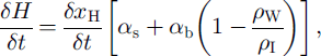
where H is the glacier thickness, α s and α b are, respectively, the surface and basal slopes counted positive pointing upwards, and ρ W and ρ I are, respectively, the sea-water and ice densities. We used ρ W = 1027 kg m−3 and p I = 917 kg m−3 because these values provide a good agreement between ATM ice-shelf elevation above mean sea level and ISR ice thickness. Surface slope, α s, is measured from the KMS DEM (Fig. 9, red color), in the direction of flow. Bedrock slope, α b, is measured from a thickness profile acquired on 19 May 1999 along the center line to be −1.7% (α s is −0.5% at that location, while the thickness gradient, δH/δx, is −2.2%). Assuming by default that α b remains the same from A to B, we used Equation (1) to deduce the ice-thinning rates shown in Figure 9. Ice thinning averages 1.6 ± 1.1 m ice a−1 along the northwestern half of A–B, and 0.6 ± 0.6 m ice a−1 along the southeastern half. The noise level of detection is ± 0.5 m ice a−1.
From the equation of mass continuity (Reference PatersonPaterson, 1994), several interpretations are possible for the observed thinning. One possibility is that snow accumulation decreased or ablation increased. At that elevation, surface accumulation is 0.16 m ice a−1 and ablation 0.9 m ice a−1. These values are unlikely to have changed several hundred per cent in 4 years. Ice thinning therefore cannot be explained by enhanced melting or decreased accumulation. Basal melting, which is 10–20 times larger than surface melting in the 10–20 km seaward of the grounding line, needs to change only by a few per cent (e.g. due to changes in ocean conditions) to trigger thinning of the floating section. Basal melting is, however, negligible at the hinge line, so that another mechanism would be needed to propagate ice thinning upstream of the region of high basal melt.
A more likely interpretation of the retreat is that ice thinning is dynamic, or due to exceptional vertical straining of the ice. Dynamic thinning could result from glacier speed-up caused by enhanced lubrication at the bed or by a reduction in back-stress from a collapsing ice shelf, and entrain a downdraw of the drainage basin. Other East Greenland glaciers seem to exhibit signs of dynamic thinning (Reference KrabillKrabill and others, 1999). Dynamic thinning could be widespread among Greenland’s large outlet glaciers.
Discussion
The mass-budget method suggests that there is more ice draining out of NB and ZI than is accumulated in the interior. Residual uncertainties in surface ablation have a minimal impact on the results since the ice fluxes are calculated well above the region of maximum ablation. Similarly, mass accumulation is poorly constrained by in situ observations, but the addition of new ice cores is not expected to change the mass input estimates significantly, say >5%.
Delineating the glacier drainage basins is a larger source of uncertainty. The boundaries between the three glaciers draining the northeast sector of the Greenland ice sheet are ill-defined from (noisy) surface slope alone. At high elevation, the boundary between ZI and SG runs through the middle of the northeast ice stream. While the ice stream may very well feed more than one glacier system, the result requires confirmation. More reliable or complementary drainage boundaries should be obtainable from a vector mapping of ice velocity over the entire basin using radar interferometry.
Another source of uncertainty in the mass-budget calculations is the role of SG, a surging glacier which is also connected to the northeast ice stream. SG exhibits no ice flux at the grounding line at present (Reference Mohr, Reeh and MadsenMohr and others, 1998) following a surge between 1978 and 1984. SG is thickening upstream of the grounding line. No transverse profile of ice thickness has been collected on SG by NASA’s ISR to measure its ice flux upstream of the zone affected by the surge. If the glacier surges every 70 years and discharges 10.3 km3 ice a−1 for 6 years before returning to a quiescent phase (Reference Reeh, Bøggild and OerterReeh and others, 1994), its average discharge over one surge cycle should be 0.9 km ice a at the grounding line. SG’s balance flux is 4.4 km3 ice a−1 at the grounding line (Table 2). If these estimates are correct, SG exhibits a positive mass balance. The combined grounding-line ice flux of ZI, NB and SG (10.8 + 14.2 + 0.9 = 25.9 km3 ice a−1), however, would exactly balance mass accumulation (25.7 km3 ice a−1 in Table 2), so the three-glacier system as a whole would be in a state of mass balance.
Another estimate of the ice flux of SG may be obtained from the ISR profile collected along the approximate center line of SG on 19 May 1999. Ice thickness is 960 m at 77.4830° N, 23.7589° W (700 m a.s.l). The ice velocity normal to the glacier transverse profile which we selected at that elevation averages 226 m a−1 in our interferometry data, which is consistent with Reference Mohr, Reeh and MadsenMohr and others (1998). Along the shear margins, the ice velocity decreases steeply from 100 m a−1 to zero over a distance of about 5 km on each side. The central region of that profile, where ice velocity is >100 m a−1, is 22 km wide. If we assume ice thickness to be constant in that section, the ice discharge is 4.8 ± 0.4 km3 ice a−1, which is less than half the calculated 10.6 km3 ice a−1 balance discharge at that elevation (not shown in Table 2). Despite the uncertainty of this calculation (no continuous profile of ice thickness), the result tends to confirm that SG exhibits a positive mass balance at that elevation, which could balance mass loss from the two other glaciers. This would suggest that either the drainage-basin boundaries are not correct or some redistribution of mass flow occurred in the past that is not yet well reflected in the ice-sheet topography.
Conclusions
A comparison of balance fluxes with ice discharge suggests that both ZI and NB are in a state of negative mass balance, although the measurement uncertainty remains large, and comparable in magnitude to the calculated imbalance, due to the inherent difficulty of delineating the glacier drainage basins in this sector of Greenland. An independent confirmation of the negative mass budget of NB is provided by the detection of a retreat of its grounding line over a 4 year time period. The corresponding level of ice thinning measured at the grounding line of NB is too large to be caused by temporal changes in ablation and/or accumulation, and must be due to dynamic thinning.
Acknowledgements
This work was performed at the Jet Propulsion Laboratory, California Institute of Technology, under a contract with the NASA Polar Research Program. We thank N. Reeh and an anonymous reviewer for their thoughtful reviews and numerous suggestions which helped improve the paper, C. Werner for use of his SAR processor, and I. Joughin and M. Fahnestock for stimulating discussions about their SAR interferometry project in the interior regions of northeast Greenland.


