


1. Introduction
The stability of a free surface flowing down an inclined plane is a very classical problem that has been widely investigated in the literature. Understanding the mechanism and behaviour of this film instability is of great significance because of its variety of applications in industry, such as enhancing heat and mass transfer rates in process equipment (Brauner & Maron Reference Brauner and Maron1982; Craster & Matar Reference Craster and Matar2009) and coating technology (Weinstein & Ruschak Reference Weinstein and Ruschak2004). The pioneering works of falling films are first discussed experimentally by Kapitza (Reference Kapitza1948, Reference Kapitza1949), who described the development of long-wavelength deformations. Kapitza identified a wide variety of wavy flow regimes, such as the harmonic waves and the solitary waves. Then the linear stability of a gravity-driven film flowing on an inclined plane was derived by Benjamin (Reference Benjamin1957) and Yih (Reference Yih1963) based on the long-wave asymptotic expansion. The results show that the surface instability under the long-wave limitation satisfies  $Re_c=\frac {5}{6}\cot (\beta )$ when the average velocity is used, where $Re_c$ and $\beta$ are the critical Reynolds number and the angle of the inclined plane, respectively. Later, the physical mechanism is investigated by Kelly et al. (Reference Kelly, Goussis, Lin and Hsu1989) using the energy method. They show that the dominant energy production term is associated with the work done by the perturbation shear stress at the free surface, and the mechanism of instability is linked to a perturbation vorticity shift relative to the surface displacement caused by advection. On the other hand, another mode called the shear mode has been discovered. It appears only when the Reynolds number is high and the inclined angle is very small, which differs from the surface mode (Lin Reference Lin1967; Bruin Reference Bruin1974; Chin, Abernath & Bertschy Reference Chin, Abernath and Bertschy1986; Floryan, Davis & Kelly Reference Floryan, Davis and Kelly1987).
Inevitably, wall oscillation sometimes occurs in the practical production process. It is even necessary to introduce appropriate wall oscillation in some processes. For the oscillating plane, the asymptotic expansion was first introduced by Yih (Reference Yih1968) to discuss the long-wave surface instability of Newtonian flow on a horizontal plane. The Floquet theory is utilized to resolve the time-dependent Orr–Sommerfeld boundary problem. Results show that the oscillatory instability mode is found to be unstable or stable depending on the oscillation frequency. Or (Reference Or1997) extended the long-wave instability results to finite-wavelength instability. He found that the long-wave unstable neutral curve exhibits a U-shaped distribution in discrete oscillatory frequencies over an arbitrary range of wavenumbers, while the finite-wavelength neutral curve separates from the bifurcation point of the U-shaped curve to exhibit a diagonal intersection line, and occupies the stability window of the long wave. For an inclined oscillating plate, Woods & Lin (Reference Woods and Lin1995) numerically investigated the instability with arbitrary wavenumbers. Three types of instabilities are identified for the Newtonian fluid flowing down an inclined plane, which are the gravity unstable region corresponding to the surface mode, and two types of resonance waves/Faraday waves: the subharmonic wave and harmonic wave. They concluded that the wall-normal oscillation can suppress the gravity instability but intensify the resonance waves, and both surface waves and shear waves are quickly dominated by the resonance waves, with the oscillating amplitude increasing. Later, Lin, Chen & Woods (Reference Lin, Chen and Woods1996) discussed the instability characteristics for a streamwise oscillating plane. Two types of instabilities associated with harmonic instability and gravity instability appear. The streamwise oscillation shows a suppression effect to the gravity instability, and the onset of instability becomes harmonic instability from gravity instability. Recently, this work has been followed by Jaouahiry & Aniss (Reference Jaouahiry and Aniss2020), which focuses on the effect of the insoluble surfactants. It is found that the insoluble surfactants suppress gravity instability and resonance instability. By introducing the shear stress on the surface liquid film, Samanta (Reference Samanta2021) found that the gravitational and shear instabilities can be amplified with the increasing value of imposed shear stress for both the cross-stream oscillatory flow and the stream oscillatory flow cases.
In all of the aforementioned studies, the authors focused primarily on the stability of Newtonian liquid flow. Research on non-Newtonian liquid flow has also been intensified due to its wide usage in chemical industry. Generally, non-Newtonian fluids can be divided into three categories: (a) time-independent (memoryless), (b) time-dependent and (c) viscoelastic. For time-independent fluids, the strain rate at a given position is based solely on the current value of the shear stress at that point. Power-law fluid and viscoplastic fluid are typical examples of memoryless fluid. For time-dependent fluids, the relation between the shear stress and strain rate shows dependence on the duration of kinematic and shearing history, e.g. thixotropic fluid. Viscoelastic fluids are a type of non-Newtonian fluid exhibiting features that are typical of both viscosity and elasticity. There are many different constitutive models of viscoelasticity, such as the second-order liquid, the Walters’ liquid  $B''$, the Maxwell liquid and the Oldroyd-B liquid, describing the distinct rheological behaviours. In second-order fluid models, the typical fluid relaxation time is very small compared with the characteristic time scale of the flow, i.e. the Deborah number should be much less than one. The Maxwell model is a linear differential model of viscoelastic fluids, which is applicable for the case of the deformation gradients being infinitesimally small. At moderate shear rates, Oldroyd-B is the widely used model to study the effects of viscoelasticity in shear flows of highly elastic dilute liquids. In this paper, Walters’ liquid $B''$ is considered as the rheological model, which is the approximation of neglecting second-order terms in relaxation time and retardation time of the Oldroyd-B model. Thus Walters’ liquid $B''$ can describe only weak viscoelasticity and has a short or rapidly fading memory. Here, the rapidly fading memory can be thought as a physical property of a weakly viscoelastic liquid that causes it to forget its distant past history of deformations (Samanta Reference Samanta2023).
It is observed that the effect of viscoelastic liquid has a noticeable impact on promoting instability. For example, the viscoelastic parameter has a destabilizing effect on the surface mode for the case of inclined plane without oscillating (Gupta Reference Gupta1967; Wei Reference Wei2005; Pal & Samanta Reference Pal and Samanta2021). For the viscoelastic liquid film on a horizontal oscillating plane, Dandapat & Gupta (Reference Dandapat and Gupta1975) first investigated the long-wave instabilities induced by the streamwise oscillation. The results show that the stability is destabilized and stabilized in different ranges of frequency. Samanta (Reference Samanta2017) extended the long-wave regime to the arbitrary-wavelength regime. It is shown that the finite-wavelength instability is more dangerous than the long-wave instability under specific frequencies. More recently, the effect of insoluble surfactants on the linear instability of viscoelastic film on an oscillating plane for disturbances with arbitrary wavenumbers has been investigated by Wang et al. (Reference Wang, Du, Xiao and Zhao2023). However, there is little research on the analysis of long-wave limit stability and finite-wavelength instability for viscoelastic film flows on an oscillating inclined plane. More importantly, it is unknown how the oscillation amplitude in the streamwise and wall-normal directions and viscoelasticity affect the onset of instabilities in this system, which is the main motivation of this paper. The remainder of this investigation is outlined as follows. In § 2, the governing equations of the fluid problem are described. The results of long-wavelength instability are presented in § 3. The results of finite-wavelength instability are discussed in § 4. Finally, conclusions are presented in § 5.
2. Mathematical formulation
2.1. Flow configuration
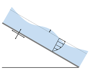
We consider a two-dimensional incompressible viscoelastic liquid film flowing down an inclined plane making an angle  $\theta$ with the horizontal, as shown in figure 1. The thickness of liquid film is $2d$, and the origin of the Cartesian coordinate system is placed in the middle of the unperturbed liquid film. The inclined plate is forced to oscillate sinusoidally in the streamwise direction ( $x$-axis) and wall-normal direction ( $\kern 1.5pt y$-axis), with constant frequency $\omega$. The solid line $h(x,t)$ shows the deformed liquid surface. For a given viscoelastic liquid, the density $\rho$ is assumed to be constant. Also, the amplitudes of oscillation in the streamwise and wall-normal directions are $A_x$ and $A_y$. According to the d’Alembert theorem, the governing equations in a non-inertial reference system can be expressed as
 $$\begin{gather} \partial_x u+\partial_y \upsilon =0, \end{gather}$$
 $$\begin{gather}\rho(\partial_t u + u\,\partial_x u+\upsilon\,\partial_y u)= \partial_x\tau_{xx}+\partial_y\tau_{xy}+\rho g\sin\theta - \rho A_x \omega^2\sin\omega t, \end{gather}$$
 $$\begin{gather}\rho(\partial_t \upsilon + u\,\partial_x \upsilon + \upsilon\,\partial_y \upsilon)=\partial_x\tau_{y x}+\partial_y\tau_{y y} -\rho g\cos\theta - \rho{A_y \omega^2}\sin\omega t, \end{gather}$$
where  $u$ and $\upsilon$ are velocity components in the streamwise and wall-normal directions, respectively. The inertial forces in two directions are expressed as $\rho A_x \omega ^2\sin \omega t$ and $\rho A_y \omega ^2\sin \omega t$. Here, $g$ is the gravitational acceleration, and $\tau _{ij}$ is the component of the stress tensor, with different expressions for different viscoelastic fluids. Walters’ liquid $B''$ is used in this paper, which represents an approximation to first order in elasticity, i.e. for short or rapidly fading memory fluids, and satisfies the following constitutive equation of state (Beard & Walters Reference Beard and Walters1964; Andersson & Dahl Reference Andersson and Dahl1999):
 \begin{equation} \tau_{i j} ={-}p\delta_{i j} + 2\mu e_{ij}-2M_0\,\frac{\delta}{\delta t}\,e_{ij}, \end{equation}
where  $\mu$ is the limiting viscosity, $e_{ij}=(\partial _{i}u_j + \partial _j u_i)/2$ is the strain rate tensor, $2\mu e_{ij}$ corresponds to the Newtonian stress, $2M_0(\delta /\delta {t})e_{i j}$ corresponds to elastic stress, $M_0$ is the viscoelastic coefficient, $\delta _{i j}$ is the Kronecker symbol, and $p$ is the isotropic pressure. Walters’ liquid $B''$ is chosen because the constitutive equation of this model involves only one non-Newtonian parameter, although this model can describe only shear flows of weakly elastic dilute liquids. The advantages brought by this are that one can easily obtain a deeper insight into the flow behaviour of viscoelastic fluids. Besides, Walters’ liquid $B''$ with limiting viscosity at low shear rates and short memory coefficient is one of the best models to describe the characteristics of a viscoelastic fluid. Nevertheless, it should be noted that Walters’ liquid $B''$ is an approximation to the Oldroyd-B liquid in the limit of small relaxation time. And the flow needs to have the characteristics of low shear rates and weak viscoelasticity when using the constitutive equation. This approximation is reasonable for analysing the flow similar to the boundary layer and liquid film. For typical parameters of Walters’ liquid $B''$ (Walters Reference Walters1960), a mixture of polymethyl methacrylate in pyridine has density $\rho = 0.98\times 10^3\,\mathrm {kg}\,\mathrm {m}^{-3}$, limiting viscosity $\mu = 0.79\,\mathrm {N}\,\mathrm {s}\,\mathrm {m}^{-2}$, and viscoelastic coefficient $M_0 = 0.04\,\mathrm {N}\,\mathrm {s}^{2}\,\mathrm {m}^{-2}$. The upper convected derivative for the strain rate tensor is defined as
 \begin{equation} \frac{\delta}{\delta t}\,e_{ij}=\partial_t e_{ij}+u_k\,\partial_k e_{ij}- \partial_k u_j e_{ik}-\partial_k u_i e_{kj}. \end{equation}
Figure 1. Schematic of a viscoelastic fluid on an oscillating inclined plane.
For the boundary conditions, it satisfies no-slip and no-penetration at  $y = -d$ since the coordinate system is fixed at the oscillating plate:
 \begin{equation} u=0,\quad \upsilon=0. \end{equation}
The free surface of the film at  $y=d+h(x,t)$ satisfies the normal force conservation, zero tangential force conservation and kinematic boundary condition:
 $$\begin{gather} p_a + \tau_{i j} n_i n_j =\sigma\,\frac{ \partial_{xx} h } {(1+\partial_x^{2}h)^{3/2}}, \end{gather}$$
 $$\begin{gather}\tau_{i j} n_j t_i =0, \end{gather}$$
 $$\begin{gather}\partial_{t} h + u\,\partial_{x} h = \upsilon, \end{gather}$$
where  $\sigma$ is the surface tension, $\boldsymbol {n}$ is the unit normal vector, $\boldsymbol {t}$ is the unit tangent vector, and $p_{a}$ is the ambient pressure. It is assumed that there is no external force on the surface of the liquid film, e.g. imposed shear stress, so the tangent stress of the free surface is equal to zero. Then the governing equations and boundary conditions are normalized by introducing $d$ as the length scale, $1/\omega$ as the time scale, $d\omega$ as the velocity scale, and $\rho \omega ^2 d^2$ as the pressure scale. The choice of characteristic time scale can be varied. Considering that the research object of this work is the influence of an oscillating boundary on the flow of a liquid film on an inclined plate, from this point of view, $1/\omega$ is more suitable. If only the influence of the inclined angle on the flow field is discussed, then it is more appropriate to use the liquid film thickness divided by the typical velocity as the time scale. The dimensionless parameters of the problem are as follows: the Reynolds number ${{Re}} =\omega d^2/\nu$ shows the effect of frequency; the Froude number $Fr=\omega d/\sqrt {gd}$ shows the effect of gravity; the Weber number $We=\sigma /\rho \omega ^2 d^3$ shows the effect of surface tension, and the viscoelastic parameter $M=M_0/(\rho d^2)$ shows the effect of viscoelasticity.
For the basic flow, we consider a unidirectional parallel flow, and the unperturbed surface of the viscoelastic liquid film is parallel to the plate at  $y = 1$. By simplifying the governing equations and boundary conditions in a reference frame moving with the oscillating inclined plate, the dimensionless equations for the basic flow are obtained:
 $$\begin{gather} \partial_{t}U ={-}\partial_{x}P + {{Re}}^{{-}1}\,\partial_{yy}U - M\,\partial_{yyt}U + \frac{\sin\theta}{Fr^{2}} -a_{x} \sin t, \end{gather}$$
 $$\begin{gather}0=\partial_{y}P+\frac{\cos\theta}{Fr^{2}}+a_{y}\sin t, \end{gather}$$
with the corresponding boundary conditions
 $$\begin{gather} U=0,\quad\text{at}\ y={-}1, \end{gather}$$
 $$\begin{gather}\partial_{y}U - M\,Re\,\partial_{yt}U=0,\quad P=P_{a},\quad \text{at}\ y=1, \end{gather}$$
where  $U(y,t)$ is the velocity of basic flow, $P=p_a/\rho (\omega d)^2$ is the dimensionless ambient pressure, and $a_x=A_x/d$ and $a_y=A_y/d$ are the oscillation amplitude components in the streamwise and wall-normal directions, respectively. By solving unperturbed parallel flow (2.10)–(2.11), the theoretical solution can be expressed as
 \begin{gather} U(y,t) = U^s(y) +
U^t(y,t) \nonumber\\
=
\frac{{{Re}}\sin\theta}{2\,Fr^2}\,(3+2y-y^2)
- a_x\,\mathrm{Re} \left[\left\{\frac{\cosh[r
(y-1)]}{\cosh(2r)}-1 \right\}\text{e}^{\text{i}t}\right],
\end{gather}
\begin{gather} U(y,t) = U^s(y) +
U^t(y,t) \nonumber\\
=
\frac{{{Re}}\sin\theta}{2\,Fr^2}\,(3+2y-y^2)
- a_x\,\mathrm{Re} \left[\left\{\frac{\cosh[r
(y-1)]}{\cosh(2r)}-1 \right\}\text{e}^{\text{i}t}\right],
\end{gather} $$\begin{gather} P(y,t)=P_{a}+\left(\frac{\cos\theta}{F r^{2}}+a_{y}\sin t\right)(1-y), \end{gather}$$
 $$\begin{gather}V(y,t)=0, \end{gather}$$
with
 \begin{equation} \left.\begin{gathered} r=\sqrt{\frac{\text{i}\,{{Re}}}{1 - \text{i}M\,{{Re}}}} ={\pm} \varOmega\sqrt{{{Re}}\,S/2}\,(1+\mathrm{i}S),\\ \varOmega=\frac{\sqrt{1+(M\,{{Re}})^2}-M\,{{Re}}}{\sqrt{1+(M\,{{Re}})^2}},\\ S=\sqrt{1+(M\,{{Re}})^2} + M\,{{Re}}, \end{gathered}\right\} \end{equation}
where  $\mathrm {Re}[\cdot ]$ represents the real part of a complex function. The basic flow is separated into two parts, namely, the steady part denoted by $U^s(y)$ and the time-dependent flow denoted by $U^t(y,t)$. Note that wall-normal oscillation $a_y$ is involved only in the expression for pressure, which means that the unperturbed velocity is independent of wall-normal oscillation. Besides, the discussed problem degenerates into that of Woods & Lin (Reference Woods and Lin1995) and Lin et al. (Reference Lin, Chen and Woods1996) if the viscoelastic parameter $M$ is zero. Further setting the oscillation amplitudes to zero, the basic flow will degenerate into the stability problem of the Newtonian fluid discussed by Yih (Reference Yih1963).
2.2. Linear stability problem
Considering the linear stability problem, the linear time-dependent Orr–Sommerfeld equations can be derived by introducing the infinitesimal perturbation to the basic flow. By ignoring higher-order small quantities, the perturbed flow variables can be expressed as
 \begin{equation} u=U+u',\quad \upsilon=\upsilon',\quad p=P+p',\quad h=1+h', \end{equation}
where variables with superscript prime denote perturbation variables. By substituting perturbation variables (2.16a–d) into the governing equations and boundary conditions (2.10)–(2.11), we can obtain the dimensionless perturbation equations. Considering only the onset of instability with respect to two-dimensional disturbance, the continuity will be automatically satisfied by introducing a streamfunction  $\psi '(x,y,t)$, such that
 \begin{equation} u'=\partial_{y}\psi',\quad \upsilon'={-}\partial_{x}\psi'. \end{equation}
In the following stability analysis, we look for the normal mode solution of the form
 $$\begin{gather} \psi'(x,y,t)={\phi}(y,t)\,\mathrm{e}^{\mathrm{i}k x}, \end{gather}$$
 $$\begin{gather}h'(x,t)=\eta(t) \,\mathrm{e}^{\mathrm{i}k x}, \end{gather}$$
where  $k$ represents the wavelength of infinitesimal perturbation in the streamwise direction. By substituting the normal mode solution into the dimensionless perturbation equations, one can derive the time-dependent Orr–Sommerfeld equation as
 \begin{equation} (\mathscr{L}+M \mathscr{L}^{2})\,\partial_{t} \phi = \mathscr{L}^{2} \phi/{{Re}}-\mathrm{i} k U(\mathscr{L}+M \mathscr{L}^{2})\phi + \mathrm{i} k(\mathscr{D}^{2} U+M \mathscr{D}^{4} U) \phi, \end{equation}
with boundary conditions
 \begin{align} \phi&=\mathscr{D} \phi=0,\quad \text{at}\ y={-}1, \end{align}
 \begin{align} M\,{{Re}}\,(\mathscr{L}+2 k^{2})\,\partial_{t} \phi &= (\mathscr{L}+2 k^{2}) \phi -\mathrm{i}kM\,{{Re}}\,[U(\mathscr{L}+2 k^{2})-\mathscr{D}^{2} U] \phi \nonumber\\ &\quad +[\mathscr{D}^{2} U- M\,{{Re}}\,\mathscr{D}^{2}\,\partial_{t} U]\eta,\quad \text{at}\ y=1, \end{align}
 \begin{align} \hbox{[}\mathscr{D}+M(\mathscr{L}-2 k^{2})\mathscr{D}]\,\partial_{t} \phi &= (\mathscr{L}-2 k^{2}) \mathscr{D} \phi/{{Re}}-\mathrm{i} k\eta(\cos{\theta}/Fr^2+a_y\sin{t} +k^{2}\,We) \nonumber\\ &\quad -\mathrm{i} k\{U[\mathscr{D}+M(\mathscr{L}-2 k^{2}) \mathscr{D}] \nonumber\\ &\quad +M(\mathscr{D}^{2} U \mathscr{D}-\mathscr{D}^{3} U)\} \phi,\quad \text{at}\ y=1, \end{align}
 \begin{align} \partial_{t} \eta&={-}\mathrm{i} k \phi-\mathrm{i} k U \eta,\quad \text{at}\ y=1, \end{align}
where the linear operators are  $\mathscr {L}=\mathscr {D}^2- k^2$ and $\mathscr {D}=\partial _y$. The Floquet system (2.20)–(2.21) governs the linear stability problem. For finite-wavelength instabilities, the differential system should be solved numerically, while long-wavelength solutions can be obtained analytically by an expansion in $k$, and will be discussed in the following.
3. The long-wavelength expansion
For wavelengths that are long compared with the thickness of film  $2d$, the disturbed wavenumber $k$ is small, and the Floquet system with periodic coefficients is resolved based on the long-wavelength expansion ( $k \ll 1$) along with the Floquet theory proposed by Yih (Reference Yih1968). Under the limit of long waves, the solution is assumed in the form
 $$\begin{gather} \phi(y,t) = \mathrm{e}^{\gamma t}\,[\phi_0(y,t) + k\,\phi_1(y,t) + k^2\,\phi_2(y,t) + \cdots], \end{gather}$$
 $$\begin{gather}\eta(t) = \mathrm{e}^{\gamma t}\,[\eta_0(t) + k\,\eta_1(t) + k^2\,\eta_2(t) + \cdots], \end{gather}$$
where the eigenfunctions  $\phi _j(y,t)$ and $\eta _j(t)$ ( $\kern 1.5pt j = 0, 1, 2,\ldots$) are $2{\rm \pi}$-periodic in time, the Floquet exponent $\gamma = \gamma _r + \mathrm {i}\gamma _i$ is the complex growth rate of the disturbance, and $\gamma$ is expanded as a power series in $k$:
$k$:
 \begin{equation} \gamma = \gamma_0+k\gamma_1+k^2\gamma_2+\cdots. \end{equation}
The imaginary part of the Floquet exponent represents the phase difference, while the real part represents the growth rate. By substituting expansion (3.1) into the Floquet system (2.20)–(2.21), and collecting different order terms, a set of coupled ordinary differential equations can be derived. By solving each order differential system, a series of Floquet exponents  $\gamma _j$ ( $\kern 1.5pt j=1,2,\ldots$) can be obtained until the first non-zero growth rate is found.
For the first-order  $O(k^0)$, the Floquet system can be simplified as
 \begin{equation} (\mathscr{D}^2+M\mathscr{D}^4)\,\partial_t\phi_0 = \mathscr{D}^4\phi_0/{{Re}}, \end{equation}
with boundary conditions
 $$\begin{gather} \phi_0 = \mathscr{D}\phi_0=0, \quad \text{at}\ y={-}1 , \end{gather}$$
 $$\begin{gather}M\,{{Re}}\,\mathscr{D}^2\,\partial_t \phi_0-\mathscr{D}^2 \phi_0 = (\mathscr{D}^2 U - M\,{{Re}}\,\mathscr{D}^2\,\partial_t U)\eta_0,\quad \text{at}\ y=1, \end{gather}$$
 $$\begin{gather}(\mathscr{D} + M \mathscr{D}^3 )\,\partial_t \phi_0=\mathscr{D}^3 \phi_0/{{Re}},\quad \text{at}\ y=1, \end{gather}$$
 $$\begin{gather}\gamma_0\eta_0 + \partial_t\eta_0=0, \quad \text{at}\ y=1. \end{gather}$$
 Here,  $\gamma _0$ must be zero since $\eta _0(t)$ is a periodic function of $t$. Otherwise, $\eta =0$ and $\gamma _0\ne 0$ will lead to a damped mode as far as long waves are concerned, and that damped mode is not of interest here. Without loss of generality, we choose $\eta _0=1$. It can be noted that the basic flow $U(y,t)$ consists of a steady part $U^s(y)$ and a time-dependent part $U^t(y,t)$, mainly reflected in the tangential boundary condition in (3.4). Therefore, the solution can be assumed to be
 \begin{equation} \phi_0(y,t) = \bar{\phi}_0(y) + \tilde{\phi}_0(y,t), \end{equation}
where  $\bar {\phi }_0(y)$ and $\tilde {\phi }_0(y,t)$ represent the solutions induced by the steady and time-dependent parts of the basic flow, respectively. By inserting $\phi _0(y,t)$ into (3.3)–(3.4) and solving for the first-order Floquet systems of $\bar {\phi }_0(y)$ and $\tilde {\phi }_0(y,t)$, one can get the solution expression as
 $$\begin{gather} \bar{\phi}_0 = \frac{{{Re}}\sin{\theta}}{2\,Fr^2}\,(1 + y)^2, \end{gather}$$
 $$\begin{gather}\tilde{\phi}_0 = a_x\, \mathrm{{{Re}}}\left[\frac{\cosh(r(y+1))-1}{\cosh^2(2r)}\,\text{e}^{\text{i}t}\right]. \end{gather}$$
 Obviously, the inclined angle  $\theta$ affects only $\bar {\phi }_0$, which is induced by gravity and does not affect $\tilde {\phi }_0$, which is induced by streamwise oscillation $a_x$. The surface kinematic equation of the first-order Floquet system can also be obtained by collecting $O(k)$ terms:
 \begin{equation} \gamma_1 + \partial_t\eta_1 ={-}\mathrm{i}( \phi_0 + U ). \end{equation}
Taking the steady terms and time-dependent terms for both sides of (3.7), one can obtain expressions for  $\gamma _1$ and $\eta _1(t)$ as
 $$\begin{gather} \gamma_1 ={-}4\mathrm{i}\,{{Re}}\sin{\theta}/Fr^2, \end{gather}$$
 $$\begin{gather}\eta_1 ={-}\mathrm{i}a_x\, \mathrm{Im}\left[\left(1-\frac{1}{\cosh^2{(2r)}}\right)\mathrm{e}^{\mathrm{i}t}\right], \end{gather}$$
where  $\mathrm {Im}[\cdot ]$ represents the imaginary part of a complex function. Here, $\gamma _1$ is a pure imaginary number and is induced only by $x$-direction components of gravity. If the characteristic velocity scale $\omega d$ is replaced by a new velocity $u_a =4gd^2\sin {\theta }/3\nu$, then the dimensionless parameters $Fr$ and ${{Re}}$ will have the relation $3\,Fr^2=4\,{{Re}}\sin {\theta }$. Then the expression for $\gamma _1$ can be rewritten as $-3\mathrm {i}$, which is in agreement with the typical result for an inclined plane without oscillation (Yih Reference Yih1963).
To further determine the stability of the system, the order  $O(k^2)$ for the Floquet system should be discussed. As the Floquet exponent $\gamma _2$ is independent of time, the solution of first-order steady equations is sufficient to compute the next order Floquet exponent. Therefore, we will focus solely on the steady terms of the first-order system. For the first-order steady system of $\bar {\phi }^s_1(y)$ induced by gravity, we have the set of equations
 \begin{equation} (\mathscr{D}^{2}+M \mathscr{D}^{4})\gamma_{1} \bar{\phi}_0 = \mathscr{D}^{4} \bar{\phi}^s_1/{{Re}}-\mathrm{i}U^s(\mathscr{D}^{2}+M \mathscr{D}^{4}) \bar{\phi}_0 +\mathrm{i}(\mathscr{D}^{2} U^s+M \mathscr{D}^{4} U^s) \bar{\phi}_0, \end{equation}
with boundary conditions
 $$\begin{gather} \bar{\phi}^s_1 = \mathscr{D} \bar{\phi}^s_1 = 0,\quad \text{at}\ y ={-}1, \end{gather}$$
 $$\begin{gather}M\,{{Re}}\,\mathscr{D}^{2}\gamma_1 \bar{\phi}^s_0 = \mathscr{D}^{2} \bar{\phi}^s_{1}- \mathrm{i}M\,{{Re}}\,(U^s \mathscr{D}^{2}-\mathscr{D}^{2} U^s) \bar{\phi}^s_{0},\quad \text{at}\ y = 1, \end{gather}$$
 \begin{gather} (\mathscr{D}+M \mathscr{D}^{3})\gamma_1 \bar{\phi}^s_0 = \mathscr{D}^{3} \bar{\phi}^s_{1}/{{Re}} -\mathrm{i}(\cos{\theta}/Fr^2+k^2\,We) -\mathrm{i}U^s(\mathscr{D}+M \mathscr{D}^{3})\bar{\phi}^s_{0} \nonumber\\ \qquad \qquad -\mathrm{i}M(\mathscr{D}^{2} U^s \mathscr{D}-\mathscr{D}^{3} U^s) \bar{\phi}^s_{0},\quad \text{at}\ y = 1. \end{gather}
 For the first-order system of  $\tilde {\phi }^s_1(y)$ induced by oscillation, we have the set of equations
 \begin{equation} \mathscr{D}^{4} \tilde{\phi}^s_1/{{Re}}= \mathrm{i}[U^t(\mathscr{D}^{2}+M \mathscr{D}^{4}) \tilde{\phi}_0-(\mathscr{D}^{2} U^t+M \mathscr{D}^{4} U^t)\tilde{\phi}_0]^s, \end{equation}
with boundary conditions
 $$\begin{gather} \tilde{\phi}^s_1 = \mathscr{D} \tilde{\phi}^s_1 = 0,\quad \text{at}\ y ={-}1, \end{gather}$$
 $$\begin{gather}\mathscr{D}^{2} \tilde{\phi}^s_{1} = \mathrm{i}M\,{{Re}}\,(U^t \mathscr{D}^{2}-\mathscr{D}^{2} U^t) \tilde{\phi}^s_{0} + (\mathscr{D}^{2} U^t- M\,{{Re}}\,\mathscr{D}^{2}\,\partial_{t} U^t)\eta_1,\quad\text{at}\ y = 1, \end{gather}$$
 $$\begin{gather}\mathscr{D}^{3} \tilde{\phi}^s_{1}= \mathrm{i}\,{{Re}}\,[U^t(\mathscr{D}+M \mathscr{D}^{3})+M(\mathscr{D}^{2} U^t \mathscr{D}-\mathscr{D}^{3} U^t)] \tilde{\phi}^s_{0},\quad \text{at}\ y = 1. \end{gather}$$
 After some mathematical manipulation, the solution of the first-order steady system of  $\bar {\phi }^s_1(y)$ can be expressed as
 \begin{equation} \bar{\phi}^s_{1} = \mathrm{i}\,\frac{{{Re}}^3\sin^2{\theta}}{Fr^4} \left(\frac{y^5}{60} - \frac{y^4}{12}\right) + \bar{A}y^3 + \bar{B}y^2 +\bar{C}y +\bar{D}, \end{equation}
with
 \begin{equation} \left.\begin{gathered} \bar{A} = \mathrm{i}\,\frac{{{Re}}^3\sin^2{\theta}}{Fr^4}\left(-\frac{1}{2} - \frac{1}{3}\,M\right) + \frac{\mathrm{i}}{6}\,{{Re}}\left(\frac{\cos{\theta}}{Fr^2}+ k^2\,We\right), \\ \bar{B} = \mathrm{i}\, \frac{{{Re}}^3\sin^2{\theta}}{Fr^4}\left(\frac{11}{6} + M\right) - \frac{\mathrm{i}}{2}\,{{Re}}\left(\frac{\cos{\theta}}{Fr^2}+ k^2\,We\right), \\ \bar{C} = \mathrm{i}\,\frac{{{Re}}^3\sin^2{\theta}}{Fr^4}\left(\frac{19}{4} + 3M\right) - \frac{\mathrm{3i}}{2}\,{{Re}}\left(\frac{\cos{\theta}}{Fr^2}+ k^2\,We\right), \\ \bar{D} = \mathrm{i}\,\frac{{{Re}}^3\sin^2{\theta}}{Fr^4}\left(\frac{151}{60} + \frac{5}{3}\,M\right) - \frac{\mathrm{5i}}{6}\,{{Re}}\left(\frac{\cos{\theta}}{Fr^2}+ k^2\,We\right). \end{gathered}\right\} \end{equation}
The solution of the first-order unsteady system of  $\tilde {\phi }^s_1(y)$ can be expressed as
 \begin{equation} \tilde{\phi}^s_1 = \mathrm{i}\,\frac{a_x^2}{2}\,R_1 + \mathrm{i}\,\frac{a_x^2}{2}\,R_2 + \tilde{A}y^3 + \tilde{B}y^2 + \tilde{C}y + \tilde{D}, \end{equation}
with
 \begin{equation} \left.\begin{aligned} R_1&= \frac{-(a^4 -6a^2 b^2 +b^4)}{8a^4 b^4 {{[\cosh (4a)+\cos (4b)]}}^2} \\ &\quad\times \{a^4 \sin [2b{(y-1)}] \sinh (4a)+b^4 \sinh [2a{(y-1)}]\sin (4b)\}, \\ R_2&= \mathrm{Re}\left[\mathrm{i}\,\frac{\cosh [{(a-b\mathrm{i})}{(y+1)}]}{{\cosh^2 (2a-2b\mathrm{i})}} + \mathrm{i}\,\frac{\cosh [{(a+b\mathrm{i})}{(y-1)}]}{{\cosh^2 (2a-2b\mathrm{i})}\cosh (2a+2b\mathrm{i})}\right], \\ \tilde{A} &= \tilde{B} = 0, \\ \tilde{C} &={-}\mathrm{i}\,\frac{a_x^2}{2}\,(\mathscr{D}R_1 + \mathscr{D}R_2)|_{y={-}1}, \\ \tilde{D} &={-}\mathrm{i}\,\frac{a_x^2}{2}\,(\mathscr{D}R_1 + R_1 +\mathscr{D}R_2 + R_2)|_{y={-}1}, \end{aligned}\right\} \end{equation}
where  $a, b$ are the real and imaginary parts of $r$, respectively:
 \begin{equation} a=\varOmega\sqrt{Re\,S/2},\quad b=\varOmega S \sqrt{Re\,S/2}. \end{equation}
 Substituting (3.1) into (2.21d) and collecting  $O(k^2)$ terms, the surface kinematic equation of the second-order Floquet system can be obtained as
 \begin{align} \gamma_2 &={-}\mathrm{i} [\bar{\phi}^s_1 + \tilde{\phi}^s_1 + U^t\eta_1] \nonumber\\ &={-} \mathrm{i} \bar{\phi}^s_1|_{y=1} - a_x^2\left.\left[\mathscr{D}R_1 + \frac{R_1}{2} + \mathscr{D}R_2 + \frac{R_2}{2}\right]\right|_{y={-}1}, \end{align}
with
 \begin{equation} - \mathrm{i}\bar{\phi}^s_1|_{y=1}= \frac{{{Re}}^3\sin^2{\theta}}{Fr^4} \left(\frac{128}{15} + \frac{16}{3}\,M\right) - \frac{8}{3}\,{{Re}} \left(\frac{\cos{\theta}}{Fr^2}+ k^2\,We\right). \end{equation}
 From (3.19), we conclude that the stability of a long-wave system consists of the gravity-related item  $\bar {\phi }^s_1|_{y=1}$ and the streamwise oscillation related terms $R_1$ and $R_2$. In other words, the long-wave solution is independent of the wall-normal oscillation amplitude $a_y$. If streamwise oscillation $a_x$ equals zero, then the stability of the system is dependent only on $- \mathrm {i} \bar {\phi }^s_1|_{y=1}$.
Up to now, we have obtained the analytical solution of the linear stability of the viscoelastic fluid film on the inclined plate under the long-wave limit. Based on the theoretical solution, we will analyse the dependence of liquid film stability with different parameters, including the inclination angle  $\theta$, viscoelastic parameters $M$, Froude number $Fr$, Reynolds number ${{Re}}$, and Weber number $We$. Before this, as a supplement and support to the theoretical results, the finite-wavelength analysis is also performed by solving the time-dependent disturbance equation. The relevant numerical procedure is introduced in detail in Wang et al. (Reference Wang, Du, Xiao and Zhao2023), and will not be repeated here. Several tests are performed for different numbers of Chebyshev polynomials and Fourier series to ensure numerical convergence, and the results are shown in Appendix A.
Under the limit of long waves ( $k \ll 1$), the analytical solution and numerical solution are compared with different oscillatory amplitudes and viscoelastic values. Figure 2(a) displays the real part $\gamma _r$ and the imaginary part $\gamma _i$ for Newtonian fluid in the range $10^{-8}< k<10^{0}$ by taking the typical parameters $We=0.016$, $\theta =90^\circ$, $Fr=10$, $a_y=0.1$, ${{Re}}=5$. It can be seen that the Floquet exponent is complex-valued. The real part of the eigenvalue $\gamma$ is always positive, which eventually leads to the unstable system of the flow. It can be noted that the numerical solution (blue open circles) and the analytical solution (black solid lines) match very well when the wavenumber $k$ is smaller than $10^{-1}$. For a larger wavenumber, the assumption of a long-wave limit is no longer valid, and the analytical solutions will gradually become invalid. Figure 2(b) displays the real part $\gamma _r$ of viscoelastic fluid varying with the wavenumber $k$ under the same range $10^{-8}< k<10^{0}$ with the given parameters $We=0.016$, $\theta =90^\circ$, $Fr=100$, $a_x=6$, ${{Re}}=10$. The lower and upper lines are the long-wave solutions with viscoelastic parameters $M=0$ and $M=0.01$, respectively. It can be seen that the viscoelasticity has a destabilizing effect on the instability under the given parameters. Similarly, the blue open circles coincide well with the black solid line in the range $k<10^{-2}$. When $k>10^{-1}$, the long-wave solution gradually deviates from the numerical solution, which indicates the correctness of the long-wave solution and numerical solution for streamwise oscillation. It will be seen below that this instability falls within the oscillatory instability range. In this section, the numerical results will be used only to verify the rationality of the long-wave theoretical analysis, and ensure the correctness and determine the applicability of the theoretical solution. All results discussed below in this part are based on the theoretical solutions.

Figure 2. (a) Comparison of long-wave analytical solutions (black lines) and numerical solutions (blue open circles) for a Newtonian fluid with flow parameters  $Fr=10$, $M=0$, $a_x=0$, $a_y=0.1$, ${{Re}}=5$, $We=0.016$ and $\theta =90^\circ$. (b) Comparison of long-wave analytical solutions (black lines) and numerical solutions (blue open circles) for viscoelastic fluid with flow parameters $Fr=100$, $a_x=6$, $a_y=0$, ${{Re}}=10$, $We=0.016$ and $\theta =90^\circ$.
3.1. Effect of inclined angle ( $M = 0$, $We=0.016$, $Fr = 100$)


First, we calculated the distribution of unstable regions on the  $(a_x, {{Re}})$-plane at different dip angles when there is no viscoelasticity ( $M=0$), as shown in figure 3. The stable and unstable regions are denoted by blue and yellow, respectively. When the inclination angle is small ( $\theta <50^{\circ }$), as can be seen from figures 3(a,b), the unstable region presents three families of U-shaped curves (from low-frequency to high-frequency, the first, second and third families in turn), and the flow will be unstable only within a specific ${{Re}}$ range. With the increase of oscillation frequency, the amplitude of oscillation leading to linear instability is also increasing rapidly. Nevertheless, when the inclination angle is in the range $10^{\circ }$– $50^{\circ }$, the instability boundary has hardly changed. When $\theta =60^{\circ }$, a new unstable region appears at the high-frequency oscillation ( ${{Re}}>45.6$) in figure 3(c), and a very small amplitude of streamwise oscillation in this region can also make the flow unstable. After careful examination, the instability of this area is caused by gravity, which can also explain why the unstable area cannot be found when $\theta$ is small. As the inclination angle continues to increase, such as $\theta =70^{\circ }$ and $80^{\circ }$, the gravity instability region continuously expands to the low frequency and merges with the third family oscillation instability region. With respect to the vertical flat plate (see figure 3f), most of the regions in the $(a_x, {{Re}})$-plane are linearly unstable due to the continuous expansion of the gravity instability region.

Figure 3. Stability limits in the  $(a_x, {{Re}})$-plane for $M = 0$, $We=0.016$, $Fr = 100$, with different inclined angles: (a) $\theta =10^{\circ }$, (b) $\theta =50^{\circ }$, (c) $\theta =60^{\circ }$, (d) $\theta =70^{\circ }$, (e) $\theta =80^{\circ }$, and (f) $\theta =90^{\circ }$. Stable (S) and unstable (U) regions are denoted by blue and yellow bands, respectively.
3.2. Effect of viscoelasticity ($We=0.016$, $Fr = 100$)


Figure 4 shows the effect of viscoelasticity on the stability of the oscillating liquid film. When the tilt angle of the plate is small, U-shaped neutral curves appear in the separated bandwidths of the imposed frequency. Moreover, there is a critical streamwise oscillation amplitude in each unstable frequency range. Disturbance diminishes in the region underneath each curve corresponding to stable modes. As the viscoelasticity increases, the unstable frequency bandwidth corresponding to each family of neutral curves will be narrowed, and the critical streamwise oscillation amplitude will also be reduced, which means that compared with Newtonian fluid, the viscoelastic fluid film is more unstable under the same oscillation parameters. Different from the results for small inclination angle, the neutral curve of liquid film with inclination angle  $60^\circ$ has gravity instability region in the high frequency range. The flow in the liquid film is unstable when the external oscillation amplitude is lower than the critical streamwise oscillation amplitude, but all infinitesimal disturbances are stable when the critical oscillation amplitude is exceeded. In other words, streamwise oscillation can restrain the gravity instability in high-frequency oscillation to some extent. For viscoelastic liquid films, however, the results are different. It can be seen that when $M=0.01$, the critical streamwise oscillation amplitude in the gravity instability region is beyond the scope of parameter research, i.e. the suppression effect of streamwise oscillation on the gravity instability of viscoelastic liquid film is not as obvious as that of Newtonian fluid. Actually, the unstable region corresponding to high-frequency oscillation here is formed by the fusion of the oscillation unstable region and the gravity unstable region under the action of viscoelasticity, and this region will expand continuously with the increase of viscoelasticity. For the vertical flat plate, the unstable region occupies most area of the $(a_x, {{Re}})$-plane due to the increasing inclination angle, and the interior of the U-shaped curve is stable at this time. An increase of viscoelasticity makes the neutral curve move in the direction that both $a_x$ and ${{Re}}$ become smaller. In order to study the variation of growth rate with viscoelasticity at different frequencies, we show the functional relationship curve of $\gamma _2$ and ${{Re}}$ under typical parameters (see figure 4d). Considering that the ordinate is logarithmic, only the part with positive growth rate is shown in the figure. It can be observed that the influence of viscoelasticity appears in the following three aspects. The first is that viscoelasticity can increase the growth rate, which is reflected in both low-frequency and high-frequency regions. Second, viscoelasticity makes the stable region or instability move to the low-frequency direction. And third, viscoelasticity may change the unstable region of Newtonian fluid into a stable frequency bandwidth (e.g. when $M=0.015$, $32.2<{{Re}}<40.4$). As a result, for the long-wave instability of an oscillating plate, viscoelasticity is no longer only an unstable effect but also makes the flow more stable under certain parameters.

Figure 4. The neutral curves for the long-wavelength instability in the ( $a_x, {{Re}})$-plane for $We=0.016$, $Fr = 100$, with different $M$ and inclined angles: (a) $\theta =10^{\circ }$, (b) $\theta =60^{\circ }$, and (c) $\theta =90^{\circ }$.(d) The growth rate as functions of ${{Re}}$ for $M=0$, $M=0.01$ and $M=0.015$ with $a_x=6$ in (c).
3.3. Effect of gravity ($\theta =90^{\circ }$, $M = 0.01$, $We=0.016$)


Figure 5 depicts the influence of changing gravity on the stability of a viscoelastic vertical plate liquid film. It can be seen that in the range  $10< Fr<200$, the neutral curve also presents a U-shaped curve with stable frequency bandwidth and unstable frequency bandwidth separated from each other, and the stable region is above the neutral curve. With the increase of $Fr$, the critical streamwise oscillation amplitude of the neutral curve decreases, but the frequency range corresponding to the stable region has not changed obviously. When $Fr=500$, the stable regions of the first and second families merge with each other, so that an unstable frequency bandwidth is formed in the range $8.2<{{Re}}<14.9$. If $Fr$ is increased further, then the stable region will further expand to the high-frequency direction, and finally a U-shaped curve with stable frequency bandwidth and unstable frequency bandwidth separated from each other will be formed. The difference is that in the unstable frequency bandwidth, when the streamwise oscillation amplitude exceeds a certain value, the flow will be unstable, i.e. the upper part of the U-shaped curve is the unstable region. It is worth noting that no matter how gravity changes, the flow is always unstable when ${{Re}}<2$. In general, increasing Froude number makes the viscoelastic liquid film more stable under the condition of small streamwise oscillation.

Figure 5. Stability limits in the ( $a_x, {{Re}})$-plane for $\theta =90^{\circ }$, $M = 0.01$, $We=0.016$, with different $Fr$: (a) ${Fr=10}$, (b) $Fr=100$, (c) $Fr=200$, (d) $Fr=500$, (e) $Fr=800$, and (f) $Fr=1000$. Stable (S) and unstable (U) regions are denoted by blue and yellow bands, respectively.
3.4. Effect of surface tension ($\theta =90^{\circ }$, $M = 0.01$, $Fr=100$)


Finally, we discuss the influence of surface tension on the stability of a viscoelastic liquid film. The neutral curves of surface tension with different orders are shown in figure 6. As can be seen, with the increase of  $We$, the bottoms of the three U-shaped neutral curves develop in the direction of decreasing $a_x$ and ${{Re}}$, while maintaining a stable frequency bandwidth. Different from before, when $We=0.2$, a convex neutral curve emerges in the lower left corner of the $(a_x, {{Re}})$-plane, as shown by the blue dashed line in figure 6. With the further increase of $We$, the curve will merge with the first family of neutral curves to form a larger stable region, and gradually expand to both low-frequency and high-frequency directions. We conclude, therefore, that increasing the surface tension can make more regions on the $(a_x, {{Re}})$-plane change from unstable regions to stable regions, i.e. the viscoelastic liquid film is more stable to some extent.

Figure 6. The neutral curves for the long-wavelength instability in the ( $a_x, {{Re}})$-plane for $\theta =90^{\circ }$, $M = 0.01$, $Fr=100$, with different $We$ values.
4. Finite-wavelength instability
In this section, we will discuss the stability of a viscoelastic oscillating liquid film flowing down a wall-normal oscillating plate under arbitrary wavelength disturbance. We briefly discuss the numerical method implemented to solve the time-dependent Floquet system (2.20)–(2.21). By expanding the disturbances in the form of truncated complex Fourier series and substituting the Fourier series into the perturbation equation, a matrix differential equation will be obtained after collecting the coefficients of the same Fourier components. Then the linear system can be turned into a matrix eigenvalue problem by utilizing the Chebyshev spectral collocation method. Floquet exponents and the corresponding eigenvectors are obtained by solving the generalized eigenvalue problem. To find the neutral stability curve, it is necessary to find that the real part of the Floquet exponent is zero.
Figure 7 depicts the neutral curve and temporal growth rate for the low-frequency oscillation plate with typical parameters. As can be seen from figure 7(a), four different unstable regions are identified, i.e. the gravitational unstable region (GU), the first resonance subharmonic unstable region (SU-1), the resonance harmonic unstable region (HU) and the second resonance subharmonic unstable region (SU-2). The gravity instability region is mainly distributed in the vicinity of the long-wave instability that is caused by the component force of gravitational force along the flow direction. With the increase of the oscillation amplitude  $a_y$, the region GU gradually shrinks and the wall-normal oscillation has a suppression effect on the gravity unstable region. The resonance harmonic and subharmonic unstable regions exhibit tongue-like shapes with wide unstable ranges of wavenumber, where subharmonic modes refer to the imaginary part of the eigenvalue $\gamma _i$ with 0.5i. By increasing the forcing amplitude of wall-normal oscillation $a_y$, subharmonic and harmonic instabilities will occur once $a_y$ exceeds the respective critical amplitudes, which are indicated by triangles in figure 7(a). For the Newtonian fluid ( $M=0$), SU-1 and SU-2 first appear at $(0.8, 1.2)$ and $(7.205, 2.5)$ in the ( $a_y, k)$-plane, while HU is first excited at $(1.87, 3.44)$. Note that for a given forcing amplitude, there exist stable ranges of wavenumber between GU and SU-1 as well as between SU-1 and HU, which means that when the wavenumber $k$ increases, switching between different unstable modes is conducted in a discontinuous manner.

Figure 7. (a) Neutral curves in the  $(a_y, k)$-plane for different viscoelasticities $M$. Variation of temporal growth rate $\gamma _r$ with wavelength $k$ when (b) $a_y=1$, (c) $a_y=5$, and (d) $a_y=10$. Here, the black line, blue dashed line and orange dash-dotted line represent $M=0$, $M=0.01$ and $M=0.02$, respectively. Other parameters are ${{Re}}=5$, $Fr=10$, $We=0.016$, $a_x=0$ and $\theta =90^{\circ }$. The triangles mark the positions of the critical amplitude of the resonance waves.
4.1. Wall-normal oscillation results
When the influence of viscoelastic fluid is considered, it is observed that the shape of the neutral curve remains unchanged. The three tongue-shaped harmonic instability regions and the gravity instability region continue to exist, but the critical parameters are altered. When viscoelasticity is incorporated, the unstable boundary for GU shifts to a higher wavenumber. The expansion of the gravity instability region implies that viscoelasticity will destabilize the gravity instability mode. In addition, the right boundaries of resonance unstable regions for SU-1, HU and SU-2 all shift to smaller wavenumbers, and correspond to the changes of critical parameters. Regions SU-1 and SU-2 first appear at  $(0.786, 1.16)$ and $(7.12, 2.3)$ in the $(a_y, k)$-plane, and HU is first excited at $(1.8, 3.41)$ for $M=0.01$. The existence of viscoelasticity reduces the critical amplitudes of subharmonic and harmonic instabilities. Therefore, the subharmonic and harmonic instabilities can be generated at lower forcing amplitudes for a wall-normal oscillatory viscoelastic fluid. In order to analyse the influence of viscoelasticity on the four kinds of instability more comprehensively, the variations of temporal growth rate $\gamma _r$ with wavenumber $k$ corresponding to three different wall-normal oscillation amplitudes are also shown in figure 7. The temporal growth profile shows two humps if the amplitude of the oscillating plane is fixed at $a_y=1$; see figure 7(a). The first hump is linked to the gravitational instability and appears in the long-wave regime, while the second hump is associated with the subharmonic instability and appears in the finite-wavelength regime. It can be seen that the maximum growth rates of GU and SU-1 both increase with the increase of viscoelasticity, but the growth rate of the gravity mode is far less than that of subharmonic instability. However, there is no hump corresponding to HU and SU-2, since the forcing amplitude $a_y=1$ is not large enough. For $a_y=5$, along with gravity instability and subharmonic instability, a new hump related to harmonic instability appears. It can be found in figure 7(c) that the peak value increases with the increase of viscoelasticity, and the corresponding wavenumber decreases. Unlike the case $a_y=1$, the corresponding peak value of SU-1 becomes smaller when $a_y=5$. If the wall-normal oscillation amplitude is further increased to $a_y=10$, then the humps of the four instabilities all appear in figure 7(d). Again, with the increase of $M$, the hump corresponding to SU-2 moves in the direction of increasing growth rate and decreasing wavenumber. It is worth mentioning that the maximum values of growth rates for SU-1 and HU diminish with the increasing value of viscoelasticity. Here, combining the above results, an interesting phenomenon is observed that the maximum value of all emerging humps is greater than the growth rate of the existing unstable mode, and viscoelasticity has a destabilizing effect on the emerging modes and makes the existing modes more stable.
Next, we will discuss the influence of the viscoelastic parameter on the stability of higher-frequency oscillating plates. Figure 8 illustrates the neutral curve for the oscillation plate with  ${{Re}}=30$. For the case $M=0$, there are still four unstable regions on the neutral curve plane. Compared with the result of low-frequency oscillation, increasing the oscillation frequency increases the gravitational unstable wavenumber range and compresses the neutral curve to lower oscillation amplitude. And the critical amplitudes for the first subharmonic and harmonic instabilities are reduced significantly. Besides, it can be noticed that the region of GU merges with SU-1 in the range $1< a_y<2.16$. When the effect of viscoelasticity is incorporated, the unstable region between gravitational and first subharmonic instabilities increases, e.g. $0.9< a_y<2.36$ for $M=0.01$, and $0.82< a_y< 2.46$ for $M=0.015$. The impact of viscoelasticity on the first subharmonic resonance is manifested in two aspects. With the increase of $M$, the region of SU-1 is gradually squeezed, and the critical oscillation amplitude of SU-1 is almost unchanged, but the corresponding critical wavenumber gradually decreases, as indicated by the triangles in figure 8. The oscillation frequency might be more important than the viscoelastic effect on gravity and first subharmonic instabilities. Nevertheless, the influence of viscoelasticity on HU significantly increases the critical oscillation amplitude and decreases the critical disturbance wavenumber.

Figure 8. Neutral curves in the  $(a_y, k)$-plane for different viscoelasticities $M$. Here, black lines, blue dashed lines and orange dash-dotted lines represent $M=0$, $M=0.01$ and $M=0.015$, respectively. Other parameters are ${{Re}}=30$, $Fr=10$, $We=0.016$, $a_x=0$, $\theta =90^\circ$. The triangles represent the critical amplitude of the resonance wave.
Figure 9(a) shows the variation of growth rate  $\gamma _r$ with the wavenumber $k$ for low forcing amplitude $a_y=1$. The growth rates for the gravitational and subharmonic instabilities enhance with the increasing values of viscoelastic parameters at $a_y=1$. The minimum value of the growth rate curve at the depression ( $k\approx 0.5$) increases to a value greater than zero, which can explain the phenomenon that the unstable region between GU and SU-1 increases. If the forcing amplitude is increased to a comparatively higher value $a_y=3$, then the hump associated with the first subharmonic resonance becomes weaker, while the harmonic and second subharmonic resonances amplify with the increasing value of $M$ (see figure 9b). Compared with the case of low oscillation frequency ( ${{Re}}=5$), the maximum growth rate of higher-frequency oscillation when $M<0.013$ corresponds to harmonic resonance instead of hump corresponding to high wavenumber. Further, when the value of the viscoelastic parameter exceeds 0.013, a sharp peak will quickly grow at the hump of SU-2, which will increase with the increase of $M$ and eventually exceed the maximum growth rate of HU. Therefore, for the liquid film with higher-frequency oscillation, the most unstable mode is determined by the liquid viscoelasticity and the forcing amplitude.

Figure 9. Variation of temporal growth rate  $\gamma _r$ with wavelength $k$ for (a) $a_y=1$ and (b) $a_y=3$. Here, the black solid line, green dotted line, blue dashed line, red dash-dot-dotted line, and orange dash-dotted line represent $M=0$, $M=0.005$, $M=0.01$, $M=0.013$ and $M=0.015$, respectively.
4.2. Streamwise oscillation results
Now we will discuss the stability of a viscoelastic oscillating liquid film flowing down an oscillating plate with streamwise oscillation. To investigate the effect of viscoelastic liquid on the stability with different oscillation frequencies  ${{Re}}$ under arbitrary wavelength disturbance, we set $Fr=100$, $We=0.016$, $a_x=6$, $\theta =90^\circ$ and $a_y=0$. The neutral curve in the $(k, {{Re}})$-plane is illustrated in figure 10. It is obtained that the neutral curve exhibits three distinct unstable regions specified by the first harmonic resonated unstable region (HU-1), the second harmonic resonated unstable region (HU-2), and the gravitational unstable region (GU) for the given set of parameter values (Lin et al. Reference Lin, Chen and Woods1996). The resonated unstable regions HU-1 and HU-2 are developed owing to the streamwise oscillation of the plane, while the region GU is responsible for the gravitational instability. There are two stable bandwidths among the different unstable regions, and all infinitesimal disturbances will be attenuated within those bandwidths. For the first harmonic resonated unstable region, the neutral curve does not change considerably for $k<0.5$ when the viscoelastic parameter alters. However, with the increase of viscoelasticity, the neutral curve extends to higher wavenumbers for $k>0.5$, and the critical oscillation frequency of HU-1 also increases from 5.71 when $M = 0$, to 6.05 when $M = 0.015$. The viscoelasticity has a significant impact on the region of HU-2, and the critical wavenumber of HU-2 increases rapidly with the increase of $M$. For the gravitational unstable region, it is shown that the increasing $M$ makes the neutral curve gradually show the characteristics of being convex at both ends and concave in the middle, as shown by the blue dashed line in figure 10. Further increasing the viscoelasticity ( $M=0.015$), the neutral curve is finally divided into two parts, and a stable bandwidth is formed within the range $32.4<{{Re}}<40.8$. In other words, the increase of viscoelasticity makes the gravity instability region divide into two parts, and the frequency range between the two parts is linearly stable.

Figure 10. Neutral curves in the  $(k, {{Re}})$-plane for different viscoelasticities $M$. Here, black solid lines, blue dashed lines and orange dotted lines represent $M=0$, $M=0.01$ and $M=0.015$, respectively. Other parameters are $Fr=100$, $We=0.016$, $a_x=6$, $\theta =90^\circ$, $a_y=0$. The solid circles show the critical frequencies of the unstable regions.
The variation of temporal growth rate with Reynolds number for different values of  $M$ at a specified wavenumber is displayed in figure 11. Two typical wavenumbers are selected to reveal the associated growth rates for the regions HU-1, HU-2 and GU when the viscoelastic parameter varies. For $k=0.05$, when $M=0$, it can be seen in figure 11(a) that the black solid lines are divided into three parts by two stable bandwidths, corresponding to three unstable regions, respectively. Each part of the growth rate curve shows a U-shaped curve with a downward opening. When viscoelasticity is considered, members of the first family of U-shaped curves almost coincide, i.e. viscoelasticity does not affect the growth rate of the low-frequency oscillation plate. The second family of U-shaped curves gradually rises with the increase of $M$, which means that the viscoelasticity promotes the instability of region of HU-2. The third family of curves, representing the gravitational instability region, changes most dramatically when the viscoelasticity alters. The temporal growth rate decreases in the middle of the oscillation frequency of GU, and ultimately vanishes from the growth rate diagram with the increasing value of $M$. As a consequence, the increasing $M$ has a stabilizing effect on the instability in the range of oscillation frequency $32.4<{{Re}}<40.8$. Figure 11(b) shows the variation of the growth rate with oscillation frequency ${{Re}}$ at a higher wavenumber $k = 0.5$. Because gravity instability exists only in the case of small disturbance wavenumber, there are only two families of U-shaped curves in figure 11(b). It can be seen that the first family of curves increases slightly with the increase of viscoelasticity, while the second family of curves increases significantly and is adjoined by the expansion of an unstable frequency range. The above results are fully consistent with the results reported in figure 10.

Figure 11. (a) Variation of temporal growth rate  $\gamma _r$ with oscillation frequency ${{Re}}$ for (a) $k=0.05$ and(b) $k=0.5$. The black solid lines, blue dashed lines and orange dash-dotted lines represent $M=0$, $M=0.01$ and $M=0.015$, respectively.
4.3. Effect of viscoelasticity on shear wave mode
The influence of viscoelasticity in the presence of wall oscillation on the shear wave instabilities is considered in this subsection. When the angle of inclination is sufficiently small, one expects to see the emergence of the shear waves (Lin Reference Lin1967; Chin et al. Reference Chin, Abernath and Bertschy1986; Floryan et al. Reference Floryan, Davis and Kelly1987), which occur at much larger Reynolds numbers. To investigate the effect of viscoelasticity on shear wave mode for an oscillatory liquid film, the parameters of the numerical experiment are set as  $\theta =1^\circ$, $Fr=1$, $We=5$, ${{Re}}=293$. Although there exists a critical inclined angle depending on the surface tension, the liquid film will show shear wave instability (Woods & Lin Reference Woods and Lin1996), which is not the main motivation of this subsection. Figure 12(a) displays the variation of growth rate $\gamma _r$ with wavenumber $k$ for the inclined plane without oscillation, i.e. $a_x=0$ and $a_y=0$. The growth rate curve for Newtonian fluid exhibits two unstable modes: shear waves and surface waves. As can be shown, the viscoelasticity significantly affects the shear wave mode while just marginally enhancing the surface wave mode. The most dangerous mode changes from surface wave to shear wave, when the viscoelastic parameter is raised to only 0.0005, which indicates that the viscoelastic effect on the stability of liquid film is very considerable. For the wall-normal oscillating plate, it is seen in figure 12(b) that both the surface waves and shear waves are quickly dominated by the Faraday waves compared with the static plate since the value of the growth rate (black solid line) is far greater than that in figure 12(a). If the viscoelastic parameter $M$ is increased to 0.001, then the Faraday wave will remain unchanged, but the shear mode will be significantly enhanced (black dash-dotted line). For a greater value of forcing amplitude, e.g. the orange line for $a_y=2$, the same result can be observed. It is worth noting that although the appearance of viscoelasticity makes shear waves dominate, increasing the forcing amplitude of oscillation appears to decrease the maximum growth rate of shear waves while maintaining the same value of $M$. This implies that wall-normal oscillation will appropriately suppress shear waves.

Figure 12. (a) Variation of temporal growth rate  $\gamma _r$ with wavelength $k$ in the absence of oscillation. The black solid line, blue dashed line and orange dash-dotted line represent $M=0$, $M=0.0001$ and $M=0.0005$.(b) Variation of temporal growth rate $\gamma _r$ with wavelength $k$. Here, the black solid line and dash-dotted line are $M=0$ and $M=0.001$ when $a_y=1$. The orange lines change $a_y=2$ only with respect to the black lines.
Figure 13(a) shows the effect of streamwise oscillation on the temporal growth rate  $\gamma _r$ with $a_y=0$ for $M=0$. When the inclined plate is stationary, there is a shear wave at $k = 0.54$, and the oscillation perpendicular to the wall will amplify the growth rate of this shear wave mode. Interestingly, when there is only streamwise oscillation, the shear wave at this position will be suppressed, but a new hump will appear at $k=0.66$. When $a_x=3.25$, the maximum growth rate of the new unstable mode has the same value as that of surface wave at the same wavenumber. Further increasing the oscillation amplitude to $a_x=3.45$, the new unstable mode is dominant. The newly emerging mode is called the oscillatory mode. What needs special explanation is that the shear mode is determined by the steady-state solution driven by gravity in the basic flow, and the imaginary part of its eigenvalue is not zero. Unlike the shear mode, the eigenvalue of the oscillatory mode is a real number, and the oscillatory mode is caused by streamwise oscillation of the inclined plate. Therefore, the increase of $a_x$ suppresses the shear wave mode but excites the oscillatory mode. This is to be expected physically: as the forcing amplitude increases, the proportion of energy of periodic oscillation part $U^t(y,t)$ in the total energy of basic flow (2.12) increases gradually. If the effect of viscoelasticity is incorporated, then the oscillatory mode starts to enhance, as can be seen in figure 13(b). When the forcing amplitude is increased from that given by the black dashed line in figure 13(b), with the rest of the parameters kept constant, the enhancement of the oscillatory mode becomes very prominent. The maximum amplification rate of the oscillatory mode is actually much larger than the surface waves. Despite this, the growth rate of the surface waves hardly changes whether the amplitude of streamwise oscillation or viscoelastic parameter is increased.

Figure 13. (a) The effect of streamwise oscillation on the temporal growth rate  $\gamma _r$ with $a_y=0$ for $M=0$. The black solid line, blue dots and black dashed line represent $a_x=0$, $a_x=3.25$ and $a_x=3.45$. (b) Variation of temporal growth rate $\gamma _r$ with wavelength $k$ for different $a_x$ and $M$. The blue dots represent $a_x=3.25$ and ${M=0}$. The black dashed line represents $a_x=3.25$ and $M=0.0005$. The orange dash-dotted line represents ${a_x=3.45}$ and $M=0.0005$.
5. Conclusion
In this work, we have studied the linear instability of a weakly viscoelastic film on an oscillating inclined plane for disturbances with arbitrary wavenumbers. By introducing an infinitesimal perturbation to the unsteady basic flow, the time-dependent perturbation equations governing the stability of viscoelastic liquid film are derived. Floquet theory is utilized to describe the combined influences of viscoelasticity and forcing amplitude of oscillation on the linear instability of an oscillating liquid film. The flow is governed by seven parameters: Reynolds number  ${{Re}}$, viscoelastic parameter $M$, Froude number $Fr$, Weber number $We$, inclined angle $\theta$, and forcing amplitude in the wall-normal direction $a_y$, and the streamwise direction $a_x$. The present parametric study is focused mainly on the critical mode of the linear problem. The solutions for long-wavelength instability in the limit of long-wave perturbations ( $k \ll 1$) are obtained by the asymptotic expansion method. For finite-wavelength instability, the time-dependent perturbation equations are solved numerically by using the Chebyshev spectral collocation method. The convergence of numerical results is verified, and the finite-wavelength numerical results agree well with the long-wave expansion results and the results of earlier studies. The main conclusions of the analysis are as follows.
For long-wavelength instability, the asymptotic solution shows that the second-order Floquet exponent consists of gravity-related items and streamwise-oscillation-related terms. As a result, the wall-normal oscillation is no longer considered in long-wave stability. The influence of inclination angle  $\theta$ on a Newtonian fluid ( $M=0$) film is considered first, When $\theta <50^{\circ }$, the unstable region presents three families of U-shaped curves, and a new unstable region associated with the gravity instability appears at the high-frequency oscillation for $\theta =60^{\circ }$. With the increase of $\theta$, the gravity instability region continuously expands and merges with the third family oscillation instability region. When considering the effect of viscoelasticity, the unstable frequency bandwidth corresponding to each family of neutral curves will be narrowed, and the critical amplitude of streamwise oscillation will also be reduced. The effects of gravity and surface tension on the stability of viscoelastic liquid film are also discussed. For the vertical viscoelastic liquid film, increasing the Froude number makes the flow more stable, and increasing the surface tension can also make the viscoelastic liquid film more stable under some parameters.
The effects of both wall-normal oscillation and streamwise oscillation on the stability with finite-wavelength perturbation are discussed. For the wall-normal oscillation, four different unstable regions are identified: the gravitational unstable region, the first resonance subharmonic unstable region, the resonance harmonic unstable region, and the second resonance subharmonic unstable region. The existence of viscoelasticity shifts the unstable boundary for the gravitational unstable region to a higher wavenumber and reduces the critical amplitudes of subharmonic and harmonic instabilities. By analysing the variation of growth rate with wavelength under different forcing amplitude of oscillation, it is observed that the maximum value of all emerging humps is greater than the growth rate of the existing unstable mode, and viscoelasticity has a destabilizing effect on the emerging modes and makes the existing modes more stable. In addition, the most unstable mode for higher-frequency oscillation  ${{Re}}$ is determined by the liquid viscoelasticity and the forcing amplitude. For streamwise oscillation, the neutral curve in the $(k,{{Re}})$-plane exhibits three distinct unstable regions specified by the first harmonic resonated unstable region, the second harmonic resonated unstable region, and the gravitational unstable region. The viscoelasticity has a significant impact on the region of harmonic resonated unstable region, and the critical wavenumber increases rapidly with the increase of $M$. Further increasing the viscoelasticity, the neutral curve of gravity instability is divided into two parts, and a stable bandwidth is formed within the range $32.4<{{Re}}<40.8$. It is known that at small angles of inclination, the shear waves may emerge at sufficiently large ${{Re}}$. The influences of viscoelasticity in the presence of wall oscillation on the shear wave instabilities are also considered. For a wall-normal oscillating plate, the results show that with the increase of viscoelasticity, the shear mode will be significantly enhanced, while the Faraday waves will remain unchanged. For a streamwise oscillating plate, with the increase of the oscillation amplitude, the shear wave will be suppressed and a new unstable mode with zero imaginary part of eigenvalues, namely the oscillatory mode, will dominate. And the oscillatory mode will be enhanced if the effect of viscoelasticity is incorporated.
However, only infinitesimal disturbances are considered in this paper, and the precise mechanism of onset of instability remains to be delineated quantitatively. Other rheological models can be studied under the present configuration. We anticipate that the present linear results may serve as a guide for the analysis of the finite-amplitude instability to reveal the possibility of subcritical and supercritical instabilities near the border of the neutral curve.
Acknowledgements
The authors would like to thank the anonymous referees for their suggestions to improve the manuscript.
Funding
This work was supported by the Natural Science Foundation of Shandong Province (nos ZR2022QA090, ZR2022MA033) and the National Natural Science Foundation of China (nos 12072177, 12372248).
Declaration of interests
The authors report no conflict of interest.
Appendix A. Numerical convergence and validation tests
The convergence of numerical simulation is tested by computing the relative error of the maximum real parts growth rate when the number of Chebyshev polynomials and Fourier series varies. Here, the relative error is defined as
 \begin{equation} \gamma_{{error}} = \frac{\Vert \gamma(N+1,K) - \gamma(N,K) \Vert_{2} }{\Vert \gamma(N,K)\Vert_{2}}, \end{equation}
where  $N$ and $K$ are the truncated number of Chebyshev polynomials and the truncated number of Fourier series, and $\Vert \cdot \Vert _2$ represents the $L_2$ norm. Therefore, (A1) represents the different Chebyshev polynomials with constant value $K$, while the effect of different Fourier modes can be defined in the same way.
Figure 14(a) illustrates that the relative error varies with the different number of Fourier modes when the number of Chebyshev polynomials is fixed at  $20$. It can be shown that the relative error converges rapidly with the number of Fourier modes $K$. Here, we choose the Fourier mode $K=14$ in the subsequent calculations, which is sufficient to obtain accurate numerical results. Figure 14(b) illustrates that the relative error varies with the different number of Chebyshev polynomials when the Fourier mode is 14. It is found that the variation of relative error is affected by the order of the Chebyshev polynomial and ${{Re}}$. When the value of ${{Re}}$ is small, such as ${{Re}}=5$, we use $N = 20$ for numerical calculation. When ${{Re}}$ is at a slightly higher value of 30, the order of the Chebyshev polynomial needs to be 30. Similarly, if the Reynolds number is very high, such as ${{Re}}=100$, at least $N = 40$ is needed to meet the accuracy of numerical simulation.

Figure 14. (a) Time convergence varies with the truncation number of Fourier modes when the flow parameters are  $Fr=10$, $We=0.016$, $M=0.01$, $\theta =90^\circ$, $a_x=0$, $a_y=1$, $k=1$. (b) Space convergence varies with the order of Chebyshev polynomials when the parameters are the same as in (a). The black solid circles, orange triangles and blue squares represent ${{Re}}=5$, $30$ and 100, respectively.
Here, we compare our results with previous results to demonstrate the validation of our numerical procedure. Figure 15(a) displays the validation results for wall-normal oscillation. The black lines are obtained by the present numerical procedure, in which the values of  $a_y$ along the direction of the arrow are $a_y=0, 0.1, 0.2, 0.7, 0.8, 1$, respectively. The orange points are the results obtained by Woods & Lin (Reference Woods and Lin1995). The blue points are the results obtained by Samanta (Reference Samanta2021). It can be seen that all points are falling on the black lines, which means that the wall-normal oscillation of the numerical procedure is reliable. It is worth mentioning that the instability belongs to the soft mode of gravitational instability (Lin et al. Reference Lin, Chen and Woods1996). The suppression effect of wall-normal oscillation cannot make the instability disappear completely. As indicated by the results of long-wave instability, the wall-normal instability has no effect on the long-wave perturbation. Therefore, as the wavelength $k$ decreases, the inhibitory effect becomes smaller and smaller, until after $k<0.06$, all the instability curves coincide and are always greater than zero. Figure 15(b) displays the validation results for streamwise oscillation. The black lines are neutral curves in ( $k, {{Re}}$)-plane including three instability regions: two unstable regions associated with harmonic instabilities and gravitational instability. Between the instability regions, completely suppressed stability windows $5.39<{{Re}}<8.67$ and $17.28<{{Re}}<23.27$ appear. The orange dots correspond to the result of Lin et al. (Reference Lin, Chen and Woods1996), which matches well with the present neutral curves, confirming the correctness of our numerical procedure for streamwise oscillations.

Figure 15. (a) The variations of growth rate  $\gamma _r$ with wavelength $k$ for different forcing amplitudes $a_y$.(b) Neutral curves in the $(k, {{Re}})$-plane.


