


1. Introduction
Active galactic nuclei (AGNs), X-ray binaries (XRBs) comprise a system of a compact object and an accretion disc, where the compact object (black hole BH, or neutron star NS) accretes material via a disc. The high energy emission (mainly X-ray $<$
100 keV) is highly variable and is generated at the inner region of the disc. The different spectral states suggest the Comptonization process (i.e. up-scattering of low-energy photons by hot electron gas) for generating the high energy emission. The spectral features, variability timescales, and the nature of variability over different energy band provide insight into, in general, the radiative process and the geometry of the emission region, hence constrain the existing theoretical model (see for review Done, Gierliński, & Kubota Reference Done, Gierliński and Kubota2007; McClintock & Remillard Reference McClintock and Remillard2006). Three parameters, the seed photon source temperature
$<$
100 keV) is highly variable and is generated at the inner region of the disc. The different spectral states suggest the Comptonization process (i.e. up-scattering of low-energy photons by hot electron gas) for generating the high energy emission. The spectral features, variability timescales, and the nature of variability over different energy band provide insight into, in general, the radiative process and the geometry of the emission region, hence constrain the existing theoretical model (see for review Done, Gierliński, & Kubota Reference Done, Gierliński and Kubota2007; McClintock & Remillard Reference McClintock and Remillard2006). Three parameters, the seed photon source temperature $T_b$
, Comptonizing medium/corona temperature
$T_b$
, Comptonizing medium/corona temperature $T_e$
, and optical depth of medium (
$T_e$
, and optical depth of medium ( $\tau$
) or the average scattering number
$\tau$
) or the average scattering number $\langle N_{sc} \rangle$
that experienced by photon inside the corona are mainly determined the Comptonization. The generated spectrum generally degenerates over physically motivated emission region geometries which are differed by, mainly, the location
$\langle N_{sc} \rangle$
that experienced by photon inside the corona are mainly determined the Comptonization. The generated spectrum generally degenerates over physically motivated emission region geometries which are differed by, mainly, the location $\&$
geometry of, either the seed photon source, or corona, or both. The combine constraint due to the spectral and energy-dependent variability is not sufficient to lift out these degeneracy concretely (e.g. Kumar & Misra Reference Kumar and Misra2016b, references therein). In literature, the widely studied corona geometries are lamp-post corona situated at the rotation axis of the BH, spherical corona, an extended corona on top of the disc or other disc-corona geometry differed by shape and size. In addition, a static vs dynamic corona (meant, the corona has a bulk motion) has been also invoked. For example, the observed high energy (
$\&$
geometry of, either the seed photon source, or corona, or both. The combine constraint due to the spectral and energy-dependent variability is not sufficient to lift out these degeneracy concretely (e.g. Kumar & Misra Reference Kumar and Misra2016b, references therein). In literature, the widely studied corona geometries are lamp-post corona situated at the rotation axis of the BH, spherical corona, an extended corona on top of the disc or other disc-corona geometry differed by shape and size. In addition, a static vs dynamic corona (meant, the corona has a bulk motion) has been also invoked. For example, the observed high energy ( $>$
100 keV) power-law tail emission in XRBs has been described by both static and dynamic corona, like energetically coupled disc-corona, or hybrid electron distribution (e.g. Done et al. Reference Done, Gierliński and Kubota2007), or bulk Comptonization (BMC) with relativistic inflow onto compact object, or BMC with relativistic conical outflow (Kumar Reference Kumar2017, references therein). There is also an uncertainty over the location of the seed photon source, for example, in NS XRBs two different types of seed photon source have been advocated, one is boundary layer (Hot-seed), and other one is accretion disc (Cold-seed photon model) (e.g. Lin, Remillard, & Homan Reference Lin, Remillard and Homan2007).
$>$
100 keV) power-law tail emission in XRBs has been described by both static and dynamic corona, like energetically coupled disc-corona, or hybrid electron distribution (e.g. Done et al. Reference Done, Gierliński and Kubota2007), or bulk Comptonization (BMC) with relativistic inflow onto compact object, or BMC with relativistic conical outflow (Kumar Reference Kumar2017, references therein). There is also an uncertainty over the location of the seed photon source, for example, in NS XRBs two different types of seed photon source have been advocated, one is boundary layer (Hot-seed), and other one is accretion disc (Cold-seed photon model) (e.g. Lin, Remillard, & Homan Reference Lin, Remillard and Homan2007).
X-ray polarisation measurement provides two different independent parameters, degree of polarisation PD and the angle of polarisation PA; thus, it will provide extra constraints on the existing theoretical models along with parameter – spectra and time variability. Many another fields, like particle acceleration physics, the prompt emission of gamma-ray bursts (GRBs), hard X-ray emission from millisecond pulsar, magnetised white dwarf (WD), and neutron stars, are target of opportunity for X-ray polarimetry (e.g. Fabiani Reference Fabiani2018; Krawczynski et al. Reference Krawczynski2019; Chattopadhyay Reference Chattopadhyay2021). In this work, the main focus is the X-ray polarised emission from XRBs. In literature, X-ray spectra along with polarisation have been computed for different aspects of disc-corona geometry (for XRBs, or AGNs) with or without taking account of general relativistic effect (e.g. Dovčiak et al. Reference Dovčiak, Muleri, Goosmann, Karas and Matt2011; Tamborra et al. Reference Tamborra, Matt and Bianchi2018). Li, Narayan, & McClintock (Reference Li, Narayan and McClintock2009) have discussed the X-ray polarised emission from the geometrically thin disc and commented that the degree of polarisation decreases with decreasing disc inclination angle and the angle of polarisation for low energies scattered photon is parallel to the disc plane. Schnittman & Krolik (Reference Schnittman and Krolik2010) have computed the X-ray polarisation for the hard/SPL (steep power law) state of black hole XRBs with three different corona geometries and found that for photon energies above the disc thermal peak the angle of polarisation transits to perpendicular to the disc plane from parallel at low energy while the maximum degree of polarisation is obtained at higher energy band ( $\sim$
100 keV) and high inclination angle, for example, the maximum PD
$\sim$
100 keV) and high inclination angle, for example, the maximum PD $\sim$ $10 \%$
for wedged corona geometry,
$10 \%$
for wedged corona geometry, $\sim$
4% for clumpy geometry and
$\sim$
4% for clumpy geometry and $\sim$ $4 \%$
for spherical geometry. Beheshtipour, Krawczynski, & Malzac (Reference Beheshtipour, Krawczynski and Malzac2017) have predicted that the polarisation fraction and angle depend on the shape and size of corona geometry (e.g. wedge and spherical) for a fixed energy spectrum.
$4 \%$
for spherical geometry. Beheshtipour, Krawczynski, & Malzac (Reference Beheshtipour, Krawczynski and Malzac2017) have predicted that the polarisation fraction and angle depend on the shape and size of corona geometry (e.g. wedge and spherical) for a fixed energy spectrum.
For astrophysical sources, it is expected that the high energy emission generated by the Compton scattering process would be linearly polarised as in most cases the orientation of electron spin is random. The linearly polarised X-ray emission has been observed in X-ray bright sources. First source is the Crab nebula, which is measured by Weisskopf et al. (Reference Weisskopf, Silver, Kestenbaum, Long and Novick1978), almost 45 years ago, using the OSO 8 graphite crystal polarimeters at 2.6 and 5.2 keV (see references therein for other sources Weisskopf Reference Weisskopf2018; and for review Lei, Dean, & Hills Reference Lei, Dean and Hills1997). The Crab polarisation has been measured by instruments, INTEGRAL/IBIS keV; e.g. Forot et al. Reference Forot, Laurent, Grenier, Gouiffès and Lebrun2008), INTEGRAL/SPI Jourdain & Roques Reference Jourdain and Roques2019), AstroSat/CZTI Vadawale et al. Reference Vadawale2018), PoGO +, a balloon-borne polarimeter 20–160 keV Chauvin et al. Reference Chauvin2018), Hitomi/SGD 60–160 keV Hitomi Collaboration et al. 2018), IXPE 2–8 keV Bucciantini et al. Reference Bucciantini2023), PolarLight 3–4.5 keV Feng et al. Reference Feng2020). The linear X-ray polarisation of Cygnus X-1 has been measured by the PoGO + balloon-borne polarimeter in energy band 19–181 keV (Chauvin et al. Reference Chauvin2018), here authors favour the extended spherical corona geometry over the lamp-post corona model for high energies emission (see also for gamma-ray linear polarisation of Cygnus X-1 measured by INTEGRAL Laurent et al. Reference Laurent, Rodriguez, Wilms, Cadolle Bel, Pottschmidt and Grinberg2011; Jourdain et al. Reference Jourdain, Roques, Chauvin and Clark2012). The linear gamma-ray polarisation for many bright GRBs sources has been detected AstroSat/CZTI (e.g. Sharma et al. Reference Sharmam, Iyyani, Bhattacharya, Chattopadhyay, Vadawale and Bhalerao2020; Chattopadhyay et al. Reference Chattopadhyay2019; Chand et al. Reference Chand, Chattopadhyay, Oganesyan, Rao, Vadawale, Bhattacharya, Bhalerao and Misra2019), by INTEGRAL/SPI (McGlynn et al. Reference McGlynn2007) /IBIS (G.tz et al. 2014), by POLAR (Zhang et al. Reference Zhang2019), by other instruments, for example, GAP (see in details Chattopadhyay et al. Reference Chattopadhyay2019). Recently, IXPE has measured polarisation properties of many XRBs, AGNs, pulsar in 2-8 keV energy band (Weisskopf et al. Reference Weisskopf2022; Rawat, Garg, & Méndez Reference Rawat, Garg and Méndez2023; Marshall et al. Reference Marshall2022; Jayasurya, Agrawal, & Chatterjee Reference Jayasurya, Agrawal and Chatterjee2023; Pal et al. Reference Pal, Stalin, Chatterjee and Agrawal2023; Marinucci et al. Reference Marinucci2022; Doroshenko et al. Reference Doroshenko2022), and for few sources the polarisation is an energy-dependent. Long et al. (Reference Long2022) quantified the polarised emission of Sco X-1 using PolarLight observations in 3–8 keV and noted an energy-dependent polarisation. The X-ray polarimetry is mainly based on three techniques diffraction, photoelectric effect, and Compton scattering (Fabiani Reference Fabiani2018, see for review for working, and forthcoming dedicated mission), for example, POLIX, a Compton scattering based X-ray polarimetry and one of instrument of recently launched XPoSat Footnote a (Paul, Gopala Krishna, & Puthiya Veetil Reference Paul, Gopala Krishna and Puthiya Veetil2016).
In this work, we explore the polarisation properties of Comptonized photons. We first revisited the theory of plane/linear polarisation in Compton scattering. We noticed that the scattered photon with the scattering angle $\theta$
= 0 (or,
$\theta$
= 0 (or, $<$
$<$ $25^{\circ}$
) exhibits the same polarisation properties of incident photon. We obtain the laws of darkening of single scattered unpolarised photons (originally formulated by Chandrasekhar Reference Chandrasekhar1946) by discussing the step by step simple cases. We estimate the energy dependency of polarisation for single-/multi- scattered unpolarised photons with considering a simple spherical geometry, we also compare the results with observations. In the next section, we revisit the theory of polarisation for Compton scattering and in Section 3 we describe the Monte Carlo (MC) method for Compton scattering with polarisation. In Section 4, we compare the MC results with theoretical results for single scattered photon. Section 5 presents the modulation curve of single scattered photon in perpendicular plane of fixed incident photon’s direction. Section 6 presents the polarisation of emergent single scattered photons from a given meridian plane. In Section 7, we present the energy dependency of polarisation for multi scattering events and make a comparison with the observations, followed by our summary and conclusions in Section 8.
$25^{\circ}$
) exhibits the same polarisation properties of incident photon. We obtain the laws of darkening of single scattered unpolarised photons (originally formulated by Chandrasekhar Reference Chandrasekhar1946) by discussing the step by step simple cases. We estimate the energy dependency of polarisation for single-/multi- scattered unpolarised photons with considering a simple spherical geometry, we also compare the results with observations. In the next section, we revisit the theory of polarisation for Compton scattering and in Section 3 we describe the Monte Carlo (MC) method for Compton scattering with polarisation. In Section 4, we compare the MC results with theoretical results for single scattered photon. Section 5 presents the modulation curve of single scattered photon in perpendicular plane of fixed incident photon’s direction. Section 6 presents the polarisation of emergent single scattered photons from a given meridian plane. In Section 7, we present the energy dependency of polarisation for multi scattering events and make a comparison with the observations, followed by our summary and conclusions in Section 8.
2. Revisited theory of polarisation in Compton scattering
The Compton scattering with unpolarised electrons generates linearly or plan polarised scattered photons. For a polarised electron the scattered photon is mainly circularly polarised (Tolhoek Reference Tolhoek1956). The unpolarised electron means that the electrons spin are pointed isotropically in all directions. In this work, we consider only unpolarised electron for the Compton scattering process, The Klein–Nishina differential cross section for the plane polarisation for free electron at rest is expressed as (e.g. McMaster Reference McMaster1961; Akhiezerr & Berestetskil Reference Akhiezerr and Berestetskil1965)
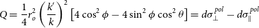
 \begin{equation} \frac{d\sigma}{d\Omega} = \frac{1}{4}r_o^2\left(\frac{k^{\prime}}{k}\right)^2\left[\frac{k}{k^{\prime}}+\frac{k^{\prime}}{k}-2+4 \cos^2\Theta \right]\end{equation}
Here, $k=\frac{h\nu}{c}$
is the incident photon momentum,
$k=\frac{h\nu}{c}$
is the incident photon momentum, $k^{\prime}=\frac{h\nu'}{c}$
is the scattered photon momentum,
$k^{\prime}=\frac{h\nu'}{c}$
is the scattered photon momentum, $\nu$
and
$\nu$
and $\nu'$
are incident and scattered photon frequency, h is the plank constant, c is the speed of light,
$\nu'$
are incident and scattered photon frequency, h is the plank constant, c is the speed of light, $\Theta$
is the angle between electric vector of scattered (
$\Theta$
is the angle between electric vector of scattered ( $k^{\prime}_{e}$
) and incident (
$k^{\prime}_{e}$
) and incident ( $k_e$
) photon,
$k_e$
) photon, $r_o = \frac{e^2}{mc^2}$
is the classical radius of the electron, e is the elementary charge, m is the mass of the electron, and
$r_o = \frac{e^2}{mc^2}$
is the classical radius of the electron, e is the elementary charge, m is the mass of the electron, and $d\Omega$
is the differential element of solid angle. The angle
$d\Omega$
is the differential element of solid angle. The angle $\Theta$
can be determined in terms of angle made by respective electric vectors with (k
$\Theta$
can be determined in terms of angle made by respective electric vectors with (k $\times$
k
′)-axis (or perpendicular direction to the scattering plane) as, see Fig. 1,
$\times$
k
′)-axis (or perpendicular direction to the scattering plane) as, see Fig. 1,
 \begin{equation} \cos \Theta = \cos\theta_e \cos\theta'_{\!\!e} + \sin\theta_e \sin\theta'_{\!\!e} \cos\!(\phi_e-\phi'_{\!\!e})\end{equation}
Here, $\theta_e$
and
$\theta_e$
and $\theta'_{\!\!e}$
are the
$\theta'_{\!\!e}$
are the $\theta$
-angle of electric vector of incident and scattered photon with (k
$\theta$
-angle of electric vector of incident and scattered photon with (k $\times$
k
′) direction (which acts as a z-axis), respectively; and
$\times$
k
′) direction (which acts as a z-axis), respectively; and $\phi_e$
and
$\phi_e$
and $\phi'_{\!\!e}$
are corresponding
$\phi'_{\!\!e}$
are corresponding $\phi$
-angles, which are related to the scattering angle
$\phi$
-angles, which are related to the scattering angle $\theta$
as
$\theta$
as $\phi_e - \phi'_{\!\!e}$ $\equiv$ $\pm \pi + \theta$
. The scattered frequency is determined in electron rest frame as
$\pm \pi + \theta$
. The scattered frequency is determined in electron rest frame as
 \begin{equation} \frac{\nu'}{\nu} = \frac{1}{1+\frac{h\nu}{m_e c^2} (1-\cos \theta)}\end{equation}
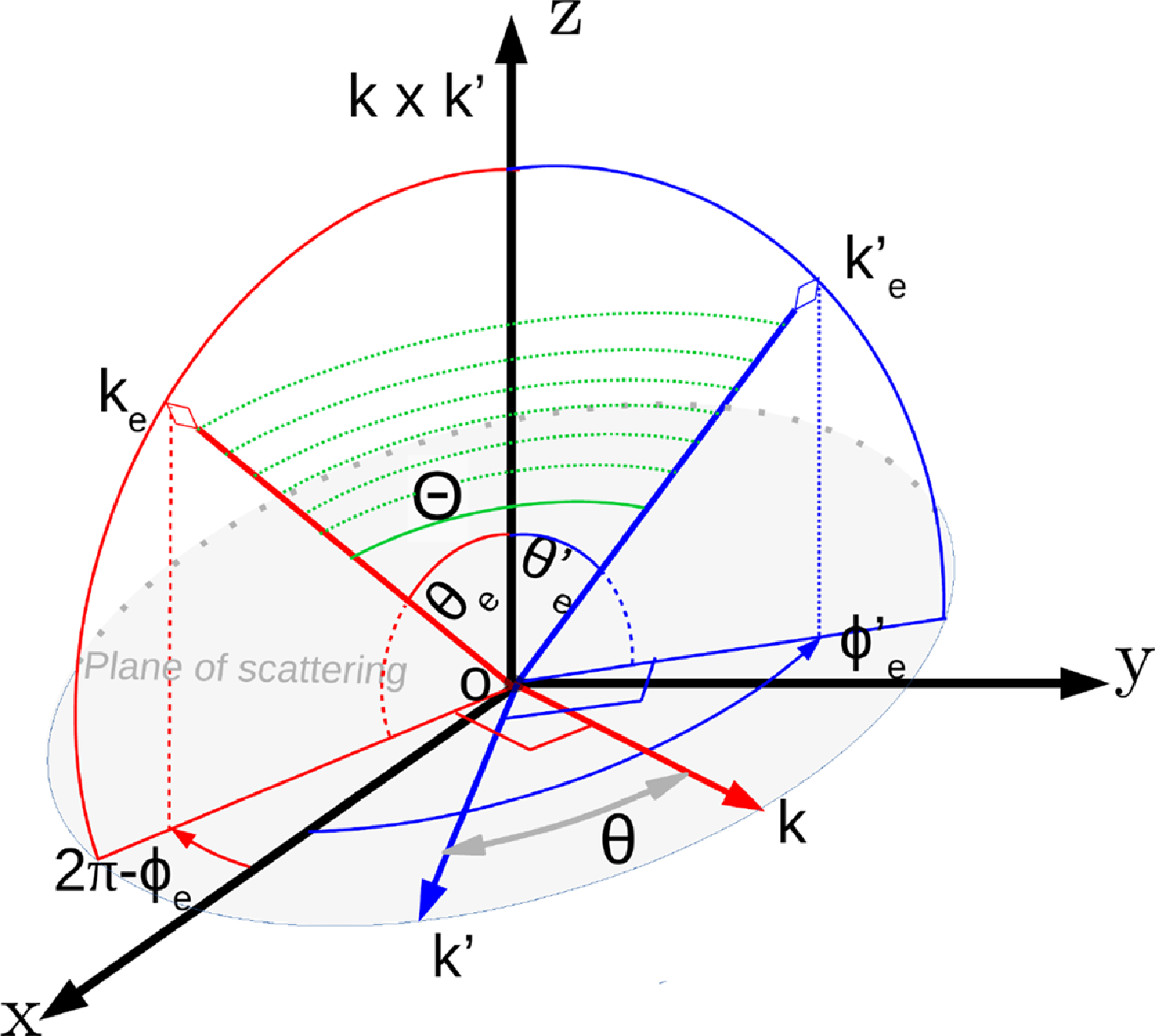
Figure 1. A schematic diagram for computation in local ( $k \times k^{\prime}$
) coordinate where the (
$k \times k^{\prime}$
) coordinate where the ( $k \times k^{\prime}$
) acts as z-axis. In this coordinate the (x,y)-plane is a scattering plane, shown by the gray area. The perpendicular plane to k is a red quarter circle (or, plane containing
$k \times k^{\prime}$
) acts as z-axis. In this coordinate the (x,y)-plane is a scattering plane, shown by the gray area. The perpendicular plane to k is a red quarter circle (or, plane containing $k_e$
and
$k_e$
and $(k \times k^{\prime})$
), and the blue quarter circle is a perpendicular plane of k
′ (or, plane containing
$(k \times k^{\prime})$
), and the blue quarter circle is a perpendicular plane of k
′ (or, plane containing $k^{\prime}_{e}$
and
$k^{\prime}_{e}$
and $(k \times k^{\prime})$
). The polarisation angle is
$(k \times k^{\prime})$
). The polarisation angle is $\theta_e$
and
$\theta_e$
and $\theta'_{\!\!e}$
for k and k
′, respectively, and measured with respect to
$\theta'_{\!\!e}$
for k and k
′, respectively, and measured with respect to $(k \times k^{\prime})$
. The
$(k \times k^{\prime})$
. The $\Theta$
is the angle between
$\Theta$
is the angle between $k_e$
and
$k_e$
and $k^{\prime}_{e}$
, the plane containing
$k^{\prime}_{e}$
, the plane containing $k_e$
and
$k_e$
and $k^{\prime}_{e}$
is shown by the green dotted lines. The direction of
$k^{\prime}_{e}$
is shown by the green dotted lines. The direction of $k_e$
and
$k_e$
and $k^{\prime}_{e}$
are
$k^{\prime}_{e}$
are $(\theta_e, \phi_e)$
and
$(\theta_e, \phi_e)$
and $(\theta'_{\!\!e}, \phi'_{\!\!e})$
, respectively; thus, the scattering angle
$(\theta'_{\!\!e}, \phi'_{\!\!e})$
, respectively; thus, the scattering angle $\theta$
is
$\theta$
is $\theta$
=
$\theta$
= $(\phi_e-\phi'_{\!\!e})-\pi$
.
$(\phi_e-\phi'_{\!\!e})-\pi$
.
The polarised radiation is uniquely described by four Stokes parameters, I, Q, U, and V, with constraint $I = \sqrt{Q^2 + U^2 + V^2}$
. It is defined as
$I = \sqrt{Q^2 + U^2 + V^2}$
. It is defined as $I \equiv I_x + I_y$
;
$I \equiv I_x + I_y$
; $Q \equiv I_x - I_y$
;
$Q \equiv I_x - I_y$
; $U \equiv I_{x+45}-I_{y+45}$
, and V is a measured of the circular polarisation, thus for the present study
$U \equiv I_{x+45}-I_{y+45}$
, and V is a measured of the circular polarisation, thus for the present study $V = 0$
. Here,
$V = 0$
. Here, $I_x, I_y$
are the intensity measured along the one of polarised direction, say, along the x-axis and perpendicular to it (or along the y-axis, as here we assume that the photon is travelling along the z-axis);
$I_x, I_y$
are the intensity measured along the one of polarised direction, say, along the x-axis and perpendicular to it (or along the y-axis, as here we assume that the photon is travelling along the z-axis); $I_{x+45}, I_{y+45}$
are the intensity measured along the direction which obtains by rotating the x- and y-axis with 45 degree, respectively. The degree of polarisation P and the angle of polarisation
$I_{x+45}, I_{y+45}$
are the intensity measured along the direction which obtains by rotating the x- and y-axis with 45 degree, respectively. The degree of polarisation P and the angle of polarisation $\chi$
are defined as (e.g. Lei et al. Reference Lei, Dean and Hills1997; Bonometto, Cazzola, & Saggion Reference Bonometto, Cazzola and Saggion1970)
$\chi$
are defined as (e.g. Lei et al. Reference Lei, Dean and Hills1997; Bonometto, Cazzola, & Saggion Reference Bonometto, Cazzola and Saggion1970)
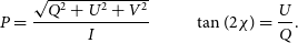 \begin{equation} P = \frac{\sqrt{Q^2+U^2+V^2}}{I} \quad \ \ \quad \tan (2\chi) = \frac{U}{Q}.\end{equation}
For an unpolarised radiation, P = 0, as $I_x = I_y = I_{x+45} = I_{y+45}$
. For a partially polarised radiation, and
$I_x = I_y = I_{x+45} = I_{y+45}$
. For a partially polarised radiation, and $P = Q/I$
, the P varies from −1 to 1, here
$P = Q/I$
, the P varies from −1 to 1, here $P = 1$
is for the completely polarised radiation with electric vector along the x-axis and
$P = 1$
is for the completely polarised radiation with electric vector along the x-axis and $P = -1$
is for the electric vector along the y-axis.
$P = -1$
is for the electric vector along the y-axis.
In Compton scattering, to define the Stokes parameters, customary we choose one linear polarisation direction is perpendicular to the plane of scattering (or along the ( $k \times k^{\prime}$
) direction) and another one is parallel to the scattering plane (i.e. the electric vector of scattered/ incident photon lies on the scattering plane) and the corresponding measured intensity is denoted in terms of differential cross section by
$k \times k^{\prime}$
) direction) and another one is parallel to the scattering plane (i.e. the electric vector of scattered/ incident photon lies on the scattering plane) and the corresponding measured intensity is denoted in terms of differential cross section by $\sigma_\perp$
(
$\sigma_\perp$
( $I_\perp)$
and
$I_\perp)$
and $\sigma_\parallel$
(
$\sigma_\parallel$
( $I_\parallel$
), respectively. In present notation, the
$I_\parallel$
), respectively. In present notation, the $\theta'_{\!\!e}$
= 0 and
$\theta'_{\!\!e}$
= 0 and $\pi/2$
for
$\pi/2$
for $\sigma_\perp$
and
$\sigma_\perp$
and $\sigma_\parallel$
, respectively. Since, for unpolarised electrons, we have one of Stokes parameter
$\sigma_\parallel$
, respectively. Since, for unpolarised electrons, we have one of Stokes parameter $V = 0$
, also in next section we will show that either U = 0 (for unpolarised incident photons) or
$V = 0$
, also in next section we will show that either U = 0 (for unpolarised incident photons) or $U \ll Q$
(for polarised low-energy incident photons). Therefore, in general, for the partial polarised photons (a mixture of polarised and unpolarised photons) the degree of polarisation for Compton scattering with unpolarised electrons can be written as (e.g. Lei et al. Reference Lei, Dean and Hills1997; Dolan Reference Dolan1967)
$U \ll Q$
(for polarised low-energy incident photons). Therefore, in general, for the partial polarised photons (a mixture of polarised and unpolarised photons) the degree of polarisation for Compton scattering with unpolarised electrons can be written as (e.g. Lei et al. Reference Lei, Dean and Hills1997; Dolan Reference Dolan1967)
 \begin{equation} P = \frac{Q}{I} = \frac{I_\perp - I_\parallel}{I_\perp + I_\parallel} = \frac{\sigma_\perp - \sigma_\parallel}{\sigma_\perp + \sigma_\parallel}\end{equation}
The angle of polarisation $\chi$
of the scattered photons also measures the angle between two consecutive scattering planes (e.g. McMaster Reference McMaster1961). In other words, the angle between
$\chi$
of the scattered photons also measures the angle between two consecutive scattering planes (e.g. McMaster Reference McMaster1961). In other words, the angle between $(k \times k^{\prime})$
and
$(k \times k^{\prime})$
and $(k \times k^{\prime})_{next}$
is
$(k \times k^{\prime})_{next}$
is $\chi$
. Since, the
$\chi$
. Since, the $k^{\prime}_{e}$
,
$k^{\prime}_{e}$
, $(k \times k^{\prime})$
and
$(k \times k^{\prime})$
and $(k \times k^{\prime})_{next}$
all are lied in perpendicular plane to k
′, therefore for next scattering:
$(k \times k^{\prime})_{next}$
all are lied in perpendicular plane to k
′, therefore for next scattering:
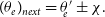 \begin{equation} (\theta_e)_{next} = \theta'_{\!\!e} \pm \chi. \end{equation}
However for incident photons, there is no information of previous scattering, only one has k and $k_e$
. In computation, for first scattering one has to define the scattering plane freshly, without loss of generality we assume that the angle of polarisation (
$k_e$
. In computation, for first scattering one has to define the scattering plane freshly, without loss of generality we assume that the angle of polarisation ( $\chi_{previous}$
) of incident photons is
$\chi_{previous}$
) of incident photons is $\theta_e$
with considering
$\theta_e$
with considering $(\theta'_{\!\!e})_{previous}$
= 0. Here, the subscript previous and next is used for the quantity related to the previous and next scattering, respectively. For clarity, we denote the angle of polarisation of the incident photons by
$(\theta'_{\!\!e})_{previous}$
= 0. Here, the subscript previous and next is used for the quantity related to the previous and next scattering, respectively. For clarity, we denote the angle of polarisation of the incident photons by $\phi$
.
$\phi$
.
2.1. Compton scattering of unpolarised photons
For an unpolarised incident photons, the $\sigma_\perp$
and
$\sigma_\perp$
and $\sigma_\parallel$
can be determined by averaging the
$\sigma_\parallel$
can be determined by averaging the $\cos^2\Theta$
-term of equation (1) over
$\cos^2\Theta$
-term of equation (1) over $\theta_e$
using equation (2) for
$\theta_e$
using equation (2) for $\theta'_{\!\!e}$
= 0 and
$\theta'_{\!\!e}$
= 0 and $\pi/2$
, respectively, and it is expressed as (see, e.g. McMaster Reference McMaster1961):
$\pi/2$
, respectively, and it is expressed as (see, e.g. McMaster Reference McMaster1961):
 \begin{align*} d\sigma_\perp^{unpol} = \frac{1}{4}r_o^2\left(\frac{k^{\prime}}{k}\right)^2\left[\frac{k}{k^{\prime}}+\frac{k^{\prime}}{k}\right], \end{align*}
 \begin{align*}d\sigma_\parallel^{unpol} = \frac{1}{4}r_o^2\left(\frac{k^{\prime}}{k}\right)^2\left[\frac{k}{k^{\prime}}+\frac{k^{\prime}}{k}-2\sin^2\theta\right], \end{align*}
here, $\langle \cos^2\theta_e\rangle$
=
$\langle \cos^2\theta_e\rangle$
= $\langle \sin^2\theta_e\rangle$
=0.5; and
$\langle \sin^2\theta_e\rangle$
=0.5; and $\langle \cos\theta_e\rangle$
=
$\langle \cos\theta_e\rangle$
= $\langle \sin\theta_e\rangle$
=0, as for the unpolarised photons the
$\langle \sin\theta_e\rangle$
=0, as for the unpolarised photons the $\theta_e$
is distributed isotropically.
$\theta_e$
is distributed isotropically.
The angle of polarisation: Similarly, we estimate the $\sigma_{\perp+45}^{unpol}$
and
$\sigma_{\perp+45}^{unpol}$
and $\sigma_{\parallel+45}^{unpol}$
with having
$\sigma_{\parallel+45}^{unpol}$
with having $\theta'_{\!\!e}$
=
$\theta'_{\!\!e}$
= $\pi/4$
and
$\pi/4$
and $3\pi/4$
, respectively, its values are
$3\pi/4$
, respectively, its values are $\sigma_{\perp+45}^{unpol} = \sigma_{\parallel+45}^{unpol} = \frac{1}{4}r_o^2\left(\frac{k^{\prime}}{k}\right)^2\left[\frac{k}{k^{\prime}}+\frac{k^{\prime}}{k}-\sin^2\theta\right]$
. Thus, the Stokes parameter U is zero, which gives
$\sigma_{\perp+45}^{unpol} = \sigma_{\parallel+45}^{unpol} = \frac{1}{4}r_o^2\left(\frac{k^{\prime}}{k}\right)^2\left[\frac{k}{k^{\prime}}+\frac{k^{\prime}}{k}-\sin^2\theta\right]$
. Thus, the Stokes parameter U is zero, which gives $\chi = 0$
. Therefore, after single scattering, the scattered photons are polarised along the
$\chi = 0$
. Therefore, after single scattering, the scattered photons are polarised along the $(k \times k^{\prime})$
direction or in another words, the plane of polarisation of scattered photons is along the perpendicular to the scattering plane.
$(k \times k^{\prime})$
direction or in another words, the plane of polarisation of scattered photons is along the perpendicular to the scattering plane.
The degree of polarisation: The degree of linear polarisation of the scattered photons after single scattering of unpolarised photons is written (using equation (5)) as (see, e.g. McMaster Reference McMaster1961; Matt et al. Reference Matt, Feroci, Rapisarda and Costa1996; Lei et al. Reference Lei, Dean and Hills1997):
 \begin{equation} P = \frac{\sin^2\theta}{\frac{k}{k^{\prime}}+\frac{k^{\prime}}{k}-\sin^2\theta}.\end{equation}
Here, P = 0, for $\theta$
= 0, and
$\theta$
= 0, and $P = \frac{1}{\frac{k}{k^{\prime}}+\frac{k^{\prime}}{k}-1}$
for
$P = \frac{1}{\frac{k}{k^{\prime}}+\frac{k^{\prime}}{k}-1}$
for $\theta$
= 90
$\theta$
= 90 $^{\circ}$
. In Thomson limit (precisely defined as
$^{\circ}$
. In Thomson limit (precisely defined as $\frac{h\nu}{\gamma \ m_e c^2} \ll 1$
, here
$\frac{h\nu}{\gamma \ m_e c^2} \ll 1$
, here $\gamma = 1/\sqrt{(1 - \frac{\text v^2}{c^2})}$
is the electrons Lorentz factor,
$\gamma = 1/\sqrt{(1 - \frac{\text v^2}{c^2})}$
is the electrons Lorentz factor, $\text v$
is the speed of electron), one has
$\text v$
is the speed of electron), one has $\frac{k}{k^{\prime}} \sim 1$
(see equation (3)), thus P = 1 for
$\frac{k}{k^{\prime}} \sim 1$
(see equation (3)), thus P = 1 for $\theta = 90^{\circ}$
. Hence, in Thomson regime the single scattered unpolarised (incident) photons at
$\theta = 90^{\circ}$
. Hence, in Thomson regime the single scattered unpolarised (incident) photons at $\theta =90^{\circ}$
are completely polarised in a perpendicular plane to the scattering plane.
$\theta =90^{\circ}$
are completely polarised in a perpendicular plane to the scattering plane.
Modulation curve: The modulation curve is a distribution of the $(\theta'_{\!\!e})$
-angle. The differential cross section for unpolarised incident photons can be expressed by using equations (1) and (2) as:
$(\theta'_{\!\!e})$
-angle. The differential cross section for unpolarised incident photons can be expressed by using equations (1) and (2) as:
 \begin{align*}d\sigma = \frac{1}{4}r_o^2\left(\frac{k^{\prime}}{k}\right)^2\left[\frac{k}{k^{\prime}}+\frac{k^{\prime}}{k}- 2\sin^2\theta \sin^2\theta'_{\!\!e}\right],\end{align*}
here, we consider once again $\langle \cos^2\theta_e\rangle$
=
$\langle \cos^2\theta_e\rangle$
= $\langle \sin^2\theta_e\rangle$
=0.5, and
$\langle \sin^2\theta_e\rangle$
=0.5, and $\langle \cos\theta_e\rangle$
=
$\langle \cos\theta_e\rangle$
= $\langle \sin\theta_e\rangle$
=0. The above expression after rearranging the term can be written as (using,
$\langle \sin\theta_e\rangle$
=0. The above expression after rearranging the term can be written as (using, $\cos 2\theta'_{\!\!e} = 1 -2\sin^2\theta'_{\!\!e})$
 \begin{equation} d\sigma =\frac{1}{4}r_o^2\left(\frac{k^{\prime}}{k}\right)^2\left[\frac{k}{k^{\prime}}+\frac{k^{\prime}}{k}-\sin^2\theta \right] (1 + P \cos 2\theta'_{\!\!e})\end{equation}
By comparison to the above expressed modulation curve from the commonly used expression for modulation curve in literature (e.g. equation (4.10) of Lei et al. Reference Lei, Dean and Hills1997, or, equation (2) of Chattopadhyay et al. Reference Chattopadhyay, Vadawale, Rao, Sreekumar and Bhattacharya2014, note there, authors have measured the corresponding $\theta'_{\!\!e}$
with respect to the scattering plane), we again find that the angle of polarisation for scattered photons after single scattering of unpolarised incident photons is zero, that is, the linear polarisation is along the perpendicular direction to the scattering plane.
$\theta'_{\!\!e}$
with respect to the scattering plane), we again find that the angle of polarisation for scattered photons after single scattering of unpolarised incident photons is zero, that is, the linear polarisation is along the perpendicular direction to the scattering plane.
For polarisation-insensitive detector: The cross section for a polarisation-insensitive detector can be written (by using equations (1) and (2), and now with having additional $\langle \cos^2\theta'_{\!\!e}\rangle$
=
$\langle \cos^2\theta'_{\!\!e}\rangle$
= $\langle \sin^2\theta'_{\!\!e}\rangle$
=0.5) as:
$\langle \sin^2\theta'_{\!\!e}\rangle$
=0.5) as:
 \begin{equation} d\sigma_{ins-detct} = \frac{1}{4}r_o^2\left(\frac{k^{\prime}}{k}\right)^2\left[\frac{k}{k^{\prime}}+\frac{k^{\prime}}{k}-\sin^2\theta\right]\end{equation}
Also, here $d\sigma_{ins-detct} = (d\sigma_\perp^{unpol} + d\sigma_\parallel^{unpol})/2 = (d\sigma_{\perp+45}^{unpol} + d\sigma_{\parallel+45}^{unpol})/2 $
.
$d\sigma_{ins-detct} = (d\sigma_\perp^{unpol} + d\sigma_\parallel^{unpol})/2 = (d\sigma_{\perp+45}^{unpol} + d\sigma_{\parallel+45}^{unpol})/2 $
.
2.2. Compton scattering of polarised photons
For a completely polarised incident photons with polarisation angle $\phi$
(i.e.
$\phi$
(i.e. $\theta_e = \phi$
) the cross section can be obtained by averaging the equation (1) over
$\theta_e = \phi$
) the cross section can be obtained by averaging the equation (1) over $\theta'_{\!\!e}$
(see, e.g. Lei et al. Reference Lei, Dean and Hills1997, and reference therein), and it is written as:
$\theta'_{\!\!e}$
(see, e.g. Lei et al. Reference Lei, Dean and Hills1997, and reference therein), and it is written as:
 \begin{equation} \frac{d\sigma}{d\Omega}^{pol} = \frac{1}{4}r_o^2\left(\frac{k^{\prime}}{k}\right)^2\left[\frac{k}{k^{\prime}}+\frac{k^{\prime}}{k}-2\sin^2\phi \sin^2\theta \right],\end{equation}
here we consider $\langle \cos^2\theta'_{\!\!e}\rangle$
=
$\langle \cos^2\theta'_{\!\!e}\rangle$
= $\langle \sin^2\theta'_{\!\!e}\rangle$
= 0.5, and
$\langle \sin^2\theta'_{\!\!e}\rangle$
= 0.5, and $\langle \cos\theta_e\rangle$
=
$\langle \cos\theta_e\rangle$
= $\langle \sin\theta_e\rangle$
= 0. However, it is expected that the distribution of
$\langle \sin\theta_e\rangle$
= 0. However, it is expected that the distribution of $\theta'_{\!\!e}$
is no longer isotropic but depends on the cross section, equation (1) (see, e.g. Matt et al. Reference Matt, Feroci, Rapisarda and Costa1996). Similar to the unpolarised incident photons case, we compute the
$\theta'_{\!\!e}$
is no longer isotropic but depends on the cross section, equation (1) (see, e.g. Matt et al. Reference Matt, Feroci, Rapisarda and Costa1996). Similar to the unpolarised incident photons case, we compute the $d\sigma_\perp$
and
$d\sigma_\perp$
and $d\sigma_\parallel$
for polarised incident photons with having
$d\sigma_\parallel$
for polarised incident photons with having $\theta'_{\!\!e}$
= 0 and
$\theta'_{\!\!e}$
= 0 and $\pi/2$
, respectively, which is written as (see, e.g. McMaster Reference McMaster1961):
$\pi/2$
, respectively, which is written as (see, e.g. McMaster Reference McMaster1961):
 \begin{align*}\begin{aligned}d\sigma_\perp^{pol} =\frac{1}{4}r_o^2\left(\frac{k^{\prime}}{k}\right)^2\left[\frac{k}{k^{\prime}}+\frac{k^{\prime}}{k}-2+4 \cos^2\phi \right]\\[5pt] d\sigma_\parallel^{pol}=\frac{1}{4}r_o^2\left(\frac{k^{\prime}}{k}\right)^2\left[\frac{k}{k^{\prime}}+\frac{k^{\prime}}{k}-2+ 4\sin^2\phi \cos^2\theta \right]\end{aligned}\end{align*}
The angle of polarisation: The $d\sigma_{\perp+45}$
and
$d\sigma_{\perp+45}$
and $d\sigma_{\parallel+45}$
for polarised incident photons are
$d\sigma_{\parallel+45}$
for polarised incident photons are $d\sigma_{\perp+45}^{pol} = \frac{1}{4}r_o^2\left(\frac{k^{\prime}}{k}\right)^2\left[\frac{k}{k^{\prime}}+\frac{k^{\prime}}{k}-2+2(\cos^2\phi +\sin^2\phi\cos^2\theta +\sin2\phi \cos\theta) \right]$
, and
$d\sigma_{\perp+45}^{pol} = \frac{1}{4}r_o^2\left(\frac{k^{\prime}}{k}\right)^2\left[\frac{k}{k^{\prime}}+\frac{k^{\prime}}{k}-2+2(\cos^2\phi +\sin^2\phi\cos^2\theta +\sin2\phi \cos\theta) \right]$
, and $d\sigma_{\parallel+45}^{pol} = \frac{1}{4}r_o^2\left(\frac{k^{\prime}}{k}\right)^2[\frac{k}{k^{\prime}}+\frac{k^{\prime}}{k}-2+2(\cos^2\phi +\sin^2\phi\cos^2\theta -$ $\sin2\phi \cos\theta) ]$
. Here,
$\sin2\phi \cos\theta) ]$
. Here, $\theta'_{\!\!e}$
=
$\theta'_{\!\!e}$
= $\pi/4$
and
$\pi/4$
and $3\pi/4$
for
$3\pi/4$
for $d\sigma_{\perp+45}^{pol}$
and
$d\sigma_{\perp+45}^{pol}$
and $d\sigma_{\parallel+45}^{pol}$
, respectively. The Stokes parameters U
$d\sigma_{\parallel+45}^{pol}$
, respectively. The Stokes parameters U $\&$
Q are expressed as:
$\&$
Q are expressed as:
 \begin{align*} U = \frac{1}{4}r_o^2\left(\frac{k^{\prime}}{k}\right)^2\left[4\sin2\phi \cos\theta) \right] =d\sigma_{\perp+45}^{pol} - d\sigma_{\parallel+45}^{pol} \end{align*}
 \begin{align*} Q = \frac{1}{4}r_o^2\left(\frac{k^{\prime}}{k}\right)^2\left[4\cos^2\phi-4\sin^2\phi\cos^2\theta\right] =d\sigma_{\perp}^{pol} - d\sigma_{\parallel}^{pol}\end{align*}
The angle of polarisation can be obtained by using expression (4). In practice, the average angle of polarisation $\langle \chi\rangle$
is interested, it is written as (e.g. Li et al. Reference Li, Narayan and McClintock2009):
$\langle \chi\rangle$
is interested, it is written as (e.g. Li et al. Reference Li, Narayan and McClintock2009):
 \begin{equation} \tan2\langle \chi\rangle = \frac{\langle U \rangle}{\langle Q \rangle},\end{equation}
here, $\langle U \rangle$
and
$\langle U \rangle$
and $\langle Q \rangle$
are averaged of U and Q over angle, respectively. In Thomson limit, we find that the magnitude of
$\langle Q \rangle$
are averaged of U and Q over angle, respectively. In Thomson limit, we find that the magnitude of $\langle U \rangle$
is almost one order less than the magnitude of
$\langle U \rangle$
is almost one order less than the magnitude of $\langle Q \rangle$
, that is,
$\langle Q \rangle$
, that is, $|\langle U \rangle| << |\langle Q \rangle|$
. Thus,
$|\langle U \rangle| << |\langle Q \rangle|$
. Thus, $\langle \chi \rangle$ $\sim$
0 or
$\sim$
0 or $\pi/2$
for a positive or negative value of
$\pi/2$
for a positive or negative value of $\langle Q \rangle$
, respectively.
$\langle Q \rangle$
, respectively.
The degree of polarisation: On average $|\langle U \rangle| < < |\langle Q \rangle|$
, but we notice also
$|\langle U \rangle| < < |\langle Q \rangle|$
, but we notice also $U > Q$
for a range of
$U > Q$
for a range of $\theta$
, for example, see Fig. A1. Hence we define the PD with considering two extreme cases, case A:
$\theta$
, for example, see Fig. A1. Hence we define the PD with considering two extreme cases, case A: $|Q| >> |U|$
and case B:
$|Q| >> |U|$
and case B: $|Q| \sim |U|$
. For case A, the degree of polarisation for single scattered photons of polarised incident photons is expressed by using equation (5) as:
$|Q| \sim |U|$
. For case A, the degree of polarisation for single scattered photons of polarised incident photons is expressed by using equation (5) as:
 \begin{equation}P_A = \frac{Q}{I} = \frac{2 - 2\sin^2\phi(1+\cos^2\theta)}{\frac{k^{\prime}}{k}+\frac{k}{k^{\prime}}-2\sin^2\phi\sin^2\theta}\end{equation}
For case B, it is expressed by using equation (4) as (see, e.g. Matt et al. Reference Matt, Feroci, Rapisarda and Costa1996; Lei et al. Reference Lei, Dean and Hills1997):
 \begin{equation}P_B = \frac{\sqrt{Q^2+U^2}}{I} = \frac{2 - 2\sin^2\phi\sin^2\theta}{\frac{k^{\prime}}{k}+\frac{k}{k^{\prime}}-2\sin^2\phi\sin^2\theta}\end{equation}
In Thomson regime, $P_B$
= 1.
$P_B$
= 1.
Some interesting facts:
(i) $\theta$
=
0:
For
$\theta$
=
0:
For $\theta = 0$
,
$\theta = 0$
, $Q \propto \cos\!(2\phi)$
and
$Q \propto \cos\!(2\phi)$
and $U \propto \sin(2\phi)$
. Since for
$U \propto \sin(2\phi)$
. Since for $\theta=0$
one has
$\theta=0$
one has $k=k^{\prime}$
which gives
$k=k^{\prime}$
which gives $P_B$
= 1 for all
$P_B$
= 1 for all $\phi$
. However, U = 0 for
$\phi$
. However, U = 0 for $\phi = 0, \pi/2, \pi$
, and in this case PD would be determined by
$\phi = 0, \pi/2, \pi$
, and in this case PD would be determined by $P_A$
. Here,
$P_A$
. Here, $P_A$
= 1 for
$P_A$
= 1 for $\phi = 0, \pi$
, and
$\phi = 0, \pi$
, and $P_A$
= −1 for
$P_A$
= −1 for $\phi = \pi/2$
. Conclusively,
$\phi = \pi/2$
. Conclusively, $|P|$
= 1 for
$|P|$
= 1 for $\theta = 0$
.
(ii)
$\theta = 0$
.
(ii) $\phi$
=
0
,
$\phi$
=
0
, $\pi/2$
:
For
$\pi/2$
:
For $\phi$
= 0 or
$\phi$
= 0 or $\pi/2$
,
$\pi/2$
, $U = 0$
. The PD is
$U = 0$
. The PD is $P_A = \frac{2}{\frac{k}{k^{\prime}}+\frac{k^{\prime}}{k}}$
and
$P_A = \frac{2}{\frac{k}{k^{\prime}}+\frac{k^{\prime}}{k}}$
and $\frac{-2\cos^2\theta}{\frac{k}{k^{\prime}}+\frac{k^{\prime}}{k}-2\sin^2\theta}$
for
$\frac{-2\cos^2\theta}{\frac{k}{k^{\prime}}+\frac{k^{\prime}}{k}-2\sin^2\theta}$
for $\phi$
= 0 and
$\phi$
= 0 and $\pi/2$
, respectively (for
$\pi/2$
, respectively (for $\phi =0$
, see McMaster Reference McMaster1961). In Thomson limit,
$\phi =0$
, see McMaster Reference McMaster1961). In Thomson limit, $P_A $
= 1 and −1;
$P_A $
= 1 and −1; $\chi$
= 0 and
$\chi$
= 0 and $\pi/2$
for
$\pi/2$
for $\phi = 0$
and
$\phi = 0$
and $\pi/2$
, respectively (see also Fig. 5), also by definition of Q, here
$\pi/2$
, respectively (see also Fig. 5), also by definition of Q, here $\theta'_{\!\!e}$
= 0 and
$\theta'_{\!\!e}$
= 0 and $\pi/2$
, respectively. And in words, the polarisation properties of scattered photons are same to the incident photons.
(iii)
$\pi/2$
, respectively. And in words, the polarisation properties of scattered photons are same to the incident photons.
(iii) $\phi$
=
$\phi$
= $\pi$
/4:
For
$\pi$
/4:
For $\phi = \pi/4$
, it is expected that the incident polarised photons behave like unpolarised photons. It means that the degree of polarisation of scattered photons will be described by expression (7). We note that for
$\phi = \pi/4$
, it is expected that the incident polarised photons behave like unpolarised photons. It means that the degree of polarisation of scattered photons will be described by expression (7). We note that for $\phi = \pi/4$
the only
$\phi = \pi/4$
the only $P_A$
reduces to the expression (7).
$P_A$
reduces to the expression (7).
Modulation curve: The expression for modulation curve is written by using equation (1) as:
 \begin{align} \frac{d\sigma}{d\Omega}^{pol} &= \frac{1}{4}r_o^2\left(\frac{k^{\prime}}{k}\right)^2\left[\frac{k}{k^{\prime}}+\frac{k^{\prime}}{k}-2 + 4(\cos^2\phi \cos^2\theta'_{\!\!e} \right. \nonumber \\[5pt] & \quad \left. + \sin^2\phi \sin^2\theta'_{\!\!e} \cos^2\theta - \frac{1}{2}\sin2\phi\sin2\theta'_{\!\!e} \cos\theta) \right].\end{align}
After rearranging the term, the above equation can be written as:
 \begin{align*}\frac{d\sigma}{d\Omega}^{pol} = \frac{1}{4}r_o^2\left(\frac{k^{\prime}}{k}\right)^2& \left[\frac{k}{k^{\prime}}+\frac{k^{\prime}}{k}-2\sin^2\phi \sin^2\theta \right] \left[1 + P_A \left(\cos2\theta'_{\!\!e} \right. \right. \nonumber \\[5pt] & \left. \left. - \frac{\sin 2\phi \cos\theta}{\cos^2\phi-2\sin^2\phi\cos^2\theta} \sin 2\theta'_{\!\!e} \right)\right]\end{align*}
2.3. A special case for polarisation measurement at $\theta$
= 0
$\theta$
= 0

For $\theta$
= 0, the cross section (1) can be written simply as:
$\theta$
= 0, the cross section (1) can be written simply as:
 \begin{equation} \frac{d\sigma}{d\Omega} = r_o^2 \cos^2(\theta_e+\theta'_{\!\!e}),\end{equation}
here we use $\frac{k^{\prime}}{k} = 1$
, for
$\frac{k^{\prime}}{k} = 1$
, for $\theta$
= 0, which is true for a electron is in either rest or motion. In this case,
$\theta$
= 0, which is true for a electron is in either rest or motion. In this case, $k^{\prime}_{e}$
will also lie on the perpendicular plane to the k, and thus for a plane the solid angle becomes
$k^{\prime}_{e}$
will also lie on the perpendicular plane to the k, and thus for a plane the solid angle becomes $d\Omega$
=
$d\Omega$
= $d\theta'_{\!\!e}$
. Hence,
$d\theta'_{\!\!e}$
. Hence, $d\sigma$ $\propto$ $\cos^2(\theta_e+\theta'_{\!\!e}) d\theta'_{\!\!e}$
, which has properties that the distribution of
$\cos^2(\theta_e+\theta'_{\!\!e}) d\theta'_{\!\!e}$
, which has properties that the distribution of $\theta'_{\!\!e}$
replicates the polarised distribution of
$\theta'_{\!\!e}$
replicates the polarised distribution of $\theta_e$
. It can be understood as (i) for unpolarised incident photons,
$\theta_e$
. It can be understood as (i) for unpolarised incident photons, $\theta_e$
is isotropically distributed; thus, the averaged cross section over
$\theta_e$
is isotropically distributed; thus, the averaged cross section over $\theta_e$
for
$\theta_e$
for $\theta'_{\!\!e}$
is simply a constant, or
$\theta'_{\!\!e}$
is simply a constant, or
 \begin{align*}\frac{d\sigma}{d\theta'_{\!\!e}} = constant. \end{align*}
(ii) for polarised incident photons, $\theta_e$
= constant =
$\theta_e$
= constant = $\phi$
, and the cross section becomes
$\phi$
, and the cross section becomes
 \begin{align*}\frac{d\sigma}{d\theta'_{\!\!e}} = r_o^2 \cos^2(\theta'_{\!\!e}+\phi) = \frac{r_o^2}{2} \left(1 + \cos\!(2(\theta'_{\!\!e}+\phi))\right),\end{align*}
which is a modulation curve for the scattered photons with degree of polarisation P = 1 and the angle of polarisation $\chi = \phi$
.
$\chi = \phi$
.
In general for the partially polarised incident photons, in which P fraction is the polarised photons with polarisation angle $\phi$
and
$\phi$
and $(1-P)$
fraction is the unpolarised photons, the modulation curve can be written as:
$(1-P)$
fraction is the unpolarised photons, the modulation curve can be written as:
 \begin{equation} \frac{d\sigma}{d\theta'_{\!\!e}} = A + B \cos\!(2(\theta'_{\!\!e}+\phi))\end{equation}
here, A and B are a normalisation factor, and clearly, $P = B/A$
and
$P = B/A$
and $\chi = \phi$
. The above expression is similar to the equation (4.10) of Lei et al. (Reference Lei, Dean and Hills1997).
$\chi = \phi$
. The above expression is similar to the equation (4.10) of Lei et al. (Reference Lei, Dean and Hills1997).
2.4. Lorentz invariance of the Stokes parameters
We know that the field of the radiation is transverse in any reference frame, and the Lorentz boost subjects to an aberration effect of radiation. Since the electric vector always lies on the perpendicular plane to radiation propagation direction, and these electric vectors will be transformed from one frame to another Lorentz-boosted frame with the same rule. Thus, if the radiation is completely polarised in one reference frame, then it will be completely polarised in any Lorentz-boosted frame. In other words, the degree of polarisation of photons in any Lorentz-boosted frame is same to the magnitude of PD in the electron rest frame. Later, we will argue that in Compton scattering the angle of polarisation for photons remains the same in any Lorentz-boosted frame. Hence, the Stokes parameters are invariant under Lorentz transformations (see, e.g. Landau & Lifshitz Reference Landau and Lifshitz1987; Krawczynski Reference Krawczynski2012, references therein).
3. Monte Carlo method
The Klein–Nishina differential cross section for unpolarised rest electrons expressed by equation (1) depends mainly on momentum of incident photon k, $\Theta$
-angle, and scattering angle
$\Theta$
-angle, and scattering angle $\theta$
. For a given incident photon direction and polarisation angle
$\theta$
. For a given incident photon direction and polarisation angle $\phi$
(=
$\phi$
(= $\theta_e$
by assumption), in principle, without affecting the cross section one can take any direction of (
$\theta_e$
by assumption), in principle, without affecting the cross section one can take any direction of ( $k \times k^{\prime}$
) on the perpendicular plane to k with maintaining the
$k \times k^{\prime}$
) on the perpendicular plane to k with maintaining the $k_e$
direction such that the angle between
$k_e$
direction such that the angle between $k_e$
and (
$k_e$
and ( $k \times k^{\prime}$
) is
$k \times k^{\prime}$
) is $\theta_e$
. Hence, for a known incident photon direction and polarisation, any scattering plane is permissible according to the cross section unless the direction of
$\theta_e$
. Hence, for a known incident photon direction and polarisation, any scattering plane is permissible according to the cross section unless the direction of $k_e$
is not fixed in space (say, global coordinate). In case of the fixed
$k_e$
is not fixed in space (say, global coordinate). In case of the fixed $k_e$
in space, the photon can scatter onto two planes only, as there are only two possible ways for the (
$k_e$
in space, the photon can scatter onto two planes only, as there are only two possible ways for the ( $k \times k^{\prime}$
) presentations, left and right side of the
$k \times k^{\prime}$
) presentations, left and right side of the $k_e$
. Next, for a known incident photon direction, polarisation angle and fixed
$k_e$
. Next, for a known incident photon direction, polarisation angle and fixed $k_e$
in space (i.e. fixed scattering plane) if the
$k_e$
in space (i.e. fixed scattering plane) if the $\Theta$
-angle is known then according to the cross section the electric vector of scattered photon
$\Theta$
-angle is known then according to the cross section the electric vector of scattered photon $k^{\prime}_{e}$
lies on the surface of cone with opening angle
$k^{\prime}_{e}$
lies on the surface of cone with opening angle $\Theta$
and cone-axis along the
$\Theta$
and cone-axis along the $k_e$
. Since, the scattering plane is fixed, so
$k_e$
. Since, the scattering plane is fixed, so $(k \times k^{\prime})$
also. And the k
′ direction can be determined in a perpendicular direction to the plane containing
$(k \times k^{\prime})$
also. And the k
′ direction can be determined in a perpendicular direction to the plane containing $k^{\prime}_{e}$
and
$k^{\prime}_{e}$
and $(k \times k^{\prime})$
, in which
$(k \times k^{\prime})$
, in which $k^{\prime}_{e}$
is any one of vectors which lies on that cone. Simply, if one takes
$k^{\prime}_{e}$
is any one of vectors which lies on that cone. Simply, if one takes $(k \times k^{\prime})$
as a z-axis then the intersection of
$(k \times k^{\prime})$
as a z-axis then the intersection of $\phi$
-plane and that cone gives
$\phi$
-plane and that cone gives $k^{\prime}_{e}$
and the normal to this
$k^{\prime}_{e}$
and the normal to this $\phi$
-plane (which cuts that cone) will give k
′ (see Fig. 1, however for clarity, the cone containing possible
$\phi$
-plane (which cuts that cone) will give k
′ (see Fig. 1, however for clarity, the cone containing possible $k^{\prime}_{e}$
is not shown). It can be understood easily when
$k^{\prime}_{e}$
is not shown). It can be understood easily when $k_e$
lies on the scattering plane (i.e. (x,y)-plane), and here one can note that for a particular value of
$k_e$
lies on the scattering plane (i.e. (x,y)-plane), and here one can note that for a particular value of $\Theta$
either some definite range of
$\Theta$
either some definite range of $\theta$
or,
$\theta$
or, $\theta'_{\!\!e}$
is possible. In another example when
$\theta'_{\!\!e}$
is possible. In another example when $k_e$
is along the (
$k_e$
is along the ( $k \times k^{\prime}$
), in this case, the photon can scatter in all possible directions of the scattering plane, and obviously
$k \times k^{\prime}$
), in this case, the photon can scatter in all possible directions of the scattering plane, and obviously $\theta'_{\!\!e} = \Theta$
. Hence, for a given polarisation characteristics of incident photon, and for given
$\theta'_{\!\!e} = \Theta$
. Hence, for a given polarisation characteristics of incident photon, and for given $\Theta$
-angle, only the definite range of
$\Theta$
-angle, only the definite range of $\theta$
and
$\theta$
and $\theta'_{\!\!e}$
is permissible, where
$\theta'_{\!\!e}$
is permissible, where $\theta$
and
$\theta$
and $\theta'_{\!\!e}$
both are related each other by equation (2).
$\theta'_{\!\!e}$
both are related each other by equation (2).
There are mainly two unknown quantities $\Theta$
-angle and scattering angle
$\Theta$
-angle and scattering angle $\theta$
for determining the Klein–Nishina cross section, as we know k and
$\theta$
for determining the Klein–Nishina cross section, as we know k and $k_e$
prior to scattering (at least, in MC calculation). But, to describe the scattered photon polarisation properties one needs the angle
$k_e$
prior to scattering (at least, in MC calculation). But, to describe the scattered photon polarisation properties one needs the angle $\theta'_{\!\!e}$
, which can be obtained by using equation (2) for a known
$\theta'_{\!\!e}$
, which can be obtained by using equation (2) for a known $\Theta$
-angle and
$\Theta$
-angle and $\theta$
. Therefore, to examine the polarisation in Compton scattering, one have three unknown quantities
$\theta$
. Therefore, to examine the polarisation in Compton scattering, one have three unknown quantities $\Theta$
-angle,
$\Theta$
-angle, $\theta$
and
$\theta$
and $\theta'_{\!\!e}$
, in which two quantities would be extracted from Klein–Nishina cross section and remaining one would be obtained by using equation (2). In above paragraph we note that in (
$\theta'_{\!\!e}$
, in which two quantities would be extracted from Klein–Nishina cross section and remaining one would be obtained by using equation (2). In above paragraph we note that in ( $k \times k^{\prime}$
)-coordinate one can easily know the possible range of
$k \times k^{\prime}$
)-coordinate one can easily know the possible range of $\theta$
(or
$\theta$
(or $\theta'_{\!\!e}$
) value for a given
$\theta'_{\!\!e}$
) value for a given $\Theta$
-angle and
$\Theta$
-angle and $k_e$
. So, it is more convincing, if one describe the Compton scattering in (
$k_e$
. So, it is more convincing, if one describe the Compton scattering in ( $k \times k^{\prime}$
) coordinate system (where the
$k \times k^{\prime}$
) coordinate system (where the $z-$
axis is along the (
$z-$
axis is along the ( $k \times k^{\prime}) $
) with expressing the cross section as a function of
$k \times k^{\prime}) $
) with expressing the cross section as a function of $\theta$
and
$\theta$
and $\theta'_{\!\!e}$
(see Fig. 1). In the present study for MC calculations, we consider the cross section, equation (1), as a function of
$\theta'_{\!\!e}$
(see Fig. 1). In the present study for MC calculations, we consider the cross section, equation (1), as a function of $\theta$
and
$\theta$
and $\theta'_{\!\!e}$
and describe the Compton scattering locally in (
$\theta'_{\!\!e}$
and describe the Compton scattering locally in ( $k \times k^{\prime}$
)-coordinate system. The algorithm for MC method is similar to the algorithm of Kumar & Misra (Reference Kumar and Misra2016b) with additional inclusion of polarisation properties. Below we have described the important steps involved in MC calculations.
$k \times k^{\prime}$
)-coordinate system. The algorithm for MC method is similar to the algorithm of Kumar & Misra (Reference Kumar and Misra2016b) with additional inclusion of polarisation properties. Below we have described the important steps involved in MC calculations.
To describe the different steps involved in MC calculations we consider, for simplicity, a spherical corona of radius L and temperature $T_e$
. The seed photon source is situated at the origin of spherical corona which illuminates in all directions. The optical depth
$T_e$
. The seed photon source is situated at the origin of spherical corona which illuminates in all directions. The optical depth $\tau$
is defined along the radial direction of the corona/medium, the electron density inside the corona is
$\tau$
is defined along the radial direction of the corona/medium, the electron density inside the corona is $n_e = \frac{\tau}{L\sigma_T}$
, where
$n_e = \frac{\tau}{L\sigma_T}$
, where $\sigma_T$
is Thomson cross section. We assume that the seed photon source is a black body with temperature
$\sigma_T$
is Thomson cross section. We assume that the seed photon source is a black body with temperature $T_b$
. We track a photon till it leaves the medium after single/multiple or zero scattering. We repeat the process for a large number of photons to make the statistics analysis.
$T_b$
. We track a photon till it leaves the medium after single/multiple or zero scattering. We repeat the process for a large number of photons to make the statistics analysis.
-
In the first step, we determine the incident photon’s energy
$E = h\nu$
from a black body distribution and the electron’s velocity from the velocity distribution of temperature
$T_e$
. We consider an isotropic distribution for the photons and electrons direction. The mean free path
$\lambda$
of photon of energy E is computed for a given
$T_e$
and
$n_e$
. We compute the above quantities in global coordinate using the scheme developed by Hua & Titarchuk (Reference Hua and Titarchuk1995) (see also Krawczynski Reference Krawczynski2012 for the polarisation scheme). -
Next, we determine the collision free path of the photon
$l_f$
in the medium with an exponential pdf (probability distribution function),
$\exp\left(\frac{-l_f}{\lambda}\right)$
, and obtain the condition for occurrence of scattering. If
$l_f > L$
then the photon escapes the medium without scattering and for
$l_f < L$
the scattering will be happened at distance
$l_f$
from the origin (or in general, from the previous site of scattering) in direction of the incident photon. -
Next, we specify the polarisation properties of the incident photon locally in
$(k\times k^{\prime})$
-coordinate of global (say, (
$k\times k^{\prime})_{\text{global}}$
-coordinate). For this we first assign the
$(k\times k^{\prime})$
direction on the perpendicular plane to k. For an unpolarised incident photon, we select the
$(k\times k^{\prime})$
direction uniformly, also
$\theta_e$
angle uniformly to determine the polarisation vector. For a polarised photon, we first fix
$k_e$
and then determine the
$(k\times k^{\prime})$
direction either left or right side of
$k_e$
at angle
$\theta_e$
on the perpendicular plane to k. -
In second step to describe the Compton scattering, we transform the quantities from global coordinate to electron rest frame.
-
– As the Stokes parameters are invariant under the Lorentz transformation, we assume that the polarisation angle also does not change. In electron rest frame, due to the aberration effect the incident photon direction will change in the plane containing
$k\ \& \ \text v$
(say,
$k_{ab}$
). Consequently, the polarisation vector will lie now in a plane perpendicular to
$k_{ab}$
, denoted as
$k_{e}^{ab}$
. The direction of
$k_{e}^{ab}$
can be determined as. Since the scattering plane is assigned in global coordinate, so to determine the scattering plane in electron rest frame, we consider an another incident photon direction on global scattering plane and transformed it into electron rest frame, thus the plane containing
$k_{ab}$
, and this transformed photon direction would be the scattering plane in electron rest frame. Therefore, (
$k\times k^{\prime}$
) in electron rest frame can be determined, and consequently one can fix the
$k_{e}^{ab}$
for a known
$\theta_e$
in this (
$k\times k^{\prime})_{\text {rest frame}}$
-coordinate. With having
$\theta'_{\!\!e}$
and
$\theta$
from the cross section in electron rest frame one can determine the scattered photon direction
$k^{\prime}_{ab}$
and its
$k_e^{'ab}$
. In a similar way, these two quantities transferred back to the (
$k\times k^{\prime})_{\text {global}}$
-coordinate. We again emphasise that one have to transform the
$k_e^{'ab}$
into
$k_e^{'}$
with the condition of
$\left. \theta'_{\!\!e} \right|_{\text{lab frame}} = \left. \theta'_{\!\!e} \right|_{\text{rest frame}}$
due to the Lorentz invariance of Stokes parameters. -
– The condition of
$\left. \theta_e \right|_{\text{lab frame}}= \left. \theta_e \right|_{\text{rest frame}}$
can be understood as. Suppose, the incident photons are fully polarised with
$\theta_e$
= 45
$^{\circ}$
. The degree of polarisation for scattered photons with almost rest electron will be described by the equation (12) for
$\phi$
=45
$^{\circ}$
(see also Fig. 5). Since the degree of polarisation is a Lorentz invariant quantity. Therefore, if these completely polarised photons scatter with moving electron then PD will still describe by equation (12) for
$\phi$
=45
$^{\circ}$
, which can be only possible when
$\left.\theta_e\right|_{lab frame} = \left. \theta_e \right|_{\textit{rest frame}}$
. Hence, in Compton scattering process the PD and
$\theta_e$
both are invariant over the Lorentz-boosted frame.
-
-
As the cross section depends only
$\theta'_{\!\!e}$
we skip the all steps which involve to determine the
$k_e^{ab}$
,
$k_e^{'ab}$
, and
$(k \times k^{\prime})_{\text{rest frame}}$
, and simply extract
$\theta$
and
$\theta'_{\!\!e}$
from the cross section in electron rest frame. -
Next, we compute the scattered photon frequency (using equation (3)), and transform back this frequency to global (lab) coordinate by computing the angle between scattered photon and incident electron. In addition, after the reverse aberration effect the scattered photon has to lie on the pre-defined scattering plane. We first compute the scattered photon’s propagation direction (k′) and polarisation vector
$k^{\prime}_{e}$
(i.e. on perpendicular plane to k’) in local
$(k\times k^{\prime})_{\text{global}}$
-coordinate and then transform back to those in the global coordinate. -
Next, we estimate the collision free distance
$l_f$
for the scattered photon (of energy
$E' = h\nu'$
) and find the distance of next site of scattering from the origin, say
$r_n$
. If
$r_n < L$
then next scattering will occur otherwise photon will escape the medium. -
For next scattering, we first determine the angle of polarisation, say
$\chi_s$
of scattered photon using equation (11). Since for double scatterings or two consecutive scatterings the angle between previous and next scattering planes is
$\chi_s$
(e.g. McMaster Reference McMaster1961), so using this we compute the
$(k \times k^{\prime})_{next}$
for next scattering on perpendicular plane to the k’. And, for a known
$k^{\prime}_{e}$
in global coordinate we compute the polarisation angle
$\theta_e$
wrt
$(k \times k^{\prime})_{next}$
. We proceed the calculations for next scattering with treating k’ of previous scattering as an incident photon, and follow the same steps until the scattered photon escapes the medium.


4. MC results verification
We verify the polarisation results of MC calculations with a theory which is revisited in Section 2, that is, for single scattering, and almost rest electron. Since, the theoretical results are derived for a given scattering plane, so in MC calculation we obtain the results without bothering about orientation of the scattering plane. However, later we consider the orientation of the scattering plane, see Section 6. In the following sections we show the MC results for polarised/unpolarised incident photons. But we will first discuss the way of computing the PD and PA for scattered photons with arbitrary scattering numbers using the results of Section 2.3.
4.1. General modulation curve to estimate the PD & PA
In Section 2.3, we showed that one can know the polarisation properties of incident photons $P \ \& \ \chi$
by mapping the distribution of
$P \ \& \ \chi$
by mapping the distribution of $\theta'_{\!\!e}$
of scattered photons at
$\theta'_{\!\!e}$
of scattered photons at $\theta$ $\sim$
0 after single scattering. In general, one can estimate the polarisation properties of scattered photons with any average scattering no., say
$\sim$
0 after single scattering. In general, one can estimate the polarisation properties of scattered photons with any average scattering no., say $\langle N_{sc} \rangle$
by mapping the distribution of
$\langle N_{sc} \rangle$
by mapping the distribution of $\theta'_{\!\!e}$
of scattered photons of
$\theta'_{\!\!e}$
of scattered photons of $\langle N_{sc} + 1 \rangle$
scattering no. at
$\langle N_{sc} + 1 \rangle$
scattering no. at $\theta$ $\sim$
0. Mathematically, we are essentially using here a probability
$\sim$
0. Mathematically, we are essentially using here a probability $\propto \cos^2(\theta_e|_{\langle N_{sc}+1\rangle} + \theta'_{\!\!e}|_{\langle N_{sc}+1\rangle})$
for constructing the distribution of
$\propto \cos^2(\theta_e|_{\langle N_{sc}+1\rangle} + \theta'_{\!\!e}|_{\langle N_{sc}+1\rangle})$
for constructing the distribution of $\theta'_{\!\!e}|_{\langle N_{sc}+1\rangle}$
for a known
$\theta'_{\!\!e}|_{\langle N_{sc}+1\rangle}$
for a known $\theta_e|_{\langle N_{sc}+1\rangle}$
(see equation (15)). From equation (6), we can write
$\theta_e|_{\langle N_{sc}+1\rangle}$
(see equation (15)). From equation (6), we can write $\theta_e|_{\langle N_{sc}+1 \rangle} = (\theta'_{\!\!e} \pm \chi)|_{\langle N_{sc}\rangle}$
, here the subscript with vertical bar is used for the quantity related to that scattering number,
$\theta_e|_{\langle N_{sc}+1 \rangle} = (\theta'_{\!\!e} \pm \chi)|_{\langle N_{sc}\rangle}$
, here the subscript with vertical bar is used for the quantity related to that scattering number, $\chi$
is computed using equation (11). Hence, now without going for the calculations of
$\chi$
is computed using equation (11). Hence, now without going for the calculations of $\langle N_{sc} + 1\rangle$
th scattering we can estimate the polarisation properties of
$\langle N_{sc} + 1\rangle$
th scattering we can estimate the polarisation properties of $\langle N_{sc}\rangle$
th scattered photons by constructing the modulation curve of
$\langle N_{sc}\rangle$
th scattered photons by constructing the modulation curve of $\eta$
-angle for a known value of
$\eta$
-angle for a known value of $(\theta'_{\!\!e} \pm \chi)|_{\langle N_{sc}\rangle}$
using the probability
$(\theta'_{\!\!e} \pm \chi)|_{\langle N_{sc}\rangle}$
using the probability $p(\eta)$
:
$p(\eta)$
:
 \begin{equation} p(\eta) \propto \cos^2(\eta+(\theta'_{\!\!e} \pm \chi)|_{\langle N_{sc}\rangle}) d\eta.\end{equation}
We have used this $p(\eta)$
in the MC calculations to estimate the polarisation properties of the scattered photons.
$p(\eta)$
in the MC calculations to estimate the polarisation properties of the scattered photons.
4.2. MC results for unpolarised incident photons
In Fig. 2 we show the PD as a function of scattering angle for the unpolarised monochromatic incident photons for five different energies 3, 300, 900, 3 000, 9 000 keV. The solid gray curves are for analytic PD expressed by equation (7), the MC results are consistent with analytic ones. Clearly in Thomson regime, at $\theta =$
90
$\theta =$
90 $^{\circ}$
the single scattered unpolarised (incident) photons are completely polarised. In Fig. 3, the modulation curves for a given
$^{\circ}$
the single scattered unpolarised (incident) photons are completely polarised. In Fig. 3, the modulation curves for a given $\theta$
have been shown for two different photon energies 3 (in left panel) and 300 (in middle panel) keV. In both cases, the MC results match with analytic one, equation (8) for a given
$\theta$
have been shown for two different photon energies 3 (in left panel) and 300 (in middle panel) keV. In both cases, the MC results match with analytic one, equation (8) for a given $\theta$
which is shown by gray curve. By comparing with equation (16) for all curves of left and middle panels we have
$\theta$
which is shown by gray curve. By comparing with equation (16) for all curves of left and middle panels we have $\phi$
= 0
$\phi$
= 0 $^{\circ}$
, which signifies that the scattered photons are polarised in a perpendicular direction to the scattering plane. In the right panel we show the averaged modulation curve over
$^{\circ}$
, which signifies that the scattered photons are polarised in a perpendicular direction to the scattering plane. In the right panel we show the averaged modulation curve over $\theta$
for two photon energies 3 and 300 keV. The gray curves for 3 and 300 keV are for equation
$\theta$
for two photon energies 3 and 300 keV. The gray curves for 3 and 300 keV are for equation $4.5\times 10^6(1+0.33\cos 2\theta'_{\!\!e})$
and
$4.5\times 10^6(1+0.33\cos 2\theta'_{\!\!e})$
and $4.45\times 10^6(1+0.28\cos 2\theta'_{\!\!e})$
, respectively. By comparing with equation (16) the estimated PD of single scattered 3 and 300 keV unpolarised photons are
$4.45\times 10^6(1+0.28\cos 2\theta'_{\!\!e})$
, respectively. By comparing with equation (16) the estimated PD of single scattered 3 and 300 keV unpolarised photons are $\sim$
0.33 and 0.28. Since we know the distribution of
$\sim$
0.33 and 0.28. Since we know the distribution of $\theta$
and know the PD as a function of
$\theta$
and know the PD as a function of $\theta$
, we have computed the averaged PD weighted over the
$\theta$
, we have computed the averaged PD weighted over the $\theta$
. And we find the PD for 3 and 300 keV photons are
$\theta$
. And we find the PD for 3 and 300 keV photons are $\sim$
0.28 and 0.24, respectively; thus, the both methods almost agree with each other. In addition, for 3 keV photons (which is in Thomson regime) we compute the averaged PD analytically as
$\sim$
0.28 and 0.24, respectively; thus, the both methods almost agree with each other. In addition, for 3 keV photons (which is in Thomson regime) we compute the averaged PD analytically as $\langle P \rangle = \frac{\int_0^\pi P (1+ \cos^2\theta) d\theta}{\int_0^\pi (1+\cos^2\theta) d\theta}$
= 1/3 with considering
$\langle P \rangle = \frac{\int_0^\pi P (1+ \cos^2\theta) d\theta}{\int_0^\pi (1+\cos^2\theta) d\theta}$
= 1/3 with considering $d\sigma \propto (1+\cos^2\theta)$
in Thomson regime. Here, we reemphasise that the high value of PD of single scattered unpolarised (incident) photons is due to the fixed scattering plane (see also case I with
$d\sigma \propto (1+\cos^2\theta)$
in Thomson regime. Here, we reemphasise that the high value of PD of single scattered unpolarised (incident) photons is due to the fixed scattering plane (see also case I with $\theta_i \equiv [0, \pi]$
of Section 6) and if one accounts the effect of orientation of the scattering plane, then the PD magnitude will get reduced, see the Section 6 for details.
$\theta_i \equiv [0, \pi]$
of Section 6) and if one accounts the effect of orientation of the scattering plane, then the PD magnitude will get reduced, see the Section 6 for details.

Figure 2. The degree of polarisation after single scattering of unpolarised (incident) photons as a function of scattering angle for five different photon energies. Here, the curves 1, 2, 3, 4, and 5 are for incident photon energies 3, 300, 900, 3 000, and 9 000 keV, respectively. The gray solid curves are analytic one expressed by equation (7).

Figure 3. The modulation curves after single scattering of unpolarised (incident) monochromatic photons. The left and middle panels are for the fixed $\theta$
and for the incident photon energy 3 and 300 keV, respectively, while the right panel is for the averaged
$\theta$
and for the incident photon energy 3 and 300 keV, respectively, while the right panel is for the averaged $\theta$
. In left and middle panels the blue, orange, green, red, and cyan curves are for
$\theta$
. In left and middle panels the blue, orange, green, red, and cyan curves are for $\theta$
= 0, 30, 45, 60, and 90 degree, respectively. The gray solid curves are the analytical one expressed by equation (8) for a given
$\theta$
= 0, 30, 45, 60, and 90 degree, respectively. The gray solid curves are the analytical one expressed by equation (8) for a given $\theta$
. In right panel, the red and green curves are for photon energies 3 and 300 keV, respectively. The gray curves for 3 and 300 keV are
$\theta$
. In right panel, the red and green curves are for photon energies 3 and 300 keV, respectively. The gray curves for 3 and 300 keV are $4.5\times10^6(1+0.33\cos 2\theta'_{\!\!e})$
and
$4.5\times10^6(1+0.33\cos 2\theta'_{\!\!e})$
and $4.45\times 10^6(1+0.28\cos 2\theta'_{\!\!e}),$
respectively, which reflects the PD = 0.33 and 0.28 by comparing the equation (16) for 3 and 300 keV, respectively.
$4.45\times 10^6(1+0.28\cos 2\theta'_{\!\!e}),$
respectively, which reflects the PD = 0.33 and 0.28 by comparing the equation (16) for 3 and 300 keV, respectively.
4.3. MC results for polarised incident photons
In Section 2.2, we argue that the cross section for a completely polarised incident photon of polarisation angle $\phi$
is obtained with an assumption of isotropic distribution of
$\phi$
is obtained with an assumption of isotropic distribution of $\theta'_{\!\!e}$
. We examine this assumption in MC calculations. We compute the averaged cross section over
$\theta'_{\!\!e}$
. We examine this assumption in MC calculations. We compute the averaged cross section over $\theta'_{\!\!e}$
as a function of
$\theta'_{\!\!e}$
as a function of $\theta$
(using the equation (1)) for photon energies 3 and 300 keV, the results are shown in Fig. 4. We find that the computed cross sections are significantly deviated from the equation (10) except for
$\theta$
(using the equation (1)) for photon energies 3 and 300 keV, the results are shown in Fig. 4. We find that the computed cross sections are significantly deviated from the equation (10) except for $\phi$ $\sim$
0 and 90
$\sim$
0 and 90 $^{\circ}$
, where it shows a slight deviation. Actually in case of
$^{\circ}$
, where it shows a slight deviation. Actually in case of $\phi$ $\sim$
0 and 90
$\sim$
0 and 90 $^{\circ}$
, the equation (1) nearly reduces to the equation (10), as here also
$^{\circ}$
, the equation (1) nearly reduces to the equation (10), as here also $\theta'_{\!\!e}$
= 0 and 90
$\theta'_{\!\!e}$
= 0 and 90 $^{\circ}$
(see the facts (ii) of Section 2.2) for
$^{\circ}$
(see the facts (ii) of Section 2.2) for $\phi$ $\sim$
0 and 90
$\sim$
0 and 90 $^{\circ}$
, respectively. Hence, the distribution of
$^{\circ}$
, respectively. Hence, the distribution of $\theta'_{\!\!e}$
-angle is no longer isotropic (e.g. Matt et al. Reference Matt, Feroci, Rapisarda and Costa1996), as stated in the previous section.
$\theta'_{\!\!e}$
-angle is no longer isotropic (e.g. Matt et al. Reference Matt, Feroci, Rapisarda and Costa1996), as stated in the previous section.
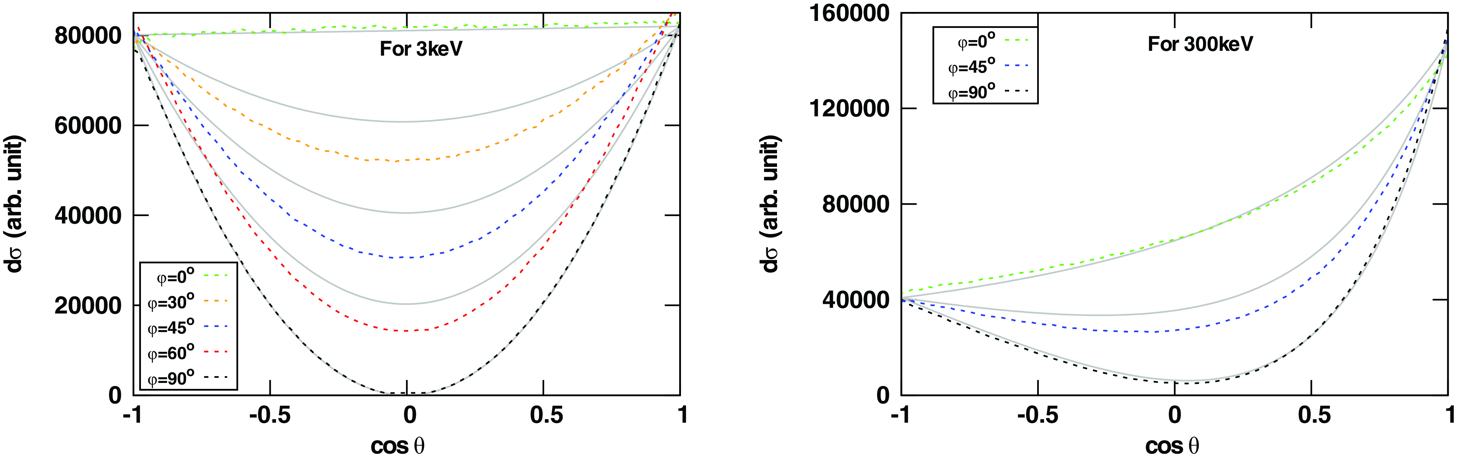
Figure 4. The Klein–Nishina cross section as a function of $\theta$
for a completely polarised incident photon of polarisation angle
$\theta$
for a completely polarised incident photon of polarisation angle $\phi = \theta_e$
. The dashed curves are calculated one by MC method using the equation (1) while the gray solid curves are analytic one expressed by equation (10) and the observed mismatched is due to the approximation involved in equation (10), see the text for details. The left and right panels are for incident photon energy 3 and 300 keV, respectively, and the dashed green, orange, blue, red, and black curves are for
$\phi = \theta_e$
. The dashed curves are calculated one by MC method using the equation (1) while the gray solid curves are analytic one expressed by equation (10) and the observed mismatched is due to the approximation involved in equation (10), see the text for details. The left and right panels are for incident photon energy 3 and 300 keV, respectively, and the dashed green, orange, blue, red, and black curves are for $\theta_e$
= 0, 30, 45, 60, and 90 degree, respectively.
$\theta_e$
= 0, 30, 45, 60, and 90 degree, respectively.
In Fig. 5, we show the PD as a function of $\theta$
for single scattered completely polarised photons of energy 3 keV. We find that the MC results agree with the corresponding theoretical PD (shown by gray solid curve) expressed by equation (12). Here we remind that the positive value of PD signifies that the scattered photons polarisation is perpendicular to the scattering plane while the polarisation is along the scattering plane for negative value. In Fig. 6, we show the modulation curves of single scattered polarised photons for a fixed
$\theta$
for single scattered completely polarised photons of energy 3 keV. We find that the MC results agree with the corresponding theoretical PD (shown by gray solid curve) expressed by equation (12). Here we remind that the positive value of PD signifies that the scattered photons polarisation is perpendicular to the scattering plane while the polarisation is along the scattering plane for negative value. In Fig. 6, we show the modulation curves of single scattered polarised photons for a fixed $\theta$
. We have computed the results for four different polarisation angles of incident photons of energy 3 keV. For
$\theta$
. We have computed the results for four different polarisation angles of incident photons of energy 3 keV. For $\phi$
= 0, the equation (14) predicts that the modulation curve is independent of
$\phi$
= 0, the equation (14) predicts that the modulation curve is independent of $\theta$
in Thomson regime, we find same here see the top left panel. In general, these modulation curves will be described by the equation (14).
$\theta$
in Thomson regime, we find same here see the top left panel. In general, these modulation curves will be described by the equation (14).
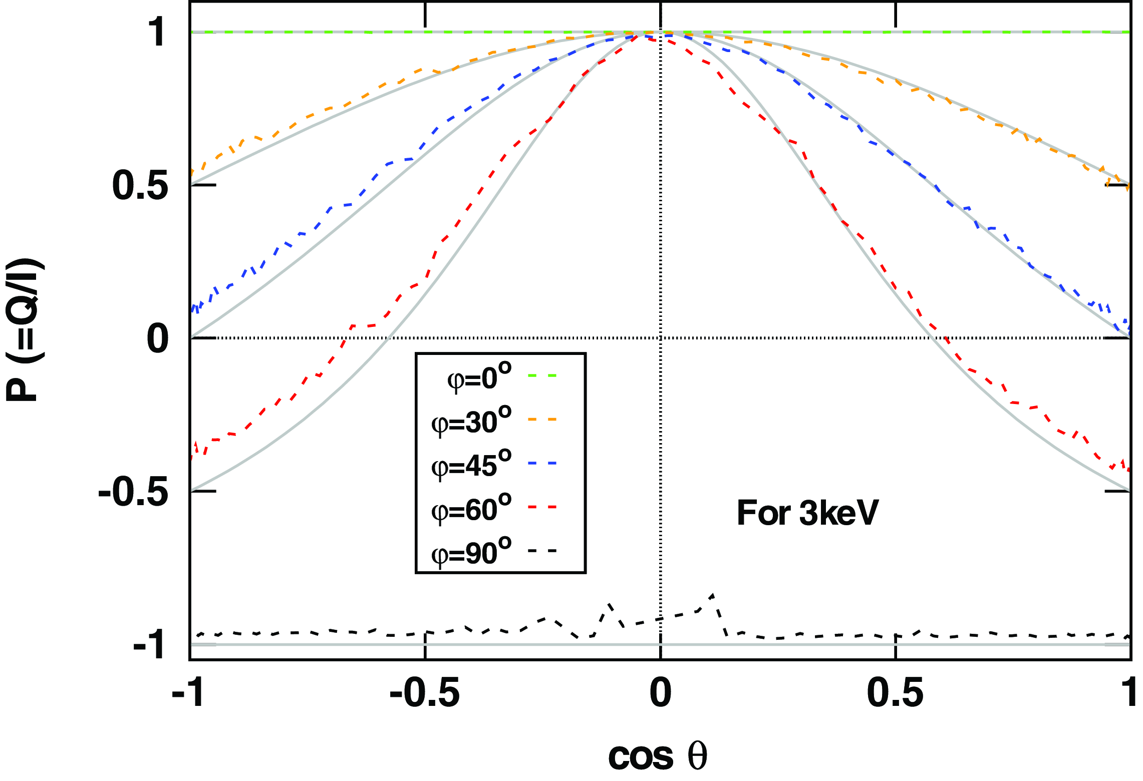
Figure 5. The degree of polarisation after single scattering of completely polarised (incident) photons of energy 3 keV as a function of scattering angle for five different polarisation angle. Here, the dashed green, orange, blue, red, and black curves are for $\theta_e$
= 0, 30, 45, 60, and 90 degree, respectively, and the solid gray curves are an analytical one expressed by equation (12).
$\theta_e$
= 0, 30, 45, 60, and 90 degree, respectively, and the solid gray curves are an analytical one expressed by equation (12).

Figure 6. The modulation curves after single scattering of completely polarised (incident) photons of energy 3 keV for a given $\theta$
. The solid blue, orange, green, red, and cyan curves are for
$\theta$
. The solid blue, orange, green, red, and cyan curves are for $\theta$
= 0, 30, 45, 60, and 90 degree, respectively. The first (top), 2nd, 3rd, and 4th (last) panels are for
$\theta$
= 0, 30, 45, 60, and 90 degree, respectively. The first (top), 2nd, 3rd, and 4th (last) panels are for $\theta_e$
= 0, 30, 45, and 90 degree, respectively. The curves are described analytically by equation (14).
$\theta_e$
= 0, 30, 45, and 90 degree, respectively. The curves are described analytically by equation (14).
5. Modulation curve in perpendicular plane of incident photon for
$\theta <$
25
$^{\circ}$
: A detector working principle


In this section, we examine the result of Section 2.3, and are interested to find the range of $\theta$
in which the polarisation properties of incident photons can be derived from the modulation curve of scattered photons. Motivation for this exercise is that the cross section is maximum for
$\theta$
in which the polarisation properties of incident photons can be derived from the modulation curve of scattered photons. Motivation for this exercise is that the cross section is maximum for $\theta = 0$
for polarised/unpolarised photons of any energy (see Figs. 3, 4, respectively). Thus, it is expected practically that on average upto some range of
$\theta = 0$
for polarised/unpolarised photons of any energy (see Figs. 3, 4, respectively). Thus, it is expected practically that on average upto some range of $\theta$
(
$\theta$
( $> 0$
), the polarisation properties of scattered photons at
$> 0$
), the polarisation properties of scattered photons at $\theta = 0$
will dominant over that range of scattered photons. We find that for
$\theta = 0$
will dominant over that range of scattered photons. We find that for $\theta < 25^{\circ}$
(or
$\theta < 25^{\circ}$
(or $\theta \equiv [0,25^{\circ}]$
) one can adequately predict the polarisation properties of k with using the modulation curve for the k
′.
$\theta \equiv [0,25^{\circ}]$
) one can adequately predict the polarisation properties of k with using the modulation curve for the k
′.
In view of practice, we also examine the same by constructing the distribution of projection of $k^{\prime}_{e}$
on the perpendicular plane to k. For this we fix the direction of the incident photon, say k lies along the z-axis. For a polarised photon, the direction of the electric vector is fixed in space, so (
$k^{\prime}_{e}$
on the perpendicular plane to k. For this we fix the direction of the incident photon, say k lies along the z-axis. For a polarised photon, the direction of the electric vector is fixed in space, so ( $k \times k^{\prime}$
) is also fixed. Without loss of generality, we consider (
$k \times k^{\prime}$
) is also fixed. Without loss of generality, we consider ( $k \times k^{\prime}$
) along the x-axis, that is the scattering plane is a (z,y)-plane. It is shown in Fig. 7. Clearly for
$k \times k^{\prime}$
) along the x-axis, that is the scattering plane is a (z,y)-plane. It is shown in Fig. 7. Clearly for $\theta = 0$
, the
$\theta = 0$
, the $k^{\prime}_{e}$
will lie on the (x,y)-plane. For
$k^{\prime}_{e}$
will lie on the (x,y)-plane. For $\theta > 0$
, the
$\theta > 0$
, the $k^{\prime}_{e}$
will not always lie on (x,y)-plane. And, we measure the direction of projection
$k^{\prime}_{e}$
will not always lie on (x,y)-plane. And, we measure the direction of projection $k^{\prime}_{e}$
on (x,y)-plane or the
$k^{\prime}_{e}$
on (x,y)-plane or the $\phi$
-angle of
$\phi$
-angle of $k^{\prime}_{e}$
. The distributions of
$k^{\prime}_{e}$
. The distributions of $\phi$
-angle of
$\phi$
-angle of $k^{\prime}_{e}$
for 3 and 300 keV completely polarised incident photons have been shown in upper panel of Fig. 8 for polarisation angle
$k^{\prime}_{e}$
for 3 and 300 keV completely polarised incident photons have been shown in upper panel of Fig. 8 for polarisation angle $\phi$
= 45
$\phi$
= 45 $^{\circ}$
for five different ranges of
$^{\circ}$
for five different ranges of $\theta$
= [0,7.5
$\theta$
= [0,7.5 $^{\circ}$
], [0,15
$^{\circ}$
], [0,15 $^{\circ}$
], [0,22.5
$^{\circ}$
], [0,22.5 $^{\circ}$
], [0,30
$^{\circ}$
], [0,30 $^{\circ}$
], [0.45
$^{\circ}$
], [0.45 $^{\circ}$
]. We also map the distribution of the
$^{\circ}$
]. We also map the distribution of the $\phi$
-angle of
$\phi$
-angle of $k^{\prime}_{e}$
for three different polarisation angles
$k^{\prime}_{e}$
for three different polarisation angles $\phi$
= 30
$\phi$
= 30 $^{\circ}$
, 45
$^{\circ}$
, 45 $^{\circ}$
, and 60
$^{\circ}$
, and 60 $^{\circ}$
for a fixed
$^{\circ}$
for a fixed $\theta$
range [0,15
$\theta$
range [0,15 $^{\circ}$
], which is shown in the lower panel of Fig. 8. We find that for
$^{\circ}$
], which is shown in the lower panel of Fig. 8. We find that for $\theta$
range
$\theta$
range $\approx [0,25^{\circ}]$
the distribution of projection of
$\approx [0,25^{\circ}]$
the distribution of projection of $k^{\prime}_{e}$
on the perpendicular plane to k after single scattering can estimate the polarisation properties of incident photons k adequately.
$k^{\prime}_{e}$
on the perpendicular plane to k after single scattering can estimate the polarisation properties of incident photons k adequately.
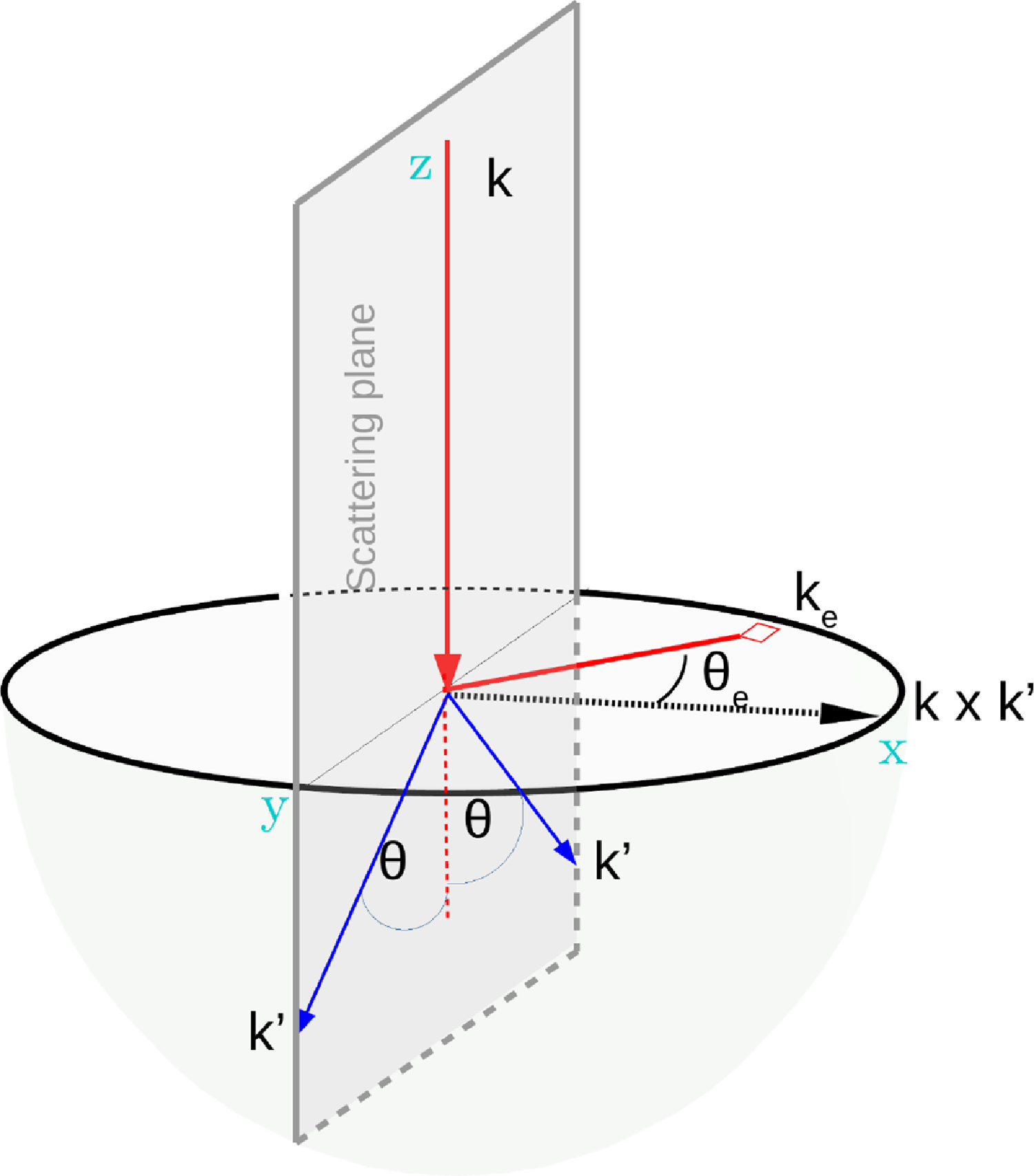
Figure 7. A schematic diagram for calculating the modulation curve in perpendicular plane of incident photon. Here, k is along the z-axis, $(k \times k^{\prime})$
is along the x-axis; thus, the (z,y)-plane is a scattering plane.
$(k \times k^{\prime})$
is along the x-axis; thus, the (z,y)-plane is a scattering plane. $k_e$
with fixed
$k_e$
with fixed $\theta_e$
and k
′ for scattering angle
$\theta_e$
and k
′ for scattering angle $\theta$
are shown.
$\theta$
are shown.

Figure 8. $\phi$
-angle distribution of
$\phi$
-angle distribution of $k^{\prime}_{e}$
after single scattering when the completely polarised photons incident along the z-axis. The upper panel is for the polarisation angle
$k^{\prime}_{e}$
after single scattering when the completely polarised photons incident along the z-axis. The upper panel is for the polarisation angle $\theta_e$
= 45
$\theta_e$
= 45 $^{\circ}$
, and the curves 1, 2, 3, 4 and 5 are for the different ranges of
$^{\circ}$
, and the curves 1, 2, 3, 4 and 5 are for the different ranges of $\theta$ $\equiv$
[0,7.5
$\equiv$
[0,7.5 $^{\circ}$
], [0,15
$^{\circ}$
], [0,15 $^{\circ}$
], [0,22.5
$^{\circ}$
], [0,22.5 $^{\circ}$
], [0,30
$^{\circ}$
], [0,30 $^{\circ}$
], and [0,45
$^{\circ}$
], and [0,45 $^{\circ}$
], respectively. The lower panel is for three different
$^{\circ}$
], respectively. The lower panel is for three different $\theta_e$
at a given range of
$\theta_e$
at a given range of $\theta$ $\equiv$
[0,15
$\equiv$
[0,15 $^{\circ}$
], where the solid red, blue and cyan curves are for
$^{\circ}$
], where the solid red, blue and cyan curves are for $\theta_e$
= 30, 45 and 60
$\theta_e$
= 30, 45 and 60 $^{\circ}$
, respectively, and the orange curves are for unpolarised incident photons. In both panels, the solid and dashed curves are for incident photon energy 3 and 300 keV, respectively, and the dotted curve is simply
$^{\circ}$
, respectively, and the orange curves are for unpolarised incident photons. In both panels, the solid and dashed curves are for incident photon energy 3 and 300 keV, respectively, and the dotted curve is simply $a(\cos\!(2(\phi-\theta_e))+1)$
, a is the normalisation factor.
$a(\cos\!(2(\phi-\theta_e))+1)$
, a is the normalisation factor.
As understood, the detector has to estimate the polarisation properties of the observed photons. And, for Compton/ Thomson scattering based detector (like, AstroSat/CZTI, PoGo+, POLAR, POLIX, etc Fabiani Reference Fabiani2018) the observed photons are essentially an incident photon, and so the above analysis is more relevant for a detector as a working principle. However, the above discussed are only the essential criteria for the detector designing and for the general mechanism for a specific detector please see the relevant references, like (Lei et al. Reference Lei, Dean and Hills1997; Fabiani Reference Fabiani2018; Chattopadhyay et al. Reference Chattopadhyay, Vadawale, Rao, Sreekumar and Bhattacharya2014, and references therein).
6. Polarisation measurement along a meridian plane after single scattering
We aim to estimate the degree of polarisation and angle of polarisation for the emergent photons from a given meridian plane after single scattering where unpolarised incident photons lie on any appropriate plane. For this we consider a simplistic (without loss of generality) geometry a semi-spherical shell where the incident photon generates at center of the shell and we specify its direction in spherical coordinate by ( $\theta_i, \phi_i$
), that is, on meridian
$\theta_i, \phi_i$
), that is, on meridian $\phi_i$
-plane. We are interested to compute the P and
$\phi_i$
-plane. We are interested to compute the P and $\chi$
for the scattered photon (
$\chi$
for the scattered photon ( $\theta_s, \phi_s$
), or in general, to compute the
$\theta_s, \phi_s$
), or in general, to compute the $P\ \&\ \chi$
as a function of
$P\ \&\ \chi$
as a function of $\theta_s$
on the meridian
$\theta_s$
on the meridian $\phi_s$
-plane.
$\phi_s$
-plane.
Before discussing the general results, we first discuss, for clarity, a few simplistic cases in terms of incident photon direction (k), or scattering plane (or $(k \times k^{\prime})$
), or combination of both in the following sections. To measure the angle of polarisation one needs a reference direction of (
$(k \times k^{\prime})$
), or combination of both in the following sections. To measure the angle of polarisation one needs a reference direction of ( $k \times k^{\prime}$
) for the next scattering, we consider that (
$k \times k^{\prime}$
) for the next scattering, we consider that ( $k \times k^{\prime}$
)-next lies on the same scattered meridian plane, and we take its direction as (
$k \times k^{\prime}$
)-next lies on the same scattered meridian plane, and we take its direction as ( $\theta_s+\pi/2,\phi_s$
). However, we will first discuss the way of computing the averaged PD and PA of the scattered photons, as we are caring now the orientation of the scattering plane.
$\theta_s+\pi/2,\phi_s$
). However, we will first discuss the way of computing the averaged PD and PA of the scattered photons, as we are caring now the orientation of the scattering plane.
6.1. Averaged degree of polarisation
The partially polarised incident photons of degree of polarisation $p_I$
and the angle of polarisation
$p_I$
and the angle of polarisation $\phi_I$
can be an average behaviour of total n type of incident photons which have different degree and angle of polarisation, say
$\phi_I$
can be an average behaviour of total n type of incident photons which have different degree and angle of polarisation, say $p_j$
and
$p_j$
and $\phi_j$
for
$\phi_j$
for $j^{th}$
type incident photons, respectively. In context of Compton scattering, it can be expressed for
$j^{th}$
type incident photons, respectively. In context of Compton scattering, it can be expressed for $\xi$
-angle variable as (using equation (16)):
$\xi$
-angle variable as (using equation (16)):
 \begin{equation} p_I \cos\!(2(\xi+\phi_I)) + 1 = \sum_{J=1}^n \frac{1}{n}[p_j \cos\!(2(\xi+\phi_j)) + 1 ],\end{equation}
For example, one has unpolarised photons which is a combination of two types of photon with $p_1 =p_0, \phi_1 =\phi_0$
and
$p_1 =p_0, \phi_1 =\phi_0$
and $p_2 = p_0$
,
$p_2 = p_0$
, $\phi_2=\phi_o+\pi/2$
. It would be true for any value of
$\phi_2=\phi_o+\pi/2$
. It would be true for any value of $p_0$
(e.g.
$p_0$
(e.g. $p_0 = 1$
). We use this characteristic to estimate the PD and PA for emergent photons either after single scattering or multi scattering. For this we compute the
$p_0 = 1$
). We use this characteristic to estimate the PD and PA for emergent photons either after single scattering or multi scattering. For this we compute the $\chi_j$
(PA of the
$\chi_j$
(PA of the $j\mathrm{ th}$
type scattered photons) using equation (11), as
$j\mathrm{ th}$
type scattered photons) using equation (11), as $\tan 2\chi_j = \frac{U}{Q}$
, and compute the averaged
$\tan 2\chi_j = \frac{U}{Q}$
, and compute the averaged $p_j$
(over
$p_j$
(over $\phi$
, PA of the incident photons) as a function of
$\phi$
, PA of the incident photons) as a function of $\theta$
as,
$\theta$
as, $p_j$
=
$p_j$
= $\frac{\langle Q\rangle}{\langle I\rangle}$
.
$\frac{\langle Q\rangle}{\langle I\rangle}$
.
6.2. Case I: Fixed k direction (along z-axis) for a given scattering plane
We first consider a simplistic situation in which the unpolarised photons incident along the z-direction, and we fix the scattering plane to $\phi_s$
-plane, that is, the (
$\phi_s$
-plane, that is, the ( $k\times k^{\prime}$
) direction is (
$k\times k^{\prime}$
) direction is ( $\pi/2, \phi_s+\pi/2$
). Since, the scattering plane is the same as the interested meridian
$\pi/2, \phi_s+\pi/2$
). Since, the scattering plane is the same as the interested meridian $\phi_s$
-plane; thus, the scattering angle is
$\phi_s$
-plane; thus, the scattering angle is $\theta = \theta_s$
. And so P will follow equation (7) with
$\theta = \theta_s$
. And so P will follow equation (7) with $\theta = \theta_s$
. The
$\theta = \theta_s$
. The $\chi$
is always 90 degree (with the choice of (
$\chi$
is always 90 degree (with the choice of ( $k\times k^{\prime}$
)-next), it means that the
$k\times k^{\prime}$
)-next), it means that the $k^{\prime}_{e}$
lies parallel to the (x, y)-plane. The result (for
$k^{\prime}_{e}$
lies parallel to the (x, y)-plane. The result (for $\theta_i$
=0) is shown in the 2nd column of Table 1. In addition, similarly, for a fully polarised incident photons the PD will be determined by equation (12).
$\theta_i$
=0) is shown in the 2nd column of Table 1. In addition, similarly, for a fully polarised incident photons the PD will be determined by equation (12).
Table 1. The PD (P) and PA ( $\chi$
) of the emergent photons as a function of
$\chi$
) of the emergent photons as a function of $\theta_s$
(or i) for cases I and II. The results for case II are presented for six different scattered meridian planes
$\theta_s$
(or i) for cases I and II. The results for case II are presented for six different scattered meridian planes $\phi_i + \phi_{is}$
with
$\phi_i + \phi_{is}$
with $\phi_{is}$
= 15, 30, 45, 60, 75, and 90 degree. While the results for case I are true for any scattered meridian plane, as here
$\phi_{is}$
= 15, 30, 45, 60, 75, and 90 degree. While the results for case I are true for any scattered meridian plane, as here $\phi_s$
-plane =
$\phi_s$
-plane = $\phi_i$
-plane, and computed for two different ranges of
$\phi_i$
-plane, and computed for two different ranges of $\theta_i$
= 0 and [0,
$\theta_i$
= 0 and [0, $\pi$
].
$\pi$
].

1: here $\phi_{si}$
is measured in anti-clockwise direction, if it is measured in clockwise direction then the angle of polarisation becomes
$\phi_{si}$
is measured in anti-clockwise direction, if it is measured in clockwise direction then the angle of polarisation becomes $\pi-\chi$
.
$\pi-\chi$
.
Instead of taking incident photons along the $z-$
axis (or
$z-$
axis (or $\theta_i=0$
), we also consider any direction of k on incident meridian
$\theta_i=0$
), we also consider any direction of k on incident meridian $\phi_i-$
plane, that is, the range of
$\phi_i-$
plane, that is, the range of $\theta_i$
is
$\theta_i$
is $\theta_i \equiv [0,\pi]$
. And we assume again that the scattering plane is the same as the interested meridian
$\theta_i \equiv [0,\pi]$
. And we assume again that the scattering plane is the same as the interested meridian $\phi_s$
-plane. In this case, we expect a constant P
$\phi_s$
-plane. In this case, we expect a constant P $\sim$
0.33, as shown by the red curve in the right panel of Fig. 3. We find almost the same and show the results in the 3rd column of Table 1.
$\sim$
0.33, as shown by the red curve in the right panel of Fig. 3. We find almost the same and show the results in the 3rd column of Table 1.
6.3. Case II: (
$k \times k^{\prime}$
) lies on the meridian plane of k

In the previous case, the scattering plane and interested meridian plane are the same. Next, we consider that incident photons and the ( $k \times k^{\prime}$
) both lie on the same
$k \times k^{\prime}$
) both lie on the same $\phi_i$
-meridian plane, so (
$\phi_i$
-meridian plane, so ( $k \times k^{\prime}$
)’s direction for a given k is (
$k \times k^{\prime}$
)’s direction for a given k is ( $\theta_i+\pi/2, \phi_i$
). Now the photons will scattered any meridian (
$\theta_i+\pi/2, \phi_i$
). Now the photons will scattered any meridian ( $\phi_i+\phi_{is}$
)-plane, in which
$\phi_i+\phi_{is}$
)-plane, in which $\phi_{is}$
is the angle between incident and scattered meridian plane and the range of
$\phi_{is}$
is the angle between incident and scattered meridian plane and the range of $\phi_{is}$
is
$\phi_{is}$
is $\equiv$
[
$\equiv$
[ $-\pi, \pi$
]. For
$-\pi, \pi$
]. For $\theta_i$
= 0 and
$\theta_i$
= 0 and $\pi/2$
, the scattering plane of k is
$\pi/2$
, the scattering plane of k is $(\phi_i \pm \pi/2)$
-plane and
$(\phi_i \pm \pi/2)$
-plane and $(\theta = \pi/2)$
-plane, respectively. In general, the scattering plane of k will must pass the line (
$(\theta = \pi/2)$
-plane, respectively. In general, the scattering plane of k will must pass the line ( $\pi/2,\phi_i+\pi/2$
) (i.e. rotated y-axis with angle
$\pi/2,\phi_i+\pi/2$
) (i.e. rotated y-axis with angle $\phi_i$
about z-axis, say y
′-axis), or in other words it is a rotation of
$\phi_i$
about z-axis, say y
′-axis), or in other words it is a rotation of $(\phi_i \pm \pi/2)$
-plane about y
′-axis with same angle
$(\phi_i \pm \pi/2)$
-plane about y
′-axis with same angle $\theta_i$
. Thus, except for scattered meridian
$\theta_i$
. Thus, except for scattered meridian $(\phi_i \pm\pi/2)$
-plane, the k
′ arises uniquely on a different scattering plane with different
$(\phi_i \pm\pi/2)$
-plane, the k
′ arises uniquely on a different scattering plane with different $\theta$
. For example, for the meridian
$\theta$
. For example, for the meridian $(\phi_i+\pi/6)$
-plane the
$(\phi_i+\pi/6)$
-plane the $\theta$
varies from
$\theta$
varies from $\pi/6$
to zero, and
$\pi/6$
to zero, and $\chi$
varies from zero to
$\chi$
varies from zero to $\pi/6$
, when
$\pi/6$
, when $\theta_s$
varies from
$\theta_s$
varies from $\pi/2$
to zero. The degree of polarisation will simply determine by using equation (7), and in general, for a given scattered meridian
$\pi/2$
to zero. The degree of polarisation will simply determine by using equation (7), and in general, for a given scattered meridian $(\phi_i+\phi_{is})$
-plane the P varies from
$(\phi_i+\phi_{is})$
-plane the P varies from $P(\theta=\phi_{is})$
of equation (7) to zero for the variation of
$P(\theta=\phi_{is})$
of equation (7) to zero for the variation of $\theta_s$
from
$\theta_s$
from $\pi/2$
to zero, respectively. The results for P as a function of
$\pi/2$
to zero, respectively. The results for P as a function of $\theta_s$
for 6 different meridian planes with
$\theta_s$
for 6 different meridian planes with $\phi_{is}$
= 15, 30, 45, 60, 75, and 90 degree are shown in Table 1.
$\phi_{is}$
= 15, 30, 45, 60, 75, and 90 degree are shown in Table 1.
6.4. Case III: Any fixed incident photon direction and a random scattering plane
Next, we fix the k direction ( $\theta_i,\phi_i$
) and take all possible directions of (
$\theta_i,\phi_i$
) and take all possible directions of ( $k \times k^{\prime}$
) on a perpendicular plane to k. Like case II, the incident photon is scattered in all directions. For a given meridian plane, each k
′ is arisen from a different direction of (
$k \times k^{\prime}$
) on a perpendicular plane to k. Like case II, the incident photon is scattered in all directions. For a given meridian plane, each k
′ is arisen from a different direction of ( $k \times k^{\prime}$
), and clearly the different
$k \times k^{\prime}$
), and clearly the different $\theta$
. The PD can be determined using equation (7) for known
$\theta$
. The PD can be determined using equation (7) for known $\theta$
. Since, the scattering plane is unique for a given k
′, like PD, PA will be also unique. We have computed the P and
$\theta$
. Since, the scattering plane is unique for a given k
′, like PD, PA will be also unique. We have computed the P and $\chi$
for the meridian plane ranges from
$\chi$
for the meridian plane ranges from $\phi_i$
to
$\phi_i$
to $\phi_i +\pi$
, and for each meridian plane
$\phi_i +\pi$
, and for each meridian plane $\theta_i$
ranges from 0 to
$\theta_i$
ranges from 0 to $\pi/2$
. It should be noted that case III is identical to case I for
$\pi/2$
. It should be noted that case III is identical to case I for $\theta_i$
= 0.
$\theta_i$
= 0.
6.5. Case IV: k lies on the surface of cone at centre with opening angle
$\theta_i$
and a random scattering plane

We extend the case III with considering that $\theta_i$
of k is still fix but now
$\theta_i$
of k is still fix but now $\phi_i$
can take any value in [0,2
$\phi_i$
can take any value in [0,2 $\pi$
], so essentially the vector k is rotating on the surface of the cone of opening angle
$\pi$
], so essentially the vector k is rotating on the surface of the cone of opening angle $\theta_i$
which is situated at the centre. Unlike Case II or III, here on a given meridian plane the k
′ is arisen by any k with appropriate scattering angle; thus, PD and PA of k
′ would be estimated by averaging method. The averaged P and
$\theta_i$
which is situated at the centre. Unlike Case II or III, here on a given meridian plane the k
′ is arisen by any k with appropriate scattering angle; thus, PD and PA of k
′ would be estimated by averaging method. The averaged P and $\chi$
of the k
′ are computed using equation (18) for a given
$\chi$
of the k
′ are computed using equation (18) for a given $\theta_s$
, where now, n is total no. of scattered photons with
$\theta_s$
, where now, n is total no. of scattered photons with $\theta_s$
, the
$\theta_s$
, the $p_j$
is determined for each scattered photon for known
$p_j$
is determined for each scattered photon for known $\theta$
by using equation (7). Since, for unpolarised incident photons the
$\theta$
by using equation (7). Since, for unpolarised incident photons the $k^{\prime}_{e}$
lies along the
$k^{\prime}_{e}$
lies along the $(k\times k^{\prime})$
which gives
$(k\times k^{\prime})$
which gives $\phi_j$
= 0, but we have fixed the reference
$\phi_j$
= 0, but we have fixed the reference $(k\times k^{\prime})\text{-next}$
to measure the PA, so
$(k\times k^{\prime})\text{-next}$
to measure the PA, so $\phi_j$
is the angle between
$\phi_j$
is the angle between $(k\times k^{\prime})$
and meridian plane (
$(k\times k^{\prime})$
and meridian plane ( $(k\times k^{\prime})$
-next). Expectedly, the variation of P, and
$(k\times k^{\prime})$
-next). Expectedly, the variation of P, and $\chi$
as a function of
$\chi$
as a function of $\theta_s$
is same for all scattered meridian planes. In Table 2, we have noted the results for
$\theta_s$
is same for all scattered meridian planes. In Table 2, we have noted the results for $\theta_i$
= 0, 15, 30, 45, 60, 75, and 90 degree along with
$\theta_i$
= 0, 15, 30, 45, 60, 75, and 90 degree along with $f_{\theta_s}$
(a total no. of scattered emergent photons with
$f_{\theta_s}$
(a total no. of scattered emergent photons with $\theta_s$
on a given meridian plane). For example, the emergent photons along the z-axis (
$\theta_s$
on a given meridian plane). For example, the emergent photons along the z-axis ( $\theta_s$
=0) are unpolarised for any opening angle
$\theta_s$
=0) are unpolarised for any opening angle $\theta_i$
, as in this case for all incident photons the scattering angle is
$\theta_i$
, as in this case for all incident photons the scattering angle is $\theta = \theta_i$
, and the electric vector of k
′ is isotropically distributed. In general, for a given
$\theta = \theta_i$
, and the electric vector of k
′ is isotropically distributed. In general, for a given $\theta_i$
, the emergent photons escape maximally at
$\theta_i$
, the emergent photons escape maximally at $\theta_s$ $\sim$ $\theta_i$
, for example, for
$\theta_i$
, for example, for $\theta_i$
= 15
$\theta_i$
= 15 $^{\circ}$
the maximum emergent photons escape with
$^{\circ}$
the maximum emergent photons escape with $\theta_s$ $\sim$
25
$\sim$
25 $^{\circ}$
and have PD
$^{\circ}$
and have PD $\sim$
0.06.
$\sim$
0.06.
Table 2. The PD and PA of the emergent photons for case IV along with $f_{\theta_s}$
(total no. of the emergent photons for a given
$f_{\theta_s}$
(total no. of the emergent photons for a given $\theta_s$
). The results are presented for seven different opening angles of cone (on which incident photon lies),
$\theta_s$
). The results are presented for seven different opening angles of cone (on which incident photon lies), $\theta_i$
= 0, 15, 30, 45, 60, 75, and 90 degree.
$\theta_i$
= 0, 15, 30, 45, 60, 75, and 90 degree.

*the corresponding value is not reliable due to low statistics.
Note: for $\theta_i = \theta_s$
, one has small P (in range of (0.002-0.08)) and maximum
$\theta_i = \theta_s$
, one has small P (in range of (0.002-0.08)) and maximum $f_{\theta_s}$
.
$f_{\theta_s}$
.
We compare the above results with the results of case III. Since the given k
′ can be arisen from the incident meridian ( $\phi_s+\phi_{is}$
)-plane with
$\phi_s+\phi_{is}$
)-plane with $\phi_{is}$ $\equiv$
[−
$\equiv$
[− $\pi$
,
$\pi$
, $\pi$
] of case III, or particularly n different situations of case III in range of
$\pi$
] of case III, or particularly n different situations of case III in range of $\phi_i$ $\equiv$ $[0,2\pi]$
. As the P and
$[0,2\pi]$
. As the P and $\chi$
of case III are uniquely determined for a given
$\chi$
of case III are uniquely determined for a given $\phi_{is}$
, the resultant P and
$\phi_{is}$
, the resultant P and $\chi$
of case IV for a given
$\chi$
of case IV for a given $\theta_s$
can be obtained by weighted averaging method, as defined in equation (18). For present case this equation is rewritten as:
$\theta_s$
can be obtained by weighted averaging method, as defined in equation (18). For present case this equation is rewritten as:
 \begin{equation} P \cos\!(2(\xi+\chi)) + 1 = \sum_{j=1}^{n} f_j \left [p_j\cos\!(2(\xi+\chi_j))+1\right], \end{equation}
here, $f_{j}$
is the fraction of emergent scattered photons at
$f_{j}$
is the fraction of emergent scattered photons at $\theta_s$
to total that arisen due to the
$\theta_s$
to total that arisen due to the $j\mathrm{th}$
incident meridian
$j\mathrm{th}$
incident meridian $(\phi_s+\phi_{is})$
-plane, and
$(\phi_s+\phi_{is})$
-plane, and $p_j$
, and
$p_j$
, and $\chi_j$
are corresponding PD and PA, respectively. We find that the results are similar in both ways.
$\chi_j$
are corresponding PD and PA, respectively. We find that the results are similar in both ways.
6.6. Case V: General case
Finally, we consider a general case where there is no restriction on k. That is, the scattered photon k
′ is arising from all directions of k. We compute the P as a function of $\theta_s$
for any meridian
$\theta_s$
for any meridian $\phi_s$
-plane, We find P
$\phi_s$
-plane, We find P $\approx$
11, 0
$\approx$
11, 0 $\%$
for
$\%$
for $\theta_s$
= 90, 0 degree, respectively. The
$\theta_s$
= 90, 0 degree, respectively. The $\chi$
is
$\chi$
is $\sim$
90 degree for all
$\sim$
90 degree for all $\theta_s$
. Since we are measuring
$\theta_s$
. Since we are measuring $\chi$
with respect to
$\chi$
with respect to $(k\times k^{\prime})$
-next, it signifies that
$(k\times k^{\prime})$
-next, it signifies that $k^{\prime}_{e}$
is parallel to the (x,y)-plane. Clearly, the all scattering planes (which generate the k
′ on
$k^{\prime}_{e}$
is parallel to the (x,y)-plane. Clearly, the all scattering planes (which generate the k
′ on $\phi_s$
-plane) are not a
$\phi_s$
-plane) are not a $\phi_s$
-plane, but we notice that on averaged the scattering plane is mostly a scattered meridian plane; thus, the results
$\phi_s$
-plane, but we notice that on averaged the scattering plane is mostly a scattered meridian plane; thus, the results $\chi$ $\sim$
90
$\sim$
90 $^{\circ}$
confirm that the polarisation of single scattered unpolarised (incident) photons is perpendicular to the scattering plane. The results are shown in Table 3.
$^{\circ}$
confirm that the polarisation of single scattered unpolarised (incident) photons is perpendicular to the scattering plane. The results are shown in Table 3.
Table 3. The PD of the emergent photons for general case V from any given meridian plane after single scattering of the randomly oriented unpolarised incident photons (or, the re-estimation of laws of darkening of Chandrasekhar (Reference Chandrasekhar1946) with having a general Klein–Nishina cross section, equation (1)).
Like case IV, the results of case V are verified by a weighted averaging method using the result of case IV. For convenience in Table 2 we have also listed the $f_{\theta_s}$
along with the P and
$f_{\theta_s}$
along with the P and $\chi$
. Thus,
$\chi$
. Thus, $f_j = \frac{f_{\theta_s}}{\Sigma_{j=1}^n f_{\theta_s}}$
for a given
$f_j = \frac{f_{\theta_s}}{\Sigma_{j=1}^n f_{\theta_s}}$
for a given $\theta_s$
and
$\theta_s$
and $\theta_i$
(here,
$\theta_i$
(here, $i=j$
), and with having
$i=j$
), and with having $n = 7$
we obtain the results of case V approximately using Table 2 and equation (19).
$n = 7$
we obtain the results of case V approximately using Table 2 and equation (19).
The results are qualitatively agreed with almost century old calculations of Chandrasekhar (Reference Chandrasekhar1946) (see also, Chandrasekhar Reference Chandrasekhar1960). Chandrasekhar (Reference Chandrasekhar1946) had solved the radiative transfer equations, which is governed by the Thomson scattering by free electron, for the intensities of two states of polarisation, one $I_l$
is along the meridian plane and other one
$I_l$
is along the meridian plane and other one $I_r$
is perpendicular to it, with no incident radiation. In defining the source function for
$I_r$
is perpendicular to it, with no incident radiation. In defining the source function for $I_l$
or
$I_l$
or $I_r$
, the considered cross section for the polarisation in perpendicular to and parallel to the scattering plane is either for unpolarised photons, or combinations of two polarised photons with polarisation angle
$I_r$
, the considered cross section for the polarisation in perpendicular to and parallel to the scattering plane is either for unpolarised photons, or combinations of two polarised photons with polarisation angle $\phi$
and
$\phi$
and $\phi + \pi/2$
, see equations (2) and (3) of their paper and table 2 for the results (and for refined results see table XXIV in Chandrasekhar Reference Chandrasekhar1960). So, the laws of darkening for the PD of the emergent photon is only for the single scattering event in Thomson regime for unpolarised incident photons. In the next section, we compute the laws of darkening for multi scattering events.
$\phi + \pi/2$
, see equations (2) and (3) of their paper and table 2 for the results (and for refined results see table XXIV in Chandrasekhar Reference Chandrasekhar1960). So, the laws of darkening for the PD of the emergent photon is only for the single scattering event in Thomson regime for unpolarised incident photons. In the next section, we compute the laws of darkening for multi scattering events.
For all cases, we have estimated the PD and PA by two another methods, (i) we perform second scattering and construct the modulation curve for either $\theta = 0$
or
$\theta = 0$
or $\theta \equiv [0,25^{\circ}]$
to estimate the P as discussed in Section 2.3, (ii) we construct the modulation curve using the probability
$\theta \equiv [0,25^{\circ}]$
to estimate the P as discussed in Section 2.3, (ii) we construct the modulation curve using the probability $p(\eta)$
(of equation (17)) and estimate the P, as discussed in Section 4.1. We find that in all cases the results match qualitatively with these two methods.
$p(\eta)$
(of equation (17)) and estimate the P, as discussed in Section 4.1. We find that in all cases the results match qualitatively with these two methods.
7. General results and comparison with observations
In the previous section, we estimate the polarisation for a single scattering event in Thomson regime and for a almost rest electron. In this section we consider a multi scattering event with arbitrary electron Lorentz factor. We explore the general results for spectro-polarimatric measurement for XRBs source and make a comparision for few XRBs observed by IXPE. In general, a detailed accretion disc + corona geometry is required for the spectro-polarimatric study for XRBs (e.g. Beheshtipour et al. Reference Beheshtipour, Krawczynski and Malzac2017; Schnittman & Krolik Reference Schnittman and Krolik2010). However, here to estimate the polarisation for multi scattering events and the energy dependency of polarisation, for completeness we consider the same spherical corona geometry (as described in Section 3). Therefore, our results will describe the observed polarisation properties qualitatively only.
7.1. Multi-scattering
To verify the MC calculations for multi scattering we consider the case I with $\theta_i \equiv [0,\pi]$
, as in this case the scattered photon has PD
$\theta_i \equiv [0,\pi]$
, as in this case the scattered photon has PD $\sim$
0.33 in all directions of
$\sim$
0.33 in all directions of $\theta_s$
. We first compute (say, first method) the P value of 2nd times scattered photon for this case. Next, we consider (say, 2nd method) a partially polarised incident photon with P = 0.33,
$\theta_s$
. We first compute (say, first method) the P value of 2nd times scattered photon for this case. Next, we consider (say, 2nd method) a partially polarised incident photon with P = 0.33, $\chi$
= 90 degree and
$\chi$
= 90 degree and $(k \times k^{\prime})$
lies either on the meridian plane or perpendicular to the meridian plane (and here, for 0.66 fraction of unpolarised photons, the
$(k \times k^{\prime})$
lies either on the meridian plane or perpendicular to the meridian plane (and here, for 0.66 fraction of unpolarised photons, the $(k \times k^{\prime})$
lies randomly) and estimate the P after single scattering. We find that for both methods the result qualitatively agrees, with P
$(k \times k^{\prime})$
lies randomly) and estimate the P after single scattering. We find that for both methods the result qualitatively agrees, with P $\sim 0.1-0.12$
on a given meridian plane.
$\sim 0.1-0.12$
on a given meridian plane.
Interestingly, we find that for all cases, I $-$
V, after 3-4 numbers of scattering, the maximum P value is reduced to
$-$
V, after 3-4 numbers of scattering, the maximum P value is reduced to $\sim$ $0.02 - 0.05$
on any meridian plane. Here, again we consider a Thomson regime and almost rest electron. Therefore, for all cases and average scattering number
$0.02 - 0.05$
on any meridian plane. Here, again we consider a Thomson regime and almost rest electron. Therefore, for all cases and average scattering number $>$
4, the emergent scattered photon is mainly unpolarised with averaged maximum
$>$
4, the emergent scattered photon is mainly unpolarised with averaged maximum $P \sim 0.035$
. Here, we like to point out that if these emergent photons again freshly scatter in optically thin corona with average scattering number
$P \sim 0.035$
. Here, we like to point out that if these emergent photons again freshly scatter in optically thin corona with average scattering number $\sim$
1 then the P
$\sim$
1 then the P $\&$
$\&$ $\chi$
will be described like case V.
$\chi$
will be described like case V.
7.2. Energy dependency of polarisation
The prime focus is here to study the polarisation properties for XRBs, and XRBs frequently transit from soft spectral state to hard state and vice versa. To understand and to explore the energy dependency of polarisation for Comptonised photons, we consider two different steady spectral states with unpolarised seed photons. The first is a soft spectrum (Model 1) with low electron medium temperature $kT_e$ $= 2.5$
keV (see, e.g. Kumar & Misra Reference Kumar and Misra2014). In view of neutron star NS low-mass XRBs, we consider two different seed photon source (black body) temperatures corresponding to Hot-seed and Cold-seed photon model (see, e.g. Kumar & Misra Reference Kumar and Misra2016a, references therein) which are
$= 2.5$
keV (see, e.g. Kumar & Misra Reference Kumar and Misra2014). In view of neutron star NS low-mass XRBs, we consider two different seed photon source (black body) temperatures corresponding to Hot-seed and Cold-seed photon model (see, e.g. Kumar & Misra Reference Kumar and Misra2016a, references therein) which are $kT_b$ $=$
1.5 and 0.7 keV, respectively. We refer Model 1a with temperature
$=$
1.5 and 0.7 keV, respectively. We refer Model 1a with temperature $kT_e =$
2.5 keV and
$kT_e =$
2.5 keV and $kT_b =$
1.5 keV and for Model 1b
$kT_b =$
1.5 keV and for Model 1b $kT_e =$
2.5 keV and
$kT_e =$
2.5 keV and $kT_b =$
0.7 keV. Since, for consistency we consider only a spherical corona geometry, but these two models are defined based on the seed photon source geometry (e.g. Lin et al. Reference Lin, Remillard and Homan2007); thus, our study does not give physical insight of the model but only provides the dependency of PD and PA on
$kT_b =$
0.7 keV. Since, for consistency we consider only a spherical corona geometry, but these two models are defined based on the seed photon source geometry (e.g. Lin et al. Reference Lin, Remillard and Homan2007); thus, our study does not give physical insight of the model but only provides the dependency of PD and PA on $kT_b$
variations. The second is a hard spectrum (Model 2) with high electron medium temperature
$kT_b$
variations. The second is a hard spectrum (Model 2) with high electron medium temperature $kT_e =$
100 keV and
$kT_e =$
100 keV and $kT_b =$
0.3 keV. To explore the general results we take two optical depth values in such a way that the corresponding average scattering number
$kT_b =$
0.3 keV. To explore the general results we take two optical depth values in such a way that the corresponding average scattering number $\langle N_{sc}\rangle$ $\approx$
1.1 and 5.0. Thus, conclusively to explore the energy dependency of PD and PA, we take mainly three Models 1a, 1b, and 2 with two values of
$\approx$
1.1 and 5.0. Thus, conclusively to explore the energy dependency of PD and PA, we take mainly three Models 1a, 1b, and 2 with two values of $\langle N_{sc}\rangle$ $\approx$
1.1 and 5.0. PD and PA have been computed for four values of
$\approx$
1.1 and 5.0. PD and PA have been computed for four values of $\theta_s$
= 30
$\theta_s$
= 30 $^{\circ}$
, 45
$^{\circ}$
, 45 $^{\circ}$
, 60
$^{\circ}$
, 60 $^{\circ}$
, 75
$^{\circ}$
, 75 $^{\circ}$
. In considered spherical geometry, if one assumes, the z-axis is along the radio-jet direction, then the (x,y)-plane will mimic the accretion disc and so the angle
$^{\circ}$
. In considered spherical geometry, if one assumes, the z-axis is along the radio-jet direction, then the (x,y)-plane will mimic the accretion disc and so the angle $\theta_s$
is equivalent to the disc inclination angle i (or the angle between the line of sight and the normal to the disc plane). Thus, we also study the variation of PD and PA with disc inclination angle i. And now, in present convention, PA = 90
$\theta_s$
is equivalent to the disc inclination angle i (or the angle between the line of sight and the normal to the disc plane). Thus, we also study the variation of PD and PA with disc inclination angle i. And now, in present convention, PA = 90 $^{\circ}$
signifies that the electric vector is parallel to the disc plane.
$^{\circ}$
signifies that the electric vector is parallel to the disc plane.
The general results for Model 1a and 1b are shown in Fig. 9. The upper and lower panels are for $\langle N_{sc}\rangle$ $\approx$
1.1 and 5, respectively. In the left panel, the seed photon flux is shown by dashed curve and Comptonized photon flux by solid line. As expected for
$\approx$
1.1 and 5, respectively. In the left panel, the seed photon flux is shown by dashed curve and Comptonized photon flux by solid line. As expected for $\langle N_{sc}\rangle$ $\approx$
1.1 the PD as a function of
$\approx$
1.1 the PD as a function of $\theta_s$
(or, i) is slightly lower than the respective values listed in Table 3. The PD values for given i are almost constant over the energy bin, also qualitatively independent from the seed photon source temperature
$\theta_s$
(or, i) is slightly lower than the respective values listed in Table 3. The PD values for given i are almost constant over the energy bin, also qualitatively independent from the seed photon source temperature $kT_b$
. Due to the low photons statistics, the PD and PA are computed upto photon energy 8 and 16 keV for Model 1a and 1b, respectively, and we also notice that their values are fluctuated around this energy bin. Since for unpolarised incident photons and for single scattering, it is expected that the electric vector of Comptonized photons will lie normal to the scattering plane. And for
$kT_b$
. Due to the low photons statistics, the PD and PA are computed upto photon energy 8 and 16 keV for Model 1a and 1b, respectively, and we also notice that their values are fluctuated around this energy bin. Since for unpolarised incident photons and for single scattering, it is expected that the electric vector of Comptonized photons will lie normal to the scattering plane. And for $\langle N_{sc}\rangle$ $\approx$
1.1 we find almost the same, here for all i values, the PA lies from 89
$\approx$
1.1 we find almost the same, here for all i values, the PA lies from 89 $^{\circ}$
to 95
$^{\circ}$
to 95 $^{\circ}$
.
$^{\circ}$
.

Figure 9. Comptonized photons density distribution, degree of polarisation and angle of polarisation are shown in left, middle, and right panels, respectively, when the seed photons (shown by dashed line in left panel) are unpolarised. The upper and lower panels are for the average scattering number $\approx$
1.1 and 5, respectively. PD and PA are computed for four
$\approx$
1.1 and 5, respectively. PD and PA are computed for four $\theta_s$
(or, alternatively the disc inclination angle i) values = 30, 45, 60, and 75 degree, which are shown by dashed-dotted, solid, dotted, and dashed lines, respectively. PA is computed on perpendicular plane to the escaped photon directions, not on the sky plane, here PA = 90
$\theta_s$
(or, alternatively the disc inclination angle i) values = 30, 45, 60, and 75 degree, which are shown by dashed-dotted, solid, dotted, and dashed lines, respectively. PA is computed on perpendicular plane to the escaped photon directions, not on the sky plane, here PA = 90 $^{\circ}$
signifies that the electric vector parallel to the (x,y)-plane or accretion disc, see the text for details. The energy bins are 0.8, 1, 2, 4, 6, 8, 10, 14, 18, 22, 26, and 30 keV.
$^{\circ}$
signifies that the electric vector parallel to the (x,y)-plane or accretion disc, see the text for details. The energy bins are 0.8, 1, 2, 4, 6, 8, 10, 14, 18, 22, 26, and 30 keV.
In model 1, the spectral parameters are in Thomson regime, so the distribution of scattering angle will be $\propto (1+ \cos^2\theta)$
. In considered spherical corona geometry, the Comptonized photons after any number of scattering follow the same scattering angle distribution of Thomson regime. But the Comptonized photons which escape the medium (corona) do not follow it for
$\propto (1+ \cos^2\theta)$
. In considered spherical corona geometry, the Comptonized photons after any number of scattering follow the same scattering angle distribution of Thomson regime. But the Comptonized photons which escape the medium (corona) do not follow it for $\langle N_{sc}\rangle >$ $\sim$
1.1. The deviation from Thomson cross section for escaped Comptonized photons can be understood as. Supposed, before escaping the medium the scattered photon is at scattering site whose distance is 0.7L from the centre, then to escape the medium in forward direction the photon has to travel collision free path of length 0.3L but in case of backward direction the collision free path length is 1.7L. With having the exponential distribution for the collision free path it is more likely, on average (as the probability for travelling the scattered photon in forward or backward direction is same), that the photon will escape the medium in a forward direction in comparison to the backward direction. In addition, the trend for escaping the photons in forward direction increases with
$\sim$
1.1. The deviation from Thomson cross section for escaped Comptonized photons can be understood as. Supposed, before escaping the medium the scattered photon is at scattering site whose distance is 0.7L from the centre, then to escape the medium in forward direction the photon has to travel collision free path of length 0.3L but in case of backward direction the collision free path length is 1.7L. With having the exponential distribution for the collision free path it is more likely, on average (as the probability for travelling the scattered photon in forward or backward direction is same), that the photon will escape the medium in a forward direction in comparison to the backward direction. In addition, the trend for escaping the photons in forward direction increases with $\langle N_{sc}\rangle$
, as the mean free path for photons decreases with increasing optical depth. For a given medium, it is also expected that after some value of
$\langle N_{sc}\rangle$
, as the mean free path for photons decreases with increasing optical depth. For a given medium, it is also expected that after some value of $\langle N_{sc}\rangle$
the scattering angle distribution will get saturated, we find, the saturation occurs around
$\langle N_{sc}\rangle$
the scattering angle distribution will get saturated, we find, the saturation occurs around $\langle N_{sc}\rangle$
= 25. The results are shown in Fig. 10.
$\langle N_{sc}\rangle$
= 25. The results are shown in Fig. 10.

Figure 10. The $\theta$
-angle distribution of escaped Comptonized photons in spherical corona after experienced of average scattering number
$\theta$
-angle distribution of escaped Comptonized photons in spherical corona after experienced of average scattering number $\langle N_{sc}\rangle$
. The blue, red, orange, cyan, magenta, and green curves are for
$\langle N_{sc}\rangle$
. The blue, red, orange, cyan, magenta, and green curves are for $\langle N_{sc}\rangle$
= 1.1, 2.0, 3.0, 5.0, 26.7, and 44.1, respectively. The Klein–Nishina cross section in Thomson regime is shown by black dotted curve. Note, the Comptonized photons which are inside the medium always follows Klein–Nishina cross section for any given
$\langle N_{sc}\rangle$
= 1.1, 2.0, 3.0, 5.0, 26.7, and 44.1, respectively. The Klein–Nishina cross section in Thomson regime is shown by black dotted curve. Note, the Comptonized photons which are inside the medium always follows Klein–Nishina cross section for any given $\langle N_{sc}\rangle$
.
$\langle N_{sc}\rangle$
.
For $\langle N_{sc}\rangle$ $\approx$
5 (in lower panel of Fig. 9), the PD and PA are calculated upto photon energy 14 and 22 keV for Model 1b and 1a, respectively. Like,
$\approx$
5 (in lower panel of Fig. 9), the PD and PA are calculated upto photon energy 14 and 22 keV for Model 1b and 1a, respectively. Like, $\langle N_{sc}\rangle$ $\approx$
1.1, the PD and PA are independent of the k
$\approx$
1.1, the PD and PA are independent of the k $T_b$
. PD is almost constant over the photon energies (
$T_b$
. PD is almost constant over the photon energies ( $<$
10 keV). The fluctuation in PD and PA values above 10 keV is due to the low photons statistics. PA values range from 80
$<$
10 keV). The fluctuation in PD and PA values above 10 keV is due to the low photons statistics. PA values range from 80 $^{\circ}$
to 120
$^{\circ}$
to 120 $^{\circ}$
when the i ranges from 30
$^{\circ}$
when the i ranges from 30 $^{\circ}$
to 75
$^{\circ}$
to 75 $^{\circ}$
. We observe that the
$^{\circ}$
. We observe that the $\theta$
-angle distribution for escaped Comptonized photons for a given i has an extra small hump (by a factor
$\theta$
-angle distribution for escaped Comptonized photons for a given i has an extra small hump (by a factor $\sim$
1.1
$\sim$
1.1 $-$
1.2 from the corresponding values of cyan curve of Fig. 10) around
$-$
1.2 from the corresponding values of cyan curve of Fig. 10) around $\theta = i$
, which leads to a maximum value of PD for i = 45
$\theta = i$
, which leads to a maximum value of PD for i = 45 $^{\circ}$
. Here, we find the maximum value of PD
$^{\circ}$
. Here, we find the maximum value of PD $\sim 0.025$
for i =45
$\sim 0.025$
for i =45 $^{\circ}$
. In general, in the soft state of XRBs the optical depth is relatively high, to characterise this we consider Model 1a with
$^{\circ}$
. In general, in the soft state of XRBs the optical depth is relatively high, to characterise this we consider Model 1a with $\langle N_{sc}\rangle$ $\approx$
26.7. The results are shown in Fig. 11. Here, the magnitude of PD values is similar to the case of
$\approx$
26.7. The results are shown in Fig. 11. Here, the magnitude of PD values is similar to the case of $\langle N_{sc}\rangle$ $\approx$
5, only the dependency of PD value on i has changed. The range of PA values is wider now and for i = 75
$\approx$
5, only the dependency of PD value on i has changed. The range of PA values is wider now and for i = 75 $^{\circ}$
PA is
$^{\circ}$
PA is $\sim$
150
$\sim$
150 $^{\circ}$
.
$^{\circ}$
.

Figure 11. For spectral parameter Model 1a and the average scattering number $\approx$
26.7. The rests are same as Fig. 9.
$\approx$
26.7. The rests are same as Fig. 9.
In Fig. 12, the general results for Model 2 have been shown. The upper and lower panels are $\langle N_{SC}\rangle$ $\approx$
1.1 and 5. For
$\approx$
1.1 and 5. For $\langle N_{SC}\rangle$ $\approx$
1.1, the PD and PA have been computed upto 30 keV. Like Model 1, PD is constant over photons energy (
$\approx$
1.1, the PD and PA have been computed upto 30 keV. Like Model 1, PD is constant over photons energy ( $<$
10 keV), and PA is
$<$
10 keV), and PA is $\sim$
90
$\sim$
90 $^{\circ}$
and independent to the photons energy (
$^{\circ}$
and independent to the photons energy ( $<$
6 keV). The magnitude of PD is slightly lower in comparison to the Model 1, for example, for i = 75
$<$
6 keV). The magnitude of PD is slightly lower in comparison to the Model 1, for example, for i = 75 $^{\circ}$
PD = 0.07 and 0.05 for Model 1 and 2, respectively. Also, for above 6 keV photons energy the PA ranges 95
$^{\circ}$
PD = 0.07 and 0.05 for Model 1 and 2, respectively. Also, for above 6 keV photons energy the PA ranges 95 $^{\circ}$
-
$^{\circ}$
- $\sim$
100
$\sim$
100 $^{\circ}$
. Here, the decrement in PD values and the deviation of PA from 90
$^{\circ}$
. Here, the decrement in PD values and the deviation of PA from 90 $^{\circ}$
is mainly due to the multi scattering. Since, in Model 2 due to the large
$^{\circ}$
is mainly due to the multi scattering. Since, in Model 2 due to the large $kT_e$
= 100 keV and low
$kT_e$
= 100 keV and low $kT_b$
= 0.3 keV, the photons of energy
$kT_b$
= 0.3 keV, the photons of energy $>$
2 keV on average experienced a large scattering number from the averaged value 1.1. For example, for 2–10 keV photons the averaged scattering number varies from 1.1 to 1.5, while for 10–70 keV it varies from 1.5 to 2.5. For
$>$
2 keV on average experienced a large scattering number from the averaged value 1.1. For example, for 2–10 keV photons the averaged scattering number varies from 1.1 to 1.5, while for 10–70 keV it varies from 1.5 to 2.5. For $\langle N_{SC}\rangle$ $\approx$
5, as expected the PD value is slightly lower in comparison to the corresponding value of Model 1. The increasing behaviour of PD for low photons energy (
$\approx$
5, as expected the PD value is slightly lower in comparison to the corresponding value of Model 1. The increasing behaviour of PD for low photons energy ( $<$
10 keV) is mainly corresponded to the
$<$
10 keV) is mainly corresponded to the $\theta$
-angle distribution for escaped photons, as the photons with energy less than 7 keV have average scattering number less than 5. The PA values range from 80
$\theta$
-angle distribution for escaped photons, as the photons with energy less than 7 keV have average scattering number less than 5. The PA values range from 80 $^{\circ}$
to 150
$^{\circ}$
to 150 $^{\circ}$
.
$^{\circ}$
.

Figure 12. For spectral parameter Model 2 and the upper and lower panels are for average scattering number $\approx$
1.1 and 5.0, respectively. The energy bins are 0.8, 1, 2, 4, 6, 8, 10, 14, 18, 22, 26, 30, 40, 50, 100, and 200 keV. The rests are same as Fig. 9.
$\approx$
1.1 and 5.0, respectively. The energy bins are 0.8, 1, 2, 4, 6, 8, 10, 14, 18, 22, 26, 30, 40, 50, 100, and 200 keV. The rests are same as Fig. 9.
For completeness, we have also computed the PD and PA for the Wien spectrum of Model 1 and 2, the results are shown in Fig. 13. We know that the Wien spectrum does not depend on the seed photon spectrum but only depends on the electron medium temperature. In addition, for low $kT_e$
(or non-relativistic electrons) one needs a large scattering number to generate the Wien spectrum, while for large
$kT_e$
(or non-relativistic electrons) one needs a large scattering number to generate the Wien spectrum, while for large $kT_e$
(relativistic electron) one need comparatively small scattering number (e.g. Kumar & Kushwaha Reference Kumar and Kushwaha2021). We compute the Wien spectrum for Model 1 and 2 with
$kT_e$
(relativistic electron) one need comparatively small scattering number (e.g. Kumar & Kushwaha Reference Kumar and Kushwaha2021). We compute the Wien spectrum for Model 1 and 2 with $\langle N_{SC}\rangle$
= 170 and 45, respectively. For Model 1, the dependency of PD on i, and the range of PD are similar to the case of Model 1a with
$\langle N_{SC}\rangle$
= 170 and 45, respectively. For Model 1, the dependency of PD on i, and the range of PD are similar to the case of Model 1a with $\langle N_{SC}\rangle$
= 26.7. While for Model 2 the magnitude of PD is around 0.01 upto photon energy 1 000 keV. Since, in the case of Model 2, in last, the seed photons are mainly
$\langle N_{SC}\rangle$
= 26.7. While for Model 2 the magnitude of PD is around 0.01 upto photon energy 1 000 keV. Since, in the case of Model 2, in last, the seed photons are mainly $\sim$
200 keV photons. From equation (7) (or, see Fig. 2) we know that the PD value for 200 keV photons is comparatively smaller than the seed photon of energy 10 keV (or
$\sim$
200 keV photons. From equation (7) (or, see Fig. 2) we know that the PD value for 200 keV photons is comparatively smaller than the seed photon of energy 10 keV (or $<$
10 keV), as a result we obtain a smaller value comparison to the Model 1. Conclusively, The dependency of PD on i of Wien spectra for unpolarised seed photons does not behave like case V, see Table 3. This also indicates that the emergent photons from thin accretion disc (in which, the emergent spectrum is a black body due to the large optical depth by Thomson scattering Shakura & Sunyaev Reference Shakura and Sunyaev1973) would be mainly unpolarised with maximum PD
$<$
10 keV), as a result we obtain a smaller value comparison to the Model 1. Conclusively, The dependency of PD on i of Wien spectra for unpolarised seed photons does not behave like case V, see Table 3. This also indicates that the emergent photons from thin accretion disc (in which, the emergent spectrum is a black body due to the large optical depth by Thomson scattering Shakura & Sunyaev Reference Shakura and Sunyaev1973) would be mainly unpolarised with maximum PD $\sim$
0.03 for i
$\sim$
0.03 for i $\sim$
45
$\sim$
45 $^{\circ}$
.
$^{\circ}$
.

Figure 13. For Wien spectra of Model 1a and 2 with average scattering number $\approx$
170 and 45, respectively. The energy bins for Model 1a are 0.8, 1, 2, 4, 6, 8, 10, 14, 18, 22, and 26 keV and for Model 2 are 30, 40, 50, 60, 80, 100, 200, 400, 600, 1 000, and 5 000 keV. The rests are same as Fig. 9.
$\approx$
170 and 45, respectively. The energy bins for Model 1a are 0.8, 1, 2, 4, 6, 8, 10, 14, 18, 22, and 26 keV and for Model 2 are 30, 40, 50, 60, 80, 100, 200, 400, 600, 1 000, and 5 000 keV. The rests are same as Fig. 9.
7.3. Geometry dependency
With having spherical corona we compute PD and PA for two extreme sets of spectral parameters. Particularly for large optical depth, the PD values are always less than 0.03 for photons of energy $<$
10 keV. Recently IXPE has measured PD for many XRBs sources, and for a few sources the estimated PD is greater than the 0.03 in 2–8 keV energy band (e.g. Krawczynski et al. Reference Krawczynski2022; Jayasurya et al. Reference Jayasurya, Agrawal and Chatterjee2023). Authors explained the comparatively large PD mainly in terms of different possible geometry for scattering medium in the disc. In Section 6, we had noticed that the PD also depends on incident photon direction, see the Table 2 for Case IV; also see, for example, Case I for the variation of PD as a function of
$<$
10 keV. Recently IXPE has measured PD for many XRBs sources, and for a few sources the estimated PD is greater than the 0.03 in 2–8 keV energy band (e.g. Krawczynski et al. Reference Krawczynski2022; Jayasurya et al. Reference Jayasurya, Agrawal and Chatterjee2023). Authors explained the comparatively large PD mainly in terms of different possible geometry for scattering medium in the disc. In Section 6, we had noticed that the PD also depends on incident photon direction, see the Table 2 for Case IV; also see, for example, Case I for the variation of PD as a function of $\theta$
. Therefore, the dependency of PD on the geometry can be happened in terms of either distribution of incident photon direction or distribution of
$\theta$
. Therefore, the dependency of PD on the geometry can be happened in terms of either distribution of incident photon direction or distribution of $\theta$
-angle for the escaped Comptonized photons, or both. To understand the dependency of PD on geometry for simplicity we ad-hocly exclude the some range of
$\theta$
-angle for the escaped Comptonized photons, or both. To understand the dependency of PD on geometry for simplicity we ad-hocly exclude the some range of $\theta$
of the Comptonized escaped photons in estimation of PD without bothering about the spectra. However, in Appendix B we argue that in Thomson limit the Comptonized spectrum is independent of
$\theta$
of the Comptonized escaped photons in estimation of PD without bothering about the spectra. However, in Appendix B we argue that in Thomson limit the Comptonized spectrum is independent of $\theta$
, and thus the spectra would not get changed in these cases. The results are shown in Fig. 14. The left and right panels are for the Model 1a and 2, respectively. For Model 1a, we consider two sets of
$\theta$
, and thus the spectra would not get changed in these cases. The results are shown in Fig. 14. The left and right panels are for the Model 1a and 2, respectively. For Model 1a, we consider two sets of $\theta$
range, [30,180
$\theta$
range, [30,180 $^{\circ}$
] and [0,150
$^{\circ}$
] and [0,150 $^{\circ}$
], while [45,180
$^{\circ}$
], while [45,180 $^{\circ}$
] and [0,135
$^{\circ}$
] and [0,135 $^{\circ}$
] for Model 2. We find that PD values after excluding the backward direction are smaller than the PD obtained by excluding the forward direction for both models. This is because of the
$^{\circ}$
] for Model 2. We find that PD values after excluding the backward direction are smaller than the PD obtained by excluding the forward direction for both models. This is because of the $\theta$
-angle distribution of escaped photons, in which the maximum photons escape the medium with
$\theta$
-angle distribution of escaped photons, in which the maximum photons escape the medium with $\theta$
= 0, see Fig. 10. Hence, for considered geometry for both models the magnitude of PD is around 0.04 or above when we exclude the forward direction of escaped photon.
$\theta$
= 0, see Fig. 10. Hence, for considered geometry for both models the magnitude of PD is around 0.04 or above when we exclude the forward direction of escaped photon.
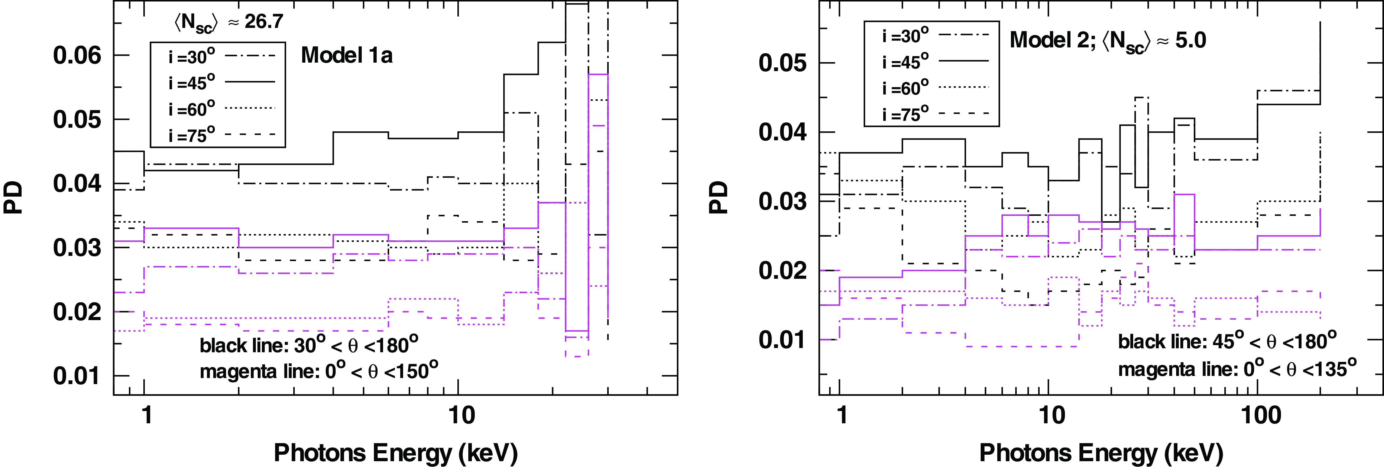
Figure 14. To understand the geometry affect in PD calculations, for simplicity we ad-hocly consider an asymmetric range of the scattering angle. The black and magenta curves are, in left panel for $\theta$ $\equiv$
[30,180
$\equiv$
[30,180 $^{\circ}$
] and [0,150
$^{\circ}$
] and [0,150 $^{\circ}$
] and in right panel for
$^{\circ}$
] and in right panel for $\theta$ $\equiv$
[45,180
$\equiv$
[45,180 $^{\circ}$
] and [0,135
$^{\circ}$
] and [0,135 $^{\circ}$
], respectively. The left and right panels are for Model 1a with
$^{\circ}$
], respectively. The left and right panels are for Model 1a with $\langle N_{sc}\rangle\approx 26.7$
and Model 2 with
$\langle N_{sc}\rangle\approx 26.7$
and Model 2 with $\langle N_{sc}\rangle\approx 5.0$
, respectively. PD is computed for four i values = 30, 45, 60, and 75 degree, and shown by dashed-dotted, solid, dotted, and dashed lines, respectively. For left panel the energy bins are same as Fig. 9 while Fig. 12 for right panel.
$\langle N_{sc}\rangle\approx 5.0$
, respectively. PD is computed for four i values = 30, 45, 60, and 75 degree, and shown by dashed-dotted, solid, dotted, and dashed lines, respectively. For left panel the energy bins are same as Fig. 9 while Fig. 12 for right panel.
7.4. Comparison with observations
In this section, we briefly discuss the polarisation properties of a few sources observed by IXPE. However, these explanation would be a purely qualitative, as we have a simple spherical corona geometry, and also the present calculations have not been implemented in the general relativity formalism. Moreover, the main motive of this exercise is to what extent one can learn in understanding of polarisation properties with having simple spherical corona geometry. We select five sources, in which two are black hole XRBs and three are neutron star XRBs.
-
4U 1630-47: IXPE had observed 4U 1630-47 from 23-Aug-2022 to 02-Sept-2022, when the source is in high soft spectral state. The polarisation properties have been analysed by three groups (Rawat et al. Reference Rawat, Garg and Méndez2023; Kushwaha et al. Reference Kushwaha, Jayasurya, Agrawal and Nandi2023; Ratheesh et al. Reference Ratheesh2023), and they found that PD is an energy-dependent which increases significantly with energy. In 2–8 keV band PD is
$\sim$
0.08 and PA in the sky plane is
$\sim$
18
$^{\circ}$
. They argue that the observations can explain in thin accretion disc with mildly relativistic outflowing medium.In the present scenario, the observed flux is described almost by Model 1a with
$\langle N_{sc}\rangle$
= 1.1 (see left upper panel of Fig. 9). Therefore, PD is energy-independent and PD = 0.08 for i = 75
$^{\circ}$
. PA is always around 90
$^{\circ}$
, that is, the electric vector is parallel to the (x-y) plane or accretion disc. The energy dependency of PD can be arose by fresh scattering in optically thin (
$\langle N_{sc}\rangle$
= 1) medium (possibly, wind) where large fraction of high-energy photons experience scattering in comparison to the low-energy photons, which will increase the PD value to 0.1 for high-energy photons (see Table 3 and text). -
Cyg X-2: Farinelli et al. (Reference Farinelli2023) measure the polarisation properties of Cyg X-2 (a Z-source), in 2–8 keV band the PD = 0.018 and PA = 140
$^{\circ}$
where the polarisation is in the direction of radio jet (possibly on the sky plane). They argue that the observed PD cannot be explained with accretion disc geometry and suggest another geometry related to the neutron star surface. The observed flux of Cyg X-2 can be described nearly with Model 1a and
$\langle N_{sc}\rangle$
=26.7. Thus for the inclination angle i
$\approx$
60
$^{\circ}$
, PD
$\approx$
0.015 and PA
$\approx$
120
$^{\circ}$
; here, we remind that PA is measured in a perpendicular plane to the escaped photon direction. Hence, our calculation indicates that the observed PD can be explained, in general, with accretion disc + corona geometry.The similar range of PD (
$\approx$
0.017) is measured for atoll source GX 9+9: by Chatterjee et al. (Reference Chatterjee, Agrawal, Jayasurya and Katoch2023). The reported PA is
$\sim$
63
$^{\circ}$
where the range of i is 40
$ -$
60
$^{\circ}$
. The observed flux can be described here by Model 1a with
$\langle N_{sc}\rangle$
lies in range 5–26. In our calculations, like Cyg X-2, the observed PD of GX 9+9 can be described in the accretion disc scenario. The calculated PA is around either (90–120
$^{\circ}$
) or (60–90
$^{\circ}$
) for a given range of i (here, 180
$^{\circ}$
differences in PA is due to the two possible definitions for modulation curve, see equation (16)). -
XTE J1701-462: IXPE had observed XTE J1701-462 during an outburst two times, Sept-2022 (epoch 1) and Oct-2022 (epoch 2). Jayasurya et al. (Reference Jayasurya, Agrawal and Chatterjee2023) measure a significant PD
$\sim$
0.045 for epoch 1 and a negligible PD
$< $
0.01 for epoch 2 in 2–8 keV band. The PA is
$\sim$
143
$^{\circ}$
, while the source has i close to 70
$^{\circ}$
. The observed flux can be described with Model 1a with
$\langle N_{sc}\rangle$
$>$
26 for epoch 1 while
$\sim$
25 for epoch 2 (see Fig. B1 for epoch 1 modeled flux). In present study with simplistic spherical geometry we can not explain the observed PD for epoch 1, one needs other geometry. However, if we exclude some fraction of forward directed escaped photons in this geometry, then we can explain the observed magnitude, see left panel of Fig. 14. Moreover the observed PD for epoch 2 can be explained in present study for
$i \sim$
70
$^{\circ}$
. The calculated PA for
$i \sim$
70
$^{\circ}$
is around 150
$^{\circ}$
. Therefore, in present observations, the polarisation properties of XTE J1701-462 indicates that the corona geometry changes in month scale. For a spectro-polarimatric study in details, we consider this source, see Appendix B. -
Cyg X-1: Krawczynski et al. (Reference Krawczynski2022) estimate the polarisation properties for hard state of Cyg X-1, the reported magnitude is PD
$\approx$
0.04 and PA
$\approx$
20
$^{\circ}$
in the plane of sky. They also find that the X-ray polarisation almost aligns with radio jet in the plane of sky, which is consistent with the previous results of Chauvin et al. (Reference Chauvin2018) using the PoGO+ balloon-borne polarimeter in 19–181 keV. Chauvin et al. (Reference Chauvin2018) had measured PD
$\approx$
0.045 and PA = 154
$^{\circ}$
in 19–181 keV. The observed flux can be described by Model 2 with
$\langle N_{sc}\rangle$
$\approx$
5, thus the estimated PD
$<$
0.025. Krawczynski et al. (Reference Krawczynski2022) found the PD
$<$
0.03 for a spherical lamp-post corona and non-spinning black hole. Therefore, our calculations are consistent with the result of Krawczynski et al. (Reference Krawczynski2022). Although, Krawczynski et al. (Reference Krawczynski2022) argue that the observed high PD can be explained with sandwich corona with i
$\sim$
45
$^{\circ}$
(see theirs Fig. 3).Clearly, like epoch 1 of XTE J1701-462, in present study with having spherical corona we can not explain the observed high PD. However, if we exclude the some fraction of forward escaped photons in spherical geometry then we can explain the observed high PD in broad band 2–181 keV (see right panel of Fig. 14).


8. Summary and conclusions
The polarisation measurement provides two independent variables, the degree of polarisation PD and the angle of polarisation PA. We observe a linearly polarised high energy emission (X-ray) in XRBs, AGNs. The observed polarisation along with spectra, and time variability may remove the existing degeneracy among theoretical models mainly in terms of the radiative process and the geometry of the emission region. We explore the linear/plane polarisation properties in the Comptonization process using a MC scheme with spherical corona geometry. We revisit the theory of polarisation in the Compton scattering process with unpolarised electrons. We argue that the $(k \times k^{\prime})$
-coordinate (in which,
$(k \times k^{\prime})$
-coordinate (in which, $(k \times k^{\prime})$
acts as a z-axis) is more suitable to describe the polarisation formalism. The single scattered unpolarised (incident) photon is polarised in perpendicular to the scattering plane. In Thomson regime, it is completely polarised for scattering angle
$(k \times k^{\prime})$
acts as a z-axis) is more suitable to describe the polarisation formalism. The single scattered unpolarised (incident) photon is polarised in perpendicular to the scattering plane. In Thomson regime, it is completely polarised for scattering angle $\theta$
= 90
$\theta$
= 90 $^{\circ}$
, see equation (7) for PD as a function of
$^{\circ}$
, see equation (7) for PD as a function of $\theta$
. The PD and PA can also be extracted for a given
$\theta$
. The PD and PA can also be extracted for a given $\theta$
from its modulation curve, see equation (8). The cross section for completely polarised incident photons of polarisation angle
$\theta$
from its modulation curve, see equation (8). The cross section for completely polarised incident photons of polarisation angle $\phi$
(or,
$\phi$
(or, $\theta_e$
), expressed by equation (10), is not an exact expression (see the Fig. 4 for deviation and validation of the approximation). The completely polarised low-energy incident photon with
$\theta_e$
), expressed by equation (10), is not an exact expression (see the Fig. 4 for deviation and validation of the approximation). The completely polarised low-energy incident photon with $\phi$
= 0 and 90
$\phi$
= 0 and 90 $^{\circ}$
retains its own polarisation properties after scattering, the PD as a function of
$^{\circ}$
retains its own polarisation properties after scattering, the PD as a function of $\theta$
after single scattering is expressed by equation (12) for a given
$\theta$
after single scattering is expressed by equation (12) for a given $\phi$
. The Stokes parameters are invariant under Lorentz transformations, particularly in Compton scattering we argue that the value of PD and PA do not change after transforming one frame to any Lorentz-boosted frame.
$\phi$
. The Stokes parameters are invariant under Lorentz transformations, particularly in Compton scattering we argue that the value of PD and PA do not change after transforming one frame to any Lorentz-boosted frame.
For $\theta$
= 0, we find that the modulation curve of scattered photon exhibits same polaris3ation characteristic of incident photon, it is also valid for the range of
$\theta$
= 0, we find that the modulation curve of scattered photon exhibits same polaris3ation characteristic of incident photon, it is also valid for the range of $\theta$ $\equiv$
[0,25
$\equiv$
[0,25 $^{\circ}$
]. We use this property to estimate the PD and PA of scattered photons with average scattering number
$^{\circ}$
]. We use this property to estimate the PD and PA of scattered photons with average scattering number $\langle N_{sc}\rangle$
, by computing the modulation curve of scattered photons of
$\langle N_{sc}\rangle$
, by computing the modulation curve of scattered photons of $\langle N_{sc} + 1\rangle$
scattering at
$\langle N_{sc} + 1\rangle$
scattering at $\theta = 0$
. We also compute directly the PD and PA of
$\theta = 0$
. We also compute directly the PD and PA of $\langle N_{sc}\rangle$
th scattered photons by using the pdf (corresponding to the cross section at
$\langle N_{sc}\rangle$
th scattered photons by using the pdf (corresponding to the cross section at $\theta = 0$
, see equation 17) for known
$\theta = 0$
, see equation 17) for known $\theta_e$
angle of
$\theta_e$
angle of $\langle N_{sc}+1\rangle$
th scattering. Interestingly, we find that for a fixed incident photon (k) direction and
$\langle N_{sc}+1\rangle$
th scattering. Interestingly, we find that for a fixed incident photon (k) direction and $\theta$ $\equiv$
[0,25
$\equiv$
[0,25 $^{\circ}$
] the distribution of projection of
$^{\circ}$
] the distribution of projection of $k^{\prime}_{e}$
(electric vector of scattered photon) on perpendicular plane to the k also reveals the polarisation properties of incident photon, which can be a working principle for Compton scattering based detector of polarisation. We write an expression (equation 18) for the resultant PD and PA of photons in particular direction which are a mixture of nth type of photons of different PD and PA.
$k^{\prime}_{e}$
(electric vector of scattered photon) on perpendicular plane to the k also reveals the polarisation properties of incident photon, which can be a working principle for Compton scattering based detector of polarisation. We write an expression (equation 18) for the resultant PD and PA of photons in particular direction which are a mixture of nth type of photons of different PD and PA.
Chandrasekhar (Reference Chandrasekhar1946) has solved the radiative transfer equations, governed by scattering opacity by free electrons, for the two states of polarisation one is along the meridian plane and another one is normal to it. It is found that the emergent photons from a given meridian plane are polarised normal to the meridian plane and PD varies zero (at i = 0) to 0.11 (at i =90 $^{\circ}$
, i: disc inclination angle). We obtain these results using the MC scheme in a step wise way after single scattering by discussing four relevant cases for unpolarised incident photons. We derive these results with considering a semi spherical corona in which seed photons source situated at the centre. The different steps involved are, case I: the incident photons are along the z-axis (i.e.
$^{\circ}$
, i: disc inclination angle). We obtain these results using the MC scheme in a step wise way after single scattering by discussing four relevant cases for unpolarised incident photons. We derive these results with considering a semi spherical corona in which seed photons source situated at the centre. The different steps involved are, case I: the incident photons are along the z-axis (i.e. $\theta_i$
= 0) and the scattering plane is fixed to the considered emergent meridian plane; case III: the incident photon direction is fixed, say (
$\theta_i$
= 0) and the scattering plane is fixed to the considered emergent meridian plane; case III: the incident photon direction is fixed, say ( $\theta_i$
,
$\theta_i$
, $\phi_i$
) and all possible scattering planes are considered; case IV: the incident photon lies on the surface of cone of opening angle
$\phi_i$
) and all possible scattering planes are considered; case IV: the incident photon lies on the surface of cone of opening angle $\theta_i$
with having all possible scattering planes; and last a general case, Case V. In particular the case IV may be relevant for the external Comptonization in blazars of radio jet of opening angle
$\theta_i$
with having all possible scattering planes; and last a general case, Case V. In particular the case IV may be relevant for the external Comptonization in blazars of radio jet of opening angle $\theta_i$
(Kumar & Kushwaha Reference Kumar and Kushwaha2021), for example, here for
$\theta_i$
(Kumar & Kushwaha Reference Kumar and Kushwaha2021), for example, here for $\theta_i$
= 15
$\theta_i$
= 15 $^{\circ}$
the maximum emergent photons escape with
$^{\circ}$
the maximum emergent photons escape with $\theta_s$ $\sim$
25
$\sim$
25 $^{\circ}$
and have PD
$^{\circ}$
and have PD $\sim$
0.06.
$\sim$
0.06.
In Thomson regime for the unpolarised incident photons, the maximum PD in general case V (or law of darkening of Chandrasekhar Reference Chandrasekhar1946) is $\sim$
0.11. However, for a fixed scattering plane and isotropic directions of k, the PD is
$\sim$
0.11. However, for a fixed scattering plane and isotropic directions of k, the PD is $\sim$
0.33 (see case I with
$\sim$
0.33 (see case I with $\theta_i \equiv [0,\pi]$
, also right panel of Fig. 3). In case of multi scattering we notice that after scattering number
$\theta_i \equiv [0,\pi]$
, also right panel of Fig. 3). In case of multi scattering we notice that after scattering number $>$
4, the maximum PD reduces to 0.02–0.035 for all discussed cases. Here, it is noted that this multi scattered photon is basically an unpolarised photon if these photons scatter freshly with optically thin medium
$>$
4, the maximum PD reduces to 0.02–0.035 for all discussed cases. Here, it is noted that this multi scattered photon is basically an unpolarised photon if these photons scatter freshly with optically thin medium $\langle N_{sc}\rangle \sim 1$
then the PD as a function of i is again described by Table 3.
$\langle N_{sc}\rangle \sim 1$
then the PD as a function of i is again described by Table 3.
We explore the energy dependency of polarisation for unpolarised incident photons by considering mainly two different spectral sets of parameters corresponding to the hard (larger electron medium temperature, $kT_e$
= 100 keV) and soft (
$kT_e$
= 100 keV) and soft ( $kT_e$
= 2.5 keV) states. For calculations, we take a simple spherical corona geometry and estimate the polarisation of scattered photons with two average scattering numbers
$kT_e$
= 2.5 keV) states. For calculations, we take a simple spherical corona geometry and estimate the polarisation of scattered photons with two average scattering numbers $\langle N_{sc}\rangle$ $\sim$
1.1 and 5 for each spectral set. We compute for four inclination angles of disc i =
$\sim$
1.1 and 5 for each spectral set. We compute for four inclination angles of disc i = $\theta_s$
= 30
$\theta_s$
= 30 $^{\circ}$
, 45
$^{\circ}$
, 45 $^{\circ}$
, 60
$^{\circ}$
, 60 $^{\circ}$
, and 75
$^{\circ}$
, and 75 $^{\circ}$
; here, we have considered the (x,y)-plane as an accretion disc. With spherical corona geometry, we find that the PD is independent of seed photon source temperature
$^{\circ}$
; here, we have considered the (x,y)-plane as an accretion disc. With spherical corona geometry, we find that the PD is independent of seed photon source temperature $kT_b$
, and for
$kT_b$
, and for $\langle N_{sc}\rangle$ $\sim$
1.1 the PD is independent of energy in 2–8 keV band for both spectral sets. Since, in Thomson regime the Comptonized flux is independent of
$\sim$
1.1 the PD is independent of energy in 2–8 keV band for both spectral sets. Since, in Thomson regime the Comptonized flux is independent of $\theta$
, thus for the unpolarised incident photons and non-relativistic corona temperature, the PD of the scattered photons would be independent of E (see Appendix B) atleast after single scattering. The magnitude of PD as a function of i is slightly lower than the values listed in Table 3 for
$\theta$
, thus for the unpolarised incident photons and non-relativistic corona temperature, the PD of the scattered photons would be independent of E (see Appendix B) atleast after single scattering. The magnitude of PD as a function of i is slightly lower than the values listed in Table 3 for $\langle N_{sc}\rangle$ $\sim$
1.1 as expected. For
$\sim$
1.1 as expected. For $\langle N_{sc}\rangle$ $\sim$
5, the maximum value of PD is
$\sim$
5, the maximum value of PD is $\sim$
0.03 at
$\sim$
0.03 at $i = 45^{\circ}$
. In present convention, PA =
$i = 45^{\circ}$
. In present convention, PA = $90^{\circ}$
means that the electric vector is parallel to the accretion disc (or (x,y)-plane) for all i. We find that for both spectral sets with
$90^{\circ}$
means that the electric vector is parallel to the accretion disc (or (x,y)-plane) for all i. We find that for both spectral sets with $\langle N_{sc}\rangle$ $\sim$
1.1 the PA is
$\sim$
1.1 the PA is $\sim$ $90^{\circ}$
while for
$90^{\circ}$
while for $\langle N_{sc}\rangle$ $\sim$
5, the PA at
$\sim$
5, the PA at $i=75^{\circ}$
is
$i=75^{\circ}$
is $\sim$
120
$\sim$
120 $^{\circ}$
and 140
$^{\circ}$
and 140 $^{\circ}$
for soft and hard spectral sets, respectively.
$^{\circ}$
for soft and hard spectral sets, respectively.
We also estimate the polarisation for Wien spectra for both spectral sets. We find that in Thomson regime PD has maximum value $\sim$
0.03 at i=45
$\sim$
0.03 at i=45 $^{\circ}$
. Since the emergent photons spectra from thin disc are a black body mainly due to the large optical depth governed by Thomson scattering (e.g. Shakura & Sunyaev Reference Shakura and Sunyaev1973, see also Kumar & Mukhopadhyay Reference Kumar and Mukhopadhyay2021). Thus, these Wien spectra calculations indicate that the polarisation of emergent photons from the thin disc will not be described by Table 3, but it has maximum value
$^{\circ}$
. Since the emergent photons spectra from thin disc are a black body mainly due to the large optical depth governed by Thomson scattering (e.g. Shakura & Sunyaev Reference Shakura and Sunyaev1973, see also Kumar & Mukhopadhyay Reference Kumar and Mukhopadhyay2021). Thus, these Wien spectra calculations indicate that the polarisation of emergent photons from the thin disc will not be described by Table 3, but it has maximum value $\sim$
0.03 for i=45
$\sim$
0.03 for i=45 $^{\circ}$
, see also Fig. 13.
$^{\circ}$
, see also Fig. 13.
Recently, IXPE has observed many XRBs and AGNs sources and the estimated PD for few sources is larger than 0.03, which can not be explained with considered simple spherical geometry. To understand the geometry dependency for polarisation within this, we ad-hocly exclude the some range of the scattering angle. For a soft spectral set we obtain PD $\sim$
0.045 at
$\sim$
0.045 at $i = 45^{\circ}$
with
$i = 45^{\circ}$
with $\theta$
range [30,180
$\theta$
range [30,180 $^{\circ}$
], and so we qualitatively obtain the observed PD value for source XTE J1701-462 (Jayasurya et al. Reference Jayasurya, Agrawal and Chatterjee2023). Similarly, to explain the observed PD (
$^{\circ}$
], and so we qualitatively obtain the observed PD value for source XTE J1701-462 (Jayasurya et al. Reference Jayasurya, Agrawal and Chatterjee2023). Similarly, to explain the observed PD ( $\sim$
0.04) for Cyg X-1, Krawczynski et al. (Reference Krawczynski2022) conclude that it can not be obtained with simple spherical corona, which is consistent with our conclusions. We qualitatively understand the estimated polarisation properties for five sources observed by IXPE within spherical corona geometry, and we almost align with the author’s conclusions, except a few. In future, we intend to study the polarisation properties with proper geometries of corona and also with implementation of general relativity formalism in MC scheme.
$\sim$
0.04) for Cyg X-1, Krawczynski et al. (Reference Krawczynski2022) conclude that it can not be obtained with simple spherical corona, which is consistent with our conclusions. We qualitatively understand the estimated polarisation properties for five sources observed by IXPE within spherical corona geometry, and we almost align with the author’s conclusions, except a few. In future, we intend to study the polarisation properties with proper geometries of corona and also with implementation of general relativity formalism in MC scheme.
Acknowledgements
We thank the referee for their comments and suggestions that have improved the presentation of the paper. The work is partly supported by the Dr. D. S. Kothari Post-Doctoral Fellowship (201718-PH/17-18/0013) of University Grant Commission (UGC), New Delhi.
Data availability
In Fig. B1, the data is taken from published work of Jayasurya et al. (Reference Jayasurya, Agrawal and Chatterjee2023).
A.
$\langle U \rangle$
and
$\langle Q \rangle $
for polarised incident photons


Fig. A1 shows the Stokes parameters U and Q as a function of scattering angle (see Section 2.2 for the expression) for three different values of polarisation angle of polarised (incident) photons $\phi$
= 30, 45, and 60
$\phi$
= 30, 45, and 60 $^{\circ}$
. Here, one can notice that for a small range of
$^{\circ}$
. Here, one can notice that for a small range of $\theta$
the U dominates over Q. However, for all cases we find that
$\theta$
the U dominates over Q. However, for all cases we find that $\langle U \rangle$ $<<$
$<<$ $\langle Q \rangle$
.
$\langle Q \rangle$
.
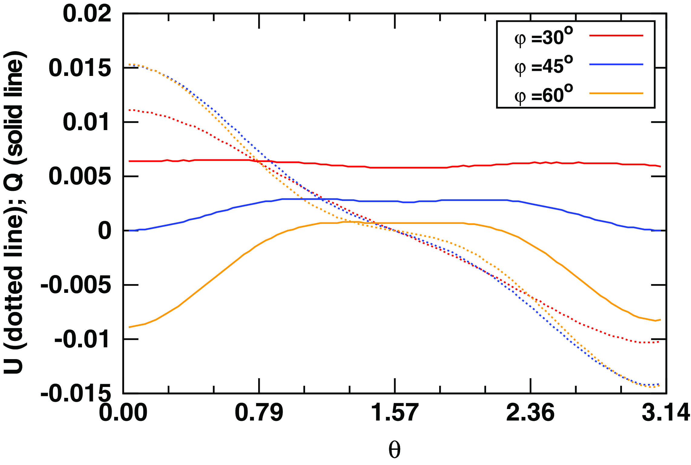
Figure A1. $U (\propto \sin 2\phi \cos \theta)$
and
$U (\propto \sin 2\phi \cos \theta)$
and $Q (\propto (\cos^2\phi -\sin^2\phi\cos^2\theta))$
of the single scattered polarised (incident) photons as a function of
$Q (\propto (\cos^2\phi -\sin^2\phi\cos^2\theta))$
of the single scattered polarised (incident) photons as a function of $\theta$
. The dotted and solid curves are for U and Q, respectively. The red, blue, and orange curves are for
$\theta$
. The dotted and solid curves are for U and Q, respectively. The red, blue, and orange curves are for $\phi$
= 30, 45, and 60
$\phi$
= 30, 45, and 60 $^{\circ}$
, respectively.
$^{\circ}$
, respectively.
B. XTE J1701-462: Spectro-polarimatric comparision
For a observed spectro-polarimatric comparision we consider the source XTE J1701-462. The data points for flux are taken from Jayasurya et al. (Reference Jayasurya, Agrawal and Chatterjee2023, see theirs Figure 3). Unlike the detail modeling of Jayasurya et al. (Reference Jayasurya, Agrawal and Chatterjee2023), we describe the observed flux by Comptonization only, with aiming to estimate the polarisation properties. The result for flux modeling in spherical geometry is shown in the upper panel of Fig. B1, and the model parameters are $kT_e$
= 2.5 keV;
$kT_e$
= 2.5 keV; $kT_b$
= 1.25 keV;
$kT_b$
= 1.25 keV; $\langle N_{sc}\rangle$
= 24.7. We compute the PD as a function of E for two different ranges of
$\langle N_{sc}\rangle$
= 24.7. We compute the PD as a function of E for two different ranges of $\theta$ $\equiv$
[0, 180
$\equiv$
[0, 180 $^{\circ}$
] and [45, 180
$^{\circ}$
] and [45, 180 $^{\circ}$
], which is shown in the middle and lower panels of Fig. B1, respectively. We find that the variation of PA with energy is similar to the case Model Ia with
$^{\circ}$
], which is shown in the middle and lower panels of Fig. B1, respectively. We find that the variation of PA with energy is similar to the case Model Ia with $\langle N_{sc}\rangle$
= 26.7. As noted earlier the observed PD of epoch 1 can not be explained in the spherical corona geometry, but one needs a different geometry where the
$\langle N_{sc}\rangle$
= 26.7. As noted earlier the observed PD of epoch 1 can not be explained in the spherical corona geometry, but one needs a different geometry where the $\theta$
-angle distribution of escaped Comptonized photons does not follow the same variation as shown in Fig. 10. We also here noted that for both ranges of
$\theta$
-angle distribution of escaped Comptonized photons does not follow the same variation as shown in Fig. 10. We also here noted that for both ranges of $\theta$
the computed fluxes are same. This is because of that in Thomson regime the scattered frequency does not depends on
$\theta$
the computed fluxes are same. This is because of that in Thomson regime the scattered frequency does not depends on $\theta$
but only on angle
$\theta$
but only on angle $\alpha$
and
$\alpha$
and $\alpha'$
, where
$\alpha'$
, where $\alpha$
is the angle between incident photon and incident electron,
$\alpha$
is the angle between incident photon and incident electron, $\alpha'$
is the angle between scattered photon and incident electron, and in the lab frame it is determined as
$\alpha'$
is the angle between scattered photon and incident electron, and in the lab frame it is determined as $\frac{\nu'}{\nu} = \frac{1-\frac{\text v}{c}\cos \alpha}{1-\frac{\text v}{c}\cos \alpha'+\frac{h\nu}{\gamma m_e c^2} (1-\cos \theta)}$
. Hence, in general, in Thomson regime the Comptonized flux is independent of
$\frac{\nu'}{\nu} = \frac{1-\frac{\text v}{c}\cos \alpha}{1-\frac{\text v}{c}\cos \alpha'+\frac{h\nu}{\gamma m_e c^2} (1-\cos \theta)}$
. Hence, in general, in Thomson regime the Comptonized flux is independent of $\theta$
. Further in Thomson regime and non-relativistic corona temperature, for unpolarised incident photons, the PD of the scattered photons would be independent of E atleast after single scattering (as noted), since the PD as a function of
$\theta$
. Further in Thomson regime and non-relativistic corona temperature, for unpolarised incident photons, the PD of the scattered photons would be independent of E atleast after single scattering (as noted), since the PD as a function of $\theta$
is described by curve 1 of Fig. 2.
$\theta$
is described by curve 1 of Fig. 2.

Figure B1. Spectro-polarimatric measurement for source XTE J1701-462 in spherical corona. The upper panel is for the flux, here the data points are taken from Jayasurya et al. (Reference Jayasurya, Agrawal and Chatterjee2023), the solid curve is for Comptonized flux, the dotted curve is for seed black body flux, and the dashed curve is Comptonized flux having different $\theta$
range [45, 180
$\theta$
range [45, 180 $^{\circ}$
]. The parameters for Comptonization are
$^{\circ}$
]. The parameters for Comptonization are $kT_e$
= 2.5 keV;
$kT_e$
= 2.5 keV; $kT_b$
= 1.25 keV;
$kT_b$
= 1.25 keV; $\langle N_{sc}\rangle$
= 24.7. The middle and lower panels are for PD with having
$\langle N_{sc}\rangle$
= 24.7. The middle and lower panels are for PD with having $\theta$
range [0,180
$\theta$
range [0,180 $^{\circ}$
] and [45, 180
$^{\circ}$
] and [45, 180 $^{\circ}$
], respectively.
$^{\circ}$
], respectively.


