


1. Introduction
Thermal convection, occurring in fluid that is heated from below and subjected to sufficiently large temperature gradients, is ubiquitous and takes on a great importance in nature and industrial processes (Ahlers, Grossmann & Lohse Reference Ahlers, Grossmann and Lohse2009; Lohse & Xia Reference Lohse and Xia2010), for example, atmospheric and oceanic circulation, mantle and core convection, convective flows occurring in metal-production and crystal-growth processes, etc. For practical uses, turbulent thermal convection can be beneficial to the efficient heat transport but highly fluctuating temperature might also be detrimental to some applications. Most previous efforts have focused on the beneficial purposes, e.g. the enhancement of convective heat transfer is helpful for heat exchangers, material mixing and chemical reaction (Wang, Mathai & Sun Reference Wang, Mathai and Sun2019). Many effective approaches have been proposed to enhance heat transport, such as imposing oscillatory flow pulsation (Piccolo et al. Reference Piccolo, Siclari, Rando and Cannistraro2017; Wu et al. Reference Wu, Dong, Wang and Zhou2021), applying wall roughness (Zhu et al. Reference Zhu, Stevens, Verzicco and Lohse2017; Emran & Shishkina Reference Emran and Shishkina2020; Yang et al. Reference Yang, Zhang, Jin, Dong, Wang and Zhou2021), introducing wall temperature oscillation (Yang et al. Reference Yang, Chong, Wang, Verzicco, Shishkina and Lohse2020; Zhao et al. Reference Zhao, Wang, Wu, Chong and Zhou2022a,Reference Zhao, Zhang, Wang, Wu, Chong and Zhoub), adding the shear effects (Blass et al. Reference Blass, Zhu, Verzicco, Lohse and Stevens2020; Jin et al. Reference Jin, Wu, Zhang, Liu and Zhou2022) and using the multiphase turbulence (Biferale et al. Reference Biferale, Perlekar, Sbragaglia and Toschi2012; Wang et al. Reference Wang, Mathai and Sun2019; Liu et al. Reference Liu, Chong, Ng, Verzicco and Lohse2022; Yang et al. Reference Yang, Zhang, Wang, Dong and Zhou2022). However, few attentions have been paid on the possible detrimental aspects caused by thermal convection. Examples include the occurrence of thermal convection during crystal growth that adversely affects the quality of the crystal (Heijna et al. Reference Heijna, Poodt, Tsukamoto, De Grip, Christianen, Maan, Hendrix, Van Enckevort and Vlieg2007); the presence of parasitic convection in thermoacoustic devices and cryocoolers that not only brings a deleterious effect on the desired operation but also decreases the thermodynamic efficiency (Ross Jr. & Johnson Reference Ross and Johnson2004). Hence, strategies to suppress thermal convection are particularly important to both scientific and industrial communities (Chong et al. Reference Chong, Yang, Huang, Zhong, Stevens, Verzicco, Lohse and Xia2017; Jiang et al. Reference Jiang, Zhu, Mathai, Verzicco, Lohse and Sun2018).
Mechanical vibration is ubiquitous and inevitable in almost all industrial applications. Thermal convection under the action of vibration is called thermal vibrational convection (TVC) (Gershuni & Lyubimov Reference Gershuni and Lyubimov1998). Earlier studies on TVC discovered that vibration creates an ‘artificial gravity’ to operate fluids (Beysens et al. Reference Beysens, Chatain, Evesque and Garrabos2005; Beysens Reference Beysens2006), and provides one possible way to trigger thermal instability under microgravity conditions (Mialdun et al. Reference Mialdun, Ryzhkov, Melnikov and Shevtsova2008; Shevtsova et al. Reference Shevtsova, Ryzhkov, Melnikov, Gaponenko and Mialdun2010). Most previous works have focused on the investigation of TVC at low Rayleigh numbers, for instance, the vibrational effect on the flow pattern slightly beyond the critical Rayleigh number (Clever, Schubert & Busse Reference Clever, Schubert and Busse1993; Rogers et al. Reference Rogers, Schatz, Bougie and Swift2000a,Reference Rogers, Schatz, Brausch and Peschb) and the influence of vibration on the critical Rayleigh number of thermal instability (Cissé, Bardan & Mojtabi Reference Cissé, Bardan and Mojtabi2004; Lappa Reference Lappa2009; Carbo, Smith & Poese Reference Carbo, Smith and Poese2014; Swaminathan et al. Reference Swaminathan, Garrett, Poese and Smith2018; Kozlov, Rysin & Vjatkin Reference Kozlov, Rysin and Vjatkin2019). It is concluded that high-frequency vibration can prepone or postpone the onset of buoyancy-driven convective instability, depending on the relative direction of vibration to the temperature gradient (Pesch et al. Reference Pesch, Palaniappan, Tao and Busse2008; Lappa Reference Lappa2016; Bouarab et al. Reference Bouarab, Mokhtari, Kaddeche, Henry, Botton and Medelfef2019). A few works are related to the influences of vertical vibrations on heat transfer at low Rayleigh numbers (Lyubimova et al. Reference Lyubimova, Lizee, Gershuni, Lyubimov, Chen, Wadih and Roux1994; Zidi, Hasseine & Moummi Reference Zidi, Hasseine and Moummi2018). Recently, it was discovered that due to the vibration-induced destabilization effects, translational vibration can achieve a dramatic enhancement of the convective heat-transfer rate in the turbulent regime (Wang, Zhou & Sun Reference Wang, Zhou and Sun2020; Guo et al. Reference Guo, Wang, Wu, Chong and Zhou2022). Moreover, the Rayleigh–Taylor turbulence in the zero-gravity condition is found to be suppressed after long-time development under the action of the time-periodic vibration (Boffetta, Magnani & Musacchio Reference Boffetta, Magnani and Musacchio2019).
The influence of high-frequency vibrations on the onset criteria of convection, flow pattern and heat transport at low Rayleigh numbers has been studied in past decades. Although Wang et al. (Reference Wang, Zhou and Sun2020), Guo et al. (Reference Guo, Wang, Wu, Chong and Zhou2022) and Boffetta et al. (Reference Boffetta, Magnani and Musacchio2019) have extended to high Rayleigh numbers in recent years, those studies only concern the destabilizing effect of the translational vibration (perpendicular to the direction of the temperature gradient) on buoyancy-driven convection under terrestrial conditions, or the stabilizing effect of vertical vibration (parallel to the direction of the temperature gradient) on thermal convection under zero-gravity conditions. However, in the terrestrial environment with the influence of gravity, whether the dynamical stabilization by vertical vibration can be extended to the high-Rayleigh-number regime is still unknown, how vertical vibration affects thermal convection in the turbulent regime has not been systematically explored before, and the mechanism involved is still mysterious. The present investigation will unveil the physical mechanism for vibration-induced taming thermal turbulence at high Rayleigh numbers and shed light on the influences of vertical vibration on the characteristics of turbulent structures and heat transport. In this paper we choose the paradigm of thermal turbulence – Rayleigh–Bénard (RB) turbulence in a cubic cell and investigate how vertical vibration tames turbulent heat transport. In § 2 governing equations and the numerical approach of RB convection with vertical vibration are described. In § 3.1 vibration-induced suppression of heat transport and convective flow intensity is observed and analysed. In § 3.2 the vibrational influence on the time series of the Nusselt and Reynolds numbers is investigated, and the amplitude response is shown. In § 3.3 the vibrational effects on the mean flow and scaling relations are studied. In § 3.4, with taking thermally led gravitational and the vibration-induced anti-gravitational effects, we proposed an effective Rayleigh number, and then extended the Grossmann–Lohse (GL) theory to predict the reduction on the heat-transport and flow intensity. In § 4 the non-uniformity of vibration-induced ‘anti-gravity’ is studied. Finally, the conclusion is given in § 5.
2. Numerical methods
In the present study we account for turbulent RB convection in a cubic cell. Vertical harmonic vibrations are introduced to control the heat-transport mechanism in thermal turbulence. Under the action of vertical vibration, the Oberbeck–Boussinesq equations for thermal turbulence read (Shevtsova et al. Reference Shevtsova, Ryzhkov, Melnikov, Gaponenko and Mialdun2010; Wang et al. Reference Wang, Zhou and Sun2020)
 $$\begin{gather} \boldsymbol{\nabla} \boldsymbol{\cdot} \boldsymbol{u} = 0, \end{gather}$$
 $$\begin{gather}\partial_t \boldsymbol{u} + (\boldsymbol{u} \boldsymbol{\cdot} \boldsymbol{\nabla}) \boldsymbol{u} ={-}\boldsymbol{\nabla} p + \nu \nabla^2 \boldsymbol{u} + \alpha \theta (g - A\varOmega^2 \cos(\varOmega t)) \boldsymbol{e}_3, \end{gather}$$
 $$\begin{gather}\partial_t \theta + (\boldsymbol{u} \boldsymbol{\cdot} \boldsymbol{\nabla}) \theta = \kappa \nabla^2 \theta, \end{gather}$$
where  $\boldsymbol {u}=(u_1,u_2,u_3)$ denotes the fluid velocity, $p$ the pressure, $\theta$ the temperature and $\boldsymbol {e}_3$ the unit vector in the vertical direction. In (2.1)–(2.3), taking the cell size $H$, the free-fall velocity $\sqrt {\alpha g \varDelta H}$, the temperature difference $\varDelta$ between the top and bottom plates as the characteristic length, velocity, temperature, it readily yields four dimensionless control parameters, i.e. Rayleigh number $\mbox {Ra}$, Prandtl number ${Pr}$, vibration amplitude $a$ and vibration frequency $\omega$. They are given by
 \begin{equation} {Ra} = \frac{\alpha g \varDelta H^3}{\nu \kappa}, \quad {Pr} = \frac{\nu}{\kappa}, \quad {a} = \frac{A \alpha \varDelta }{H}, \quad \omega = \sqrt{\frac{\varOmega^2 H}{\alpha g \varDelta}}, \end{equation}
where  $\alpha$ denotes the isobaric thermal expansion coefficient, $\nu$ the kinetic viscosity, $\kappa$ the thermal conductivity of the working fluid, $g$ the magnitude of gravitation, $A$ the vibration amplitude and $\varOmega$ the vibration frequency. In the limit of small amplitude and high frequency, the intensity of the vibrational source is usually quantified by the vibrational Rayleigh number $\mbox {Ra}_{vib}$, which is analogous to the Rayleigh number in thermally driven RB convection, given by
 \begin{equation} {Ra}_{vib} = \frac{(A\varOmega \alpha \varDelta H)^2}{2\nu \kappa} = \frac{{a}^2 \omega^2 {Ra}}{2} . \end{equation}
 We carried out direct numerical simulations of vertically vibrated RB turbulence in a cubic cell of size  $H=1$, as shown in figure 1(i). The Rayleigh number ranges from $\mbox {Ra} = 10^7$ to $\mbox {Ra} = 10^9$ and the dimensionless vibration frequency from $\omega = 0$ to $\omega = 700$. The Prandtl number is fixed at ${Pr} = 4.38$ and the dimensionless amplitude fixed at ${a} = 1.52 \times 10^{-3}$, which corresponds to a small vibration amplitude $A = 0.1 H$, and the working fluid of water at $40\,^\circ$C in the experiment. We choose the small amplitude and high frequency (compared with the viscous diffusion time scale), as this kind of vibration is omnipresent in nature and industrial applications, and the condition of small amplitude and high frequency will be used in § 3.4. The governing equations (2.1)–(2.3) are numerically solved by the Nek5000 spectral element method package, which has been well validated in the literature (Chandra & Verma Reference Chandra and Verma2013; Pandey, Scheel & Schumacher Reference Pandey, Scheel and Schumacher2018; Wang et al. Reference Wang, Zhou and Sun2020). At all solid boundaries, no-slip boundary conditions are applied for the velocity. At the top and bottom plates, constant temperatures $\theta _{top}=-0.5$ and $\theta _{bot}=0.5$ are given and at all sidewalls, the adiabatic conditions are adopted. For all simulations, the mesh size is chosen to adequately resolve the near-wall dynamics and small scales in bulk zones, and the time step is chosen to not only fulfil the Courant–Friedrichs–Lewy conditions, but also resolve the Kolmogorov time scale and time scale of one percent of the vibration period. For instance, at $\mbox {Ra}=10^9$ and $\omega = 700$, we set the number of spectral elements to be $128\times 128\times 128$ and the number of Gauss–Legendre–Lobatto quadrature points to be seven within each spectral element. The elements are clustered to solid surfaces to resolve the thermal and viscous boundary layers. We also carefully design the mesh to adequately resolve both the Kolmogorov length scale for the velocity field and the Batchelor length scale for the temperature field. All statistics are calculated over an averaging time of more than 400 dimensionless time units for $\omega \leq 200$ and 250 dimensionless time units for $\omega > 200$ after the system has reached the statistically steady state. More details about numerical methods can be found in our previous studies (Wang et al. Reference Wang, Zhou and Sun2020; Wu et al. Reference Wu, Dong, Wang and Zhou2021).

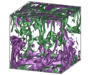
Figure 1. (a–c) Instantaneous flow structures visualized by volume rendering of temperature anomaly for various vibration frequencies  $\omega = 0, 400, 700$ at $\mbox {Ra} = 10^9$, ${Pr}=4.38$ and $a=1.52\times 10^{-3}$ (see supplementary movies 1 to 3 available at https://doi.org/10.1017/jfm.2022.850). (d–f) The corresponding temperature contours on the respective horizontal slices at $x_3 = \delta _{th}(\omega )$, where $\delta _{th}(\omega ) = H/(2 {Nu}(\omega ))$ is the thermal boundary layer (TBL) thickness. (g) Vibration-induced heat-transport suppression expressed by the ratio of Nusselt numbers ${Nu}(\omega )/{Nu}(0)$ vs $\omega$. Inset shows the heat content $Q_p(\omega )/Q_p(0)$ of hot plumes as a function of $\omega$ obtained at $x_3 = \delta _{th}(\omega )$ near the bottom plate. (h) Flow reduction expressed by the ratio of Reynolds numbers ${Re}(\omega )/{Re}(0)$ vs $\omega$. The cyan shaded area corresponds to the regime in which vibration has no or slight effects on ${Nu}$ and ${Re}$; the purple shaded area corresponds to the regime where both flow reduction and heat-transfer suppression take place. Note that the division for two regions is roughly estimated, and we will focus on the critical vibration frequency in our future studies. (i) Sketch of the cubic convection cell with the coordinate system $(x_1, x_2, x_3)$ and boundary conditions; in this coordinate system the corresponding three components of fluid velocity are expressed by $\boldsymbol {u} = (u_1, u_2, u_3)$.
3. Results and discussion
3.1. Vibration-induced heat-transport suppression
Figure 1(a–c) displays the typical instantaneous flow structures visualized by the volume rendering of temperature anomaly field ( $\theta - \langle \theta \rangle _t$) with different frequencies $\omega = 0, 400, 700$ at $\mbox {Ra} = 10^9$. Here, $\langle {\cdot }\rangle _t$ represents an average over time. For the standard RB turbulence without any vibration, as shown in figure 1(a,d), intense turbulent fluctuations distort the isotherms and massive eruptions of thermal plumes are randomly triggered from thermal boundary layers (TBLs) (Grossmann & Lohse Reference Grossmann and Lohse2004; Ahlers et al. Reference Ahlers, Grossmann and Lohse2009; van der Poel et al. Reference van der Poel, Verzicco, Grossmann and Lohse2015). Hot and cold plumes are then transported and mixed by the large-scale wind (Brown & Ahlers Reference Brown and Ahlers2007; Wei Reference Wei2021).
When vertical vibration is applied to the convection cell, as shown in figure 1(b,c,e, f), the overall eruptions of thermal plumes are obviously inhibited, and the subsequent plume fragmentation that leads to small and fragmented plumes are also suppressed. The reason is that in the presence of vertical vibration, a dynamical averaging effect of the oscillating force against gravity can be resulted (Apffel et al. Reference Apffel, Novkoski, Eddi and Fort2020), which postpones the convective instability and leads to the stabilization on turbulent convective flows and unstable thermal gradients. Hence, the action of vertical vibration attenuates the intensity of buoyancy-driven convection and stabilizes TBLs, thereby prevents thermal plumes from fragmenting by turbulent fluctuations and suppresses plume emissions. This implies that vertical vibration has the ability to tame thermal convection, even in a turbulent regime.
To quantify vibration effects on the global transport properties of thermal turbulence, we plot the ratios of the Nusselt number  ${Nu}(\omega )/{Nu}(0)$ and Reynolds number ${Re}(\omega )/{Re}(0)$ as a function of the vibration frequency $\omega$ in figure 1(g,h). The Nusselt and Reynolds numbers are defined as ${Nu} = \langle u_3 \theta - \kappa \partial _{x_3}\theta \rangle /(\kappa \varDelta /H)$ and ${Re} = U_{rms}H/\nu$, respectively, where $U_{rms} = \sqrt {\langle \boldsymbol {u} \boldsymbol {\cdot } \boldsymbol {u} \rangle }$ and $\langle \boldsymbol {\cdot }\rangle$ denotes a spatial and temporal average. We find that when the vibration frequency is small ( $\omega \lesssim 120$, the cyan shaded area of figure 1g,h), both the measured ${Nu}(\omega )$ and ${Re}(\omega )$ are close to the RB values of ${Nu}(0)$ and ${Re}(0)$, respectively. As expected, in the case of small $\omega$, the dynamical averaging effect induced by vertical vibration is too small to balance the gravity and, thus, the system resembles classical thermal turbulence. As $\omega$ increases ( $\omega \gtrsim 120$, the purple shaded area of figure 1g,h), vertical vibration leads to the significant decline of ${Nu}(\omega )/{Nu}(0)$ and ${Re}(\omega )/{Re}(0)$. This indicates that when $\omega$ is sufficiently large, vibration-induced dynamical stabilization dominates the convective flow. Therefore, one obtains the weakened large-scale wind and suppressed turbulent fluctuations, and, thus, the reduced global heat flux of the system. Furthermore, heat-transport suppression can also be quantified by the vibration-induced reduction of ‘heat’ contained in the plumes. The inset of figure 1(g) shows the heat content of hot plumes, $Q_p = \sum c_p \rho V_{grid} \theta$, obtained on the horizontal slices at $x_3 = \delta _{th}(\omega )$, where $c_p$ and $\rho$ denote the specific heat and density of the working fluid and $V_{grid}$ is the volume of each grid point, the thickness of the TBL is estimated by $\delta _{th}(\omega ) = H/[2{Nu}(\omega )]$. Here, the criterion for extracting hot plumes on horizontal slices is $\theta - \langle \theta \rangle _{h} > \theta _{rms}$ and $u_3 \theta /(\kappa \varDelta /H) > {Nu}$, where $\langle \boldsymbol {\cdot } \rangle _{h}$ means the surface averaging over horizontal slice and $\theta _{rms}$ is the root mean square of $\theta - \langle \theta \rangle _{h}$ on the slice. More details about extracting thermal plumes and calculating heat content can be found in Woods (Reference Woods2010), Huang et al. (Reference Huang, Kaczorowski, Ni and Xia2013) and Wang et al. (Reference Wang, Zhou and Sun2020). One sees clearly that the heat contained by hot plumes dramatically drops in the ${Nu}$-suppression regime.
Next, we examine the vibrational effects on the spatial distribution of heat flux. Figure 2 shows the measured local heat flux  $\langle {Nu}_l(x_1) \rangle _t$ as a function of $x_1$ at the mid-height of the cell for various $\omega$, where ${Nu}_l$ is given by
 \begin{equation} {Nu}_l = \frac{\langle u_3 {\theta}\rangle_{x_2} - \kappa \partial_{3} \langle \theta \rangle_{x_2}}{\kappa \varDelta/H}, \end{equation}
where  $\langle {\cdot } \rangle _{x_2}$ denotes an average along the $x_2$ direction at the mid-height of the cell. It is seen that, for all values of $\omega$, intense local heat flux occurs near the cell sidewalls, suggesting that heat is mainly carried upwards by the large-scale wind or thermal plumes even for the highly vibrated cases. It is also seen that both the magnitudes of the profiles in the near-side-wall regions and those in the bulk region of vertically vibrated RB convection are obviously reduced compared with that of the standard RB case, implying that vertical vibrations dampen the intensity of convective flows in all regions and then suppress convective heat transport. With increasing $\omega$ from $200$ to $700$, the value of $\langle {Nu}_l \rangle _t$ is nearly unchanged in near-side-wall regions, but significantly decreases, indicating that vibration-induced suppression is stronger at larger $\omega$.

Figure 2. Local heat-transport rate  $\langle {Nu}_l(x_1) \rangle _t$ as a function of the horizontal position $x_1$ in vertically vibrated RB convection at $\mbox {Ra} = 10^9$ for various frequencies $\omega = 0, 200, 400, 700$.
To systematically reveal the vibration effects on  ${Nu}$ and ${Re}$ numbers, we carry out a series of three-dimensional simulations of vertically vibrated RB turbulence over the Rayleigh number range from $\mbox {Ra} = 10^7$ to $\mbox {Ra} = 10^9$. Figure 3(a–e) shows the variations of ${Nu}$ normalized by the corresponding RB values (i.e. $\omega =0$) for different $\mbox {Ra}$. The ${Nu}$ reduction is rather robust, i.e. it can be observed for all $\mbox {Ra}$ studied. Specifically, the reduction is more pronounced at larger $\mbox {Ra}$ or higher $\omega$, and the reduction regimes shift towards lower $\omega$ as $\mbox {Ra}$ increases, suggesting that the reduction occurs more easily at larger $\mbox {Ra}$. Similar results for the vibration-induced suppression on ${Re}$ are also observed in figure 3( f–j).

Figure 3. Ratios (a–e)  ${Nu}(\omega )/{Nu}(0)$ and ( f–j) ${Re}(\omega )/{Re}(0)$ as a function of vibration frequency $\omega$ for various Rayleigh numbers. (a, f): ${$_{\blacksquare}$}$, black for $\mbox {Ra} = 10^7$, (b,g): ${\blacktriangle }$, red for $\mbox {Ra} = 3 \times 10^7$, (c,h): ${\bullet }$, green for $\mbox {Ra} = 10^8$, (d,i): ${\blacktriangledown }$, blue for $\mbox {Ra} = 3 \times 10^8$, (e,j): ${$_{\blacklozenge}$}$, thistle for $\mbox {Ra} = 10^9$. The solid curves represent the predictions obtained by the extended GL theory.
3.2. Time series and amplitude response of  ${Nu}$ and ${Re}$


Next, we focus on the vibrational influence on the time series of both  ${Nu}(t)$ and ${Re}(t)$. Figure 4 depicts the time series of ${Nu}(t)$ and ${Re}(t)$ in vertically vibrated RB convection at $\mbox {Ra} = 10^9$ for various frequencies $\omega = 0, 40, 200, 400, 700$. Due to the introduction of vertical vibration, the development of convective velocities oscillating with time leads to oscillatory properties of the ${Nu}$ and ${Re}$ numbers. It is shown in figures 4(b–e) and 4(g–j) that an oscillatory perturbation is added to both the ${Nu}$ and ${Re}$ time series via the imposition of vibrations. It is also seen that with increasing $\omega$, the magnitude of perturbations increases rapidly, but the time-averaged value of the ${Nu}$ and ${Re}$ time series decreases, namely, vertical vibration destabilizes the convective flows and achieves heat-transport suppression. Even at the highest frequency $\omega = 700$ the negative global heat transport happens at a certain time, as shown in figure 4(e).

Figure 4. Time series of (a–e)  ${Nu}$ and ( f–j) ${Re}$ in vertically vibrated thermal turbulence at $\mbox {Ra}=10^9$ and ${Pr}=4.38$ for various frequencies (a, f) $\omega = 0$, (b,g) $\omega = 40$, (c,h) $\omega = 200$, (d,i) $\omega = 400$ and (e,j) $\omega = 700$. The insets show the time series of ${Nu}$ and ${Re}$ within six vibration periods started from $t=300$. The $x$ coordinate in each inset is scaled by the vibration period.
We then analyse the amplitude response of the global indicators  ${Nu}(t)$ and ${Re}(t)$ to the action of vibration. The Nusselt number (or Reynolds number) amplitude ${Nu}_{am}$ (or ${Re}_{am}$) is defined as the average of ${Nu}_{max}(t) {-} {Nu}_{min}(t)$ over a long time, where ${Nu}_{max}(t)$ ( or ${Nu}_{min}(t)$) is the local maximum (or minimum) within a vibration period. Figure 5 shows the amplitude responses ${Nu}_{am}$ and ${Re}_{am}$ as a function of $\omega$ in a log–log plot. One sees that both the amplitude response of ${Nu}(t)$ and of ${Re}(t)$ grow with increasing $\mbox {Ra}$. For the ${Nu}$ amplitude response, it is observed in figure 5(a) that at each $\mbox {Ra}$, ${Nu}_{am}$ exhibits a scaling relation with $\omega$, i.e. ${Nu}_{am} \sim \omega ^{1.02}$. Similarly, one can also find the dependency between ${Re}_{am}$ and $\omega$, i.e. ${Re}_{am} \sim \omega ^{0.88}$, as shown in figure 5(b).

Figure 5. The amplitude responses (a)  ${Nu}_{am}$ and (b) ${Re}_{am}$ as a function of vibration frequency $\omega$. The dashed lines represent the scaling relation ${Nu}_{am} \sim \omega ^{1.02}$ in (a) and ${Re}_{am} \sim \omega ^{0.88}$ in (b).
3.3. Vibrational effect on the mean flow
In this subsection we study the vibrational influence on mean flow characteristics in vertically vibrated RB convection. Figure 6 shows the time- and  $x_2$-averaged flow structures with the coloured background of mean temperature field for vertically vibrated RB turbulence at $\mbox {Ra}=10^9$ with various frequencies $\omega = 0, 400, 700$. For classical RB convection with no vibration, it is seen in figure 6(a) that the classical flow pattern of thermal convection consists of a counterclockwise large-scale circulation (LSC) in the bulk region and two smaller secondary flow zones in the diagonal corners. Under the action of buoyancy, hot fluids near the bottom plate move upward, and meanwhile cold fluids fall down from the top plate due to the gravitation. When the vertical vibration is applied, it is observed in figure 6(b,c) that vibrations inhibit the growth of the corner-flow rolls, and at the same time lead to the presence of secondary flow zones in the other diagonal corners. With increasing $\omega$, the size of new corner rolls increases. The occurrence of secondary flow zones could trap heat transported by the LSC in corners that is helpful in reducing the heat-transport rate.

Figure 6. Time- and  $x_2$-averaged flow structures in vertically vibrated thermal convection at $\mbox {Ra} = 10^9$ for various vibration frequencies (a) $\omega = 0$, (b) $\omega = 400$ and (c) $\omega = 700$. The mean flow structure is shown by the averaged fluid velocity vectors with the background coloured by the averaged temperature field.
As mentioned in § 3.1, the suppression of the global heat transport ( ${Nu}$ suppression) is realized by the decrease of thermal plumes emissions. On the one hand, as thermal plumes are the primary heat carriers responsible for the coherent heat transport in thermal turbulence, they can efficiently bring hot or cold fluids out of TBLs and into the convective bulk region. Hence, when the effect of plume emission is feeble, the loss of hot or cold fluids from TBLs to the bulk region decreases, giving rise to much thicker TBLs. Indeed, as shown in figure 7(a), the temperature gradient at the lower conducting plate becomes much smaller with increasing $\omega$. On the other hand, the emissions of thermal plumes occur less frequently from the lower TBL, leading to more stable TBLs. Figure 7(b) displays the horizontal distribution of TBL thickness $\delta _{th}(x_1)$ obtained at $\mbox {Ra} = 10^9$ and various $\omega$. Here, $\delta _{th}(x_1)$ is evaluated using the ‘slope’ method, i.e. the vertical distance from the plate to the position at which the tangent of the mean temperature profile at the plate crosses the bulk temperature (Zhou & Xia Reference Zhou and Xia2013; Zhang et al. Reference Zhang, Sun, Bao and Zhou2018). With increasing $\omega$, $\delta _{th}(x_1)$ indeed becomes much thicker, indicating that the role of TBLs has been more stable via the introduction of vertical vibrations.

Figure 7. (a) Vertical profiles of scaled time-averaged temperature  $2(\theta _{bot}-\theta (x_3))$ at $\mbox {Ra} = 10^9$ and ${Pr} = 4.38$ for various $\omega$. (b) The corresponding TBL thickness $\delta _{th}(x_1)$ determined using the ‘slope’ method along the lower conducting plate (Zhou & Xia Reference Zhou and Xia2013; Zhang et al. Reference Zhang, Sun, Bao and Zhou2018).
Furthermore, we focus on the scaling behaviours of  ${Nu} (\mbox {Ra})$ and ${Re} (\mbox {Ra})$ in vertically vibrated thermal turbulence. Figure 8 shows the measured ${Nu}$ and ${Re}$ as a function of $\mbox {Ra}$ obtained at various $\omega$. For the Nusselt number, the best power-law fit to the $\omega =0$ data gives ${Nu} \sim \mbox {Ra}^{0.30}$, in agreement with the classical scaling of turbulent RB convection. As $\omega$ increases, both the magnitude and the scaling exponent of ${Nu}(\mbox {Ra})$ decrease and ${Nu} \sim \mbox {Ra}^{0.25}$ is gained at $\omega = 700$. It seems to have a transition from the $\text {IV}_u$ regime to $\text {I}_u$ regime for $Pr >1$ in the phase diagram given by Ahlers et al. (Reference Ahlers, Grossmann and Lohse2009). For the Reynolds number, the best power-law fit to the ${Re}$– $\mbox {Ra}$ data yields a scaling exponent approximately $0.50$ for all $\omega$ studied. This is consistent with the scaling ${Re} \sim \mbox {Ra}^{1/2}$ of classical thermal turbulence (Sun & Xia Reference Sun and Xia2005; Ahlers et al. Reference Ahlers, Grossmann and Lohse2009).

Figure 8. Log–log plots of the measured (a)  ${Nu}$ and (b) ${Re}$ as a function of the Rayleigh number $\mbox {Ra}$ for various values of the vibration frequency $\omega$. From top to bottom, the symbols are ${$_{\blacksquare}$}$, black: $\omega = 0$; $\blacktriangle$, red: $\omega = 200$; $\bullet$, green: $\omega = 400$; $\blacktriangledown$, blue: $\omega = 550$; ${$_{\blacklozenge}$}$, thistle: $\omega = 700$. The dashed lines are eyeguides.
3.4. Extended GL theory
Next, we try to understand the origin of vibration-induced heat-transport suppression in turbulent RB convection. We start from the governing equations and decompose the velocity, temperature and pressure into a slow part and a fast part:  $\boldsymbol {u} = \boldsymbol {U} + \boldsymbol {u}^\prime$, ${\theta } = {\varTheta } + {\theta }^\prime$, ${p} = {P} + {p}^\prime$, where the slow parts $\boldsymbol {U} = \langle \boldsymbol {u} \rangle _{\tau }$, ${\varTheta } = \langle {\theta } \rangle _{\tau }$ and ${P} = \langle {p} \rangle _{\tau }$ are the averaged values over a vibration period $\tau = 2{\rm \pi} /\omega$. One readily sees that the average over a period of fast parts vanishes, i.e. $\langle \boldsymbol {u}^\prime \rangle _{\tau } = 0$, $\langle {\theta }^\prime \rangle _{\tau } = 0$, $\langle {p}^\prime \rangle _{\tau } = 0$. Applying this decomposition allows us to rewrite (2.1)–(2.3) as
 $$\begin{gather} \partial_t \boldsymbol{U} + (\boldsymbol{U} \boldsymbol{\cdot} \boldsymbol{\nabla}) \boldsymbol{U} ={-}\boldsymbol{\nabla} P + \nu \nabla^2 \boldsymbol{U} + (\alpha g \varTheta - \alpha A\varOmega^2 \langle \theta^\prime \cos(\varOmega t)\rangle_{\tau}) \boldsymbol{e}_3 + \boldsymbol{\nabla} \boldsymbol{\cdot} \boldsymbol{T}_u, \end{gather}$$
 $$\begin{gather}\partial_t {\varTheta} + (\boldsymbol{U} \boldsymbol{\cdot} \boldsymbol{\nabla}) \varTheta = \kappa \nabla^2 {\varTheta} + \boldsymbol{\nabla} \boldsymbol{\cdot} \boldsymbol{T}_\theta, \end{gather}$$
in addition to the continuity constraint  $\boldsymbol {\nabla } \boldsymbol {\cdot } \boldsymbol {U} = 0$. Here, $\boldsymbol {T}_{u} = -\langle \boldsymbol {u}^\prime \boldsymbol {u}^\prime \rangle _{\tau }$ and $\boldsymbol {T}_{\theta } = -\langle \boldsymbol {u}^\prime {\theta }^\prime \rangle _{\tau }$ are, respectively, the vibrational stress and flux induced by the fast parts. In the limit of high frequency and small amplitude, one of the solutions for the vibrational parts $\boldsymbol {u}^\prime$ and ${\theta }^\prime$ can be found as (Gershuni & Lyubimov Reference Gershuni and Lyubimov1998)
 \begin{equation} \boldsymbol{u}^\prime ={-} \alpha A \varOmega \sin (\varOmega {t}) \boldsymbol{N}, \quad {\theta}^\prime ={-}\alpha A \cos(\varOmega {t}) (\boldsymbol{N} \boldsymbol{\cdot} \boldsymbol{\nabla}) {\varTheta}, \end{equation}
where  $\boldsymbol {N} = \varTheta \boldsymbol {e}_3 - \boldsymbol {\nabla } {\varPhi }$ with $\boldsymbol {\nabla } \boldsymbol {\cdot } \boldsymbol {N} = 0$ ( $\nabla ^2 {\varPhi } = \boldsymbol {e}_3 \boldsymbol {\cdot } \boldsymbol {\nabla }{\varTheta }$). Substituting (3.4a,b) into (3.2) and (3.3), one can obtain (Gershuni & Lyubimov Reference Gershuni and Lyubimov1998; Lappa Reference Lappa2009)
 $$\begin{gather} \partial_t \boldsymbol{U} + (\boldsymbol{U} \boldsymbol{\cdot} \boldsymbol{\nabla}) \boldsymbol{U} ={-}\boldsymbol{\nabla} P + \nu \nabla^2 \boldsymbol{U} + \alpha \varTheta g \boldsymbol{e}_3 + \tfrac{1}{2}\alpha^2 A^2 \varOmega^2 (\boldsymbol{N} \boldsymbol{\cdot} \boldsymbol{\nabla}) (\varTheta \boldsymbol{e}_3 - \boldsymbol {N}), \end{gather}$$
 $$\begin{gather}\partial_t {\varTheta} + (\boldsymbol{U} \boldsymbol{\cdot} \boldsymbol{\nabla}) \varTheta = \kappa \nabla^2 {\varTheta}. \end{gather}$$
As  $\boldsymbol {N} = \varTheta \boldsymbol {e}_3 - \boldsymbol {\nabla } \varPhi$ and $(\boldsymbol {\nabla } \varPhi \boldsymbol {\cdot } \boldsymbol {\nabla }) \boldsymbol {\nabla } \varPhi = \boldsymbol {\nabla } (\boldsymbol {\nabla } \varPhi \boldsymbol {\cdot } \boldsymbol {\nabla } \varPhi )/2$, we have $(\boldsymbol {N} \boldsymbol {\cdot } \boldsymbol {\nabla }) (\varTheta \boldsymbol {e}_3 - \boldsymbol {N}) = (\varTheta \boldsymbol {e}_3 \boldsymbol {\cdot } \boldsymbol {\nabla }) (\varTheta \boldsymbol {e}_3 - \boldsymbol {N}) - \boldsymbol {\nabla } (\boldsymbol {\nabla } \varPhi \boldsymbol {\cdot } \boldsymbol {\nabla } \varPhi )/2$. Employing the relation $(\varTheta \boldsymbol {e}_3 \boldsymbol {\cdot } \boldsymbol {\nabla }) (\varTheta \boldsymbol {e}_3 - \boldsymbol {N}) = \varTheta \boldsymbol {\nabla } [\boldsymbol {e}_3 \boldsymbol {\cdot } (\varTheta \boldsymbol {e}_3 - \boldsymbol {N}) = \varTheta \boldsymbol {\nabla } (\boldsymbol {e}_3 \boldsymbol {\cdot } \boldsymbol {\nabla } \varPhi )$, (3.5) can be rewritten as
 \begin{equation} \partial_t \boldsymbol{U} + (\boldsymbol{U} \boldsymbol{\cdot} \boldsymbol{\nabla}) \boldsymbol{U} ={-}\boldsymbol{\nabla} P_{n} + \nu \nabla^2 \boldsymbol{U} - \alpha \varTheta \left[({-}g \boldsymbol{e}_3) + \boldsymbol{g}_{vib})\right], \end{equation}
where  $P_{n} = P + (\alpha ^2 A^2 \varOmega ^2 \boldsymbol {\nabla } \varPhi \boldsymbol {\cdot } \boldsymbol {\nabla } \varPhi )/4$ and $\boldsymbol {g}_{vib} = -\boldsymbol {\nabla } (\alpha A^2 \varOmega ^2 \boldsymbol {e}_3 \boldsymbol {\cdot } \boldsymbol {\nabla } \varPhi )/2$. In (3.7) it is interesting to find that there exists a gradient term $\boldsymbol {g}_{vib} = -\boldsymbol {\nabla } (\alpha A^2 \varOmega ^2 \boldsymbol {e}_3 \boldsymbol {\cdot } \boldsymbol {\nabla } \varPhi )/2$, which can be interpreted as a vibration-induced dynamically averaged ‘anti-gravity’ field with its potential energy equaling $-(\alpha A^2 \varOmega ^2 \boldsymbol {e}_3 \boldsymbol {\cdot } \boldsymbol {\nabla } \varPhi )/2$. The term $- \alpha \varTheta \boldsymbol {g}_{vib}$ in (3.7) can be interpreted as the buoyancy driven by vibration-induced ‘anti-gravity.’ Substituting $\boldsymbol {\nabla } \varPhi = \varTheta \boldsymbol {e}_3 - \boldsymbol {N}$ into $\boldsymbol {g}_{vib}$ yields $\boldsymbol {g}_{vib} = -\alpha A^2 \varOmega ^2 \boldsymbol {\nabla } (\varTheta - \boldsymbol {e}_3 \boldsymbol {\cdot } \boldsymbol {N})/2$, indicating that this ‘anti-gravity’ is proportional to the inverse temperature gradient. This suggests that vibration-induced ‘anti-gravity’ is mainly concentrated within TBLs and basically anti-parallel to the gravitation. This finding clearly tells us that the introduction of high-frequency vibration in the vertical direction induces a dynamically averaged ‘anti-gravity.’ The presence of ‘anti-gravity’ stabilizes TBLs, inhibits the detachment of thermal plumes and, in turn, leads to tame turbulent heat transfer.
Furthermore, we combine the thermally led gravitational and the newly found anti-gravitational effects, and extend the GL theory (Grossmann & Lohse Reference Grossmann and Lohse2000; Ahlers et al. Reference Ahlers, Grossmann and Lohse2009; Stevens et al. Reference Stevens, van der Poel, Grossmann and Lohse2013) to thermal vibrational turbulence. It is found in § 3.3 that the mean flow feature in vibrated RB convection is basically similar to that in standard RB convection. Both LSC and TBL are responsible for the underlying mechanism of convective heat transport. This fulfils the basic assumption of GL theory where TBL is sheared by the LSC in a TVC system. First, accounting for both the gravity and vibration-induced ‘anti-gravity’, we propose an effective Rayleigh number  $\mbox {Ra}_{eff} = \alpha \varDelta (g - g_{vib})H^3/(\nu \kappa )$, where $g_{vib}$ is the magnitude of $\boldsymbol {g}_{vib}$. Defining $\mbox {Ra}_{vib,eff} = {\alpha g_{vib} \varDelta H^3}/{(\nu \kappa )}$ as an analogue Rayleigh number related to the vibration-induced ‘anti-gravity’, we have $\mbox {Ra}_{eff} = \mbox {Ra} - \mbox {Ra}_{vib,eff}$. As $g_{vib} = \alpha A^2 \varOmega ^2 \lvert -\boldsymbol {\nabla } ( \varTheta - \boldsymbol {e}_3 \boldsymbol {\cdot } \boldsymbol {N}) \rvert /2$ and assuming that $\lvert -\boldsymbol {\nabla } (\varTheta - \boldsymbol {e}_3 \boldsymbol {\cdot } \boldsymbol {N}) \rvert \sim {\varDelta }/{\delta _{th}}$ together with $\delta _{th} \approx H/(2Nu)$, one can obtain $\mbox {Ra}_{vib,eff} \sim {\alpha [ (\alpha A^2 \varOmega ^2 / 2) ({2\varDelta {Nu}}/{H}) ] \varDelta H^3}/{(\nu \kappa )} = 2 \mbox {Ra}_{vib} {Nu}$. Therefore, accounting for both the gravitational and vibrational effects, we propose the expression of the effective Rayleigh number as
 \begin{equation} {Ra}_{eff} = {Ra} - d_1 {Ra}_{vib} {Nu}, \end{equation}
where  $d_1$ is the fitting coefficient.
Second, replacing  $\mbox {Ra}$ by the effective Rayleigh number $\mbox {Ra}_{eff}$, we extend the GL theory (Grossmann & Lohse Reference Grossmann and Lohse2000; Ahlers et al. Reference Ahlers, Grossmann and Lohse2009; Stevens et al. Reference Stevens, van der Poel, Grossmann and Lohse2013) to the TVC system
 \begin{gather} ({Nu}_{TVC} - 1) {Ra}_{eff} {Pr}^{{-}2} = c_1 \frac{{Re}_{TVC}^2}{g(\sqrt{{Re}_c/{Re}_{TVC}})} + c_2 {Re}_{TVC}^3, \end{gather}
 $$\begin{gather} {Nu}_{TVC}-1 = c_3 {Re}_{TVC}^{1/2} {Pr}^{1/2} \left\{ f\left[ \frac{2b {Nu}_{TVC}}{\sqrt{{Re}_c}} g \left(\sqrt{\frac{{Re}_c}{{Re}_{TVC}}} \right) \right] \right\}^{1/2}\nonumber\\ \hspace{3pc}+\, c_4 {Pr} {Re}_{TVC} f\left[ \frac{2b {Nu}_{TVC}}{\sqrt{{Re}_c}} g\left(\sqrt{\frac{{Re}_c}{{Re}_{TVC}}} \right) \right], \end{gather}$$
where  $g(x)=x(1+x^4)^{-1/4}$ and $f(x)=(1+x^4)^{-1/4}$ are two crossover functions (Grossmann & Lohse Reference Grossmann and Lohse2001), ${Nu}_{TVC}$ and ${Re}_{TVC}$ are the Nusselt number and Reynolds number of TVC, and $\mbox {Ra}_{eff} = \mbox {Ra} - d_1 \mbox {Ra}_{vib} {Nu}_{TVC}$ according to (3.8). Here, the definitions of ${Nu}_{TVC}$ and ${Re}_{TVC}$ are given by ${Nu}_{TVC} = {\langle {U}_3 {\varTheta } - \kappa \partial _{3}{\varTheta } \rangle }/{(\kappa \varDelta /H)}$ and ${Re}_{TVC} = {\sqrt {\langle \boldsymbol {U} \boldsymbol {\cdot } \boldsymbol {U} \rangle } H}/{\nu }$. From the decomposition $\boldsymbol {u} = \boldsymbol {U} + \boldsymbol {u}^\prime$, ${\theta } = {\varTheta } + {\theta }^\prime$, and (3.4a,b), the following relations can be obtained:
 \begin{equation} {Nu} = {Nu}_{TVC}, \quad {Re}^2 = {Re}_{TVC}^2 + {Ra}_{vib} {Pr}^{{-}1} \frac{\langle \boldsymbol{N} \boldsymbol{\cdot} \boldsymbol{N}\rangle}{\varDelta^2}. \end{equation}
As  $\langle \boldsymbol {N} \boldsymbol {\cdot } \boldsymbol {N} \rangle =\, \rvert \boldsymbol {N} \lvert ^2$ and assuming that $\rvert \boldsymbol {N} \lvert\, = \lvert \varTheta \boldsymbol {e}_3 - \boldsymbol {\nabla } \varPhi \rvert \sim \varDelta$, one can rewrite the relation of ${Re}$ in (3.11a,b) as
 \begin{equation} {Re}^2 = {Re}_{TVC}^2 + d_2 {Ra}_{vib} {Pr}^{{-}1}, \end{equation}
where  $d_2$ is another unknown parameter. Substituting (3.8), (3.11a,b) and (3.12) into (3.9) and (3.10), one can finally obtain the prediction of ${Nu}$ and ${Re}$ by extending the GL theory,
 $$\begin{align} ({Nu} - 1) ({Ra} - d_1 {Ra}_{vib} {Nu}) {Pr}^{{-}2} &= c_1 \frac{{Re}^2 - d_2{Ra}_{vib} {Pr}^{{-}1}}{g(\sqrt{{Re}_c/({Re}^2 - d_2 {Ra}_{vib} {Pr}^{{-}1})^{1/2}})} \nonumber\\ &\quad +\, c_2 \left({Re}^2 - d_2 {Ra}_{vib} {Pr}^{{-}1} \right)^{3/2}, \end{align}$$
 $$\begin{align} {Nu}-1 &= c_3 ({Re}^2 - d_2 {Ra}_{vib} {Pr}^{{-}1})^{1/4} {Pr}^{1/2} \left\{ f\left[ \frac{2b {Nu}}{\sqrt{{Re}_c}} g\left(\sqrt{\frac{{Re}_c}{({Re}^2 - d_2 {Ra}_{vib} {Pr}^{{-}1})^{1/2}}} \right) \right] \right\}^{1/2} \nonumber\\ &\quad + c_4 {Pr} ({Re}^2 - d_2 {Ra}_{vib} {Pr}^{{-}1})^{1/2} f\left[ \frac{2b {Nu}}{\sqrt{{Re}_c}} g\left(\sqrt{\frac{{Re}_c}{({Re}^2 - d_2 {Ra}_{vib} {Pr}^{{-}1})^{1/2}}} \right) \right]. \end{align}$$
Note that when the external vibration is not applied, i.e.  $\mbox {Ra}_{vib} = 0$, (3.13) and (3.14) degenerate into the GL theory for standard RB convection. According to Stevens et al. (Reference Stevens, van der Poel, Grossmann and Lohse2013), the updated parameters for RB convection without vibration are: $c_1=8.05, c_2=1.38, c_3=0.487, c_4=0.0252$, ${Re}_c=(2b)^2$ with $b = 0.922$. Using the numerical data with the action of vibration, the fitted values of parameters $d_1$ and $d_2$ are obtained: $d_1=0.0712$ and $d_2=0.0093$. Figure 3(a–j) shows the comparison between the predictions of the present extended GL theory and the numerical results for different $\mbox {Ra}$. It is observed that, for ${Nu}$, the extended GL theory gives a good prediction of the numerical data; for ${Re}$, although this prediction deviates a little from the numerical results at very high $\omega$, it achieves a good agreement with numerical data at small and moderate $\omega$. Overall, the extended GL theory successfully gives reasonable predictions for the reduction of both the heat-transport efficiency and the flow intensity in thermal vibrational turbulence.
4. Discussion
It should be noted that in the extended GL theory, the vibration-induced ‘anti-gravity’ field is modelled and assumed to be uniform through the whole convection cell like the gravitational field, namely, the ‘anti-gravity’ is modelled as  $g_{vib} \boldsymbol {e}_3$, where $g_{vib}$ is related to the magnitude of the real ‘anti-gravity.’ From (3.8), we know that the value of $g_{vib}$ is linear with $g$ with the coefficient depending on the system control parameters $\mbox {Ra}$, $\mbox {Ra}_{vib}$ and the response parameter ${Nu}$, i.e. $g_{vib} = (d_1 \mbox {Ra}_{vib}{Nu}/\mbox {Ra}) g$. However, we should note that vibration-induced ‘anti-gravity’ is indeed non-uniform. Note that the anti-gravitational field is not only non-uniform in the vertical direction, but also is not always equal to zero in both horizontal directions. The non-uniform effect of ‘anti-gravity’, which is not accounted for in the extension of § 3.4, probably leads to the derivation between the simulated data and the prediction at large $\omega$, as shown in figure 3.
The non-uniform part of ‘anti-gravity’ is expressed as  $\boldsymbol {g}_{vib,non} = \boldsymbol {g}_{vib} - g_{vib} \boldsymbol {e}_3$, i.e. $\boldsymbol {g}_{vib,non} = (\mbox {Ra}_{vib}/\mbox {Ra}) g (-\widetilde {\boldsymbol {\nabla }} ( \boldsymbol {e}_3 \boldsymbol {\cdot } \widetilde {\boldsymbol {\nabla }} \tilde {\varPhi }) - d_1 {Nu} \boldsymbol {e}_3)$ in dimensionless form, where the dimensionless operators are $\widetilde {\boldsymbol {\nabla }} = H \boldsymbol {\nabla }$ and $\tilde {\varPhi } = \varPhi /(\varDelta H)$. Applying (2.5) allows us to rewrite the non-uniform part $\boldsymbol {g}_{vib,non} = ({a}^2 \omega ^2/2) g (-\boldsymbol {\nabla } ( \boldsymbol {e}_3 \boldsymbol {\cdot } \boldsymbol {\nabla } \varPhi ) - d_1 {Nu} \boldsymbol {e}_3)$. Figure 9(a,b) shows the isosurfaces of the norm of the normalized non-uniform ‘anti-gravity’ field $g_{vib,non}/g$ at $\mbox {Ra} = 10^9$ for $\omega = 400$ and $\omega = 700$, obtained using an instantaneous temperature field. Here, $g_{vib,non} = \sqrt {\boldsymbol {g}_{vib,non} \boldsymbol {\cdot } \boldsymbol {g}_{vib,non}}$ denotes the norm of the non-uniform ‘anti-gravity’ vector. The disordered spatial distribution of $g_{vib,non}/g$ indicates the presence of the non-uniformity. To quantitatively analyse the non-uniform effect, we identify the degree of non-uniformity using the global average of the norm of the time-averaged non-uniform part, i.e. $\bar {g}_{vib,non} = \sqrt { \langle \bar {\boldsymbol {g}}_{vib,non} \boldsymbol {\cdot } \bar {\boldsymbol {g}}_{vib,non} \rangle _v}$, where $\langle \boldsymbol {\cdot } \rangle _v$ denotes the global averaging and $\bar {\boldsymbol {g}}_{vib,non}$ is the time-averaged non-uniform ‘anti-gravity’ field. Figure 9(c) presents the non-uniformity degree of the normalized non-uniform ‘anti-gravity’ field $\bar {g}_{vib,non}/g$ as a function of $\omega$ at $\mbox {Ra} = 10^9$. It is shown that the degree of non-uniformity grows with increasing $\omega$, indicating that the non-uniform effect will be stronger at high $\omega$. It is also found that there exists a scaling relation between the non-uniformity degree and the vibration frequency, i.e. $\bar {g}_{vib,non}/g \sim \omega ^{1.91}$. As the non-uniform ‘anti-gravity’ fluctuates in time and space, it is difficult to model the non-uniform effect on heat transport. Further works will be carried out to study the heat-transport mechanism driven by non-uniform body force and its physical modelling.

Figure 9. Isosurfaces of the norm of the normalized non-uniform ‘anti-gravity’ field  $g_{vib,non}/g$ at $\mbox {Ra} = 10^9$ for (a) $\omega = 400$ and (b) $\omega = 700$. The blue and yellow isosurfaces are identified by $g_{vib,non}/g = 0.5, 0.8$ for (a) $\omega = 400$ and by $g_{vib,non}/g = 1.2, 1.8$ (b) for $\omega = 700$ using the instantaneous temperature field. (c) The non-uniformity degree of the normalized non-uniform ‘anti-gravity’ field as a function of $\omega$ at $\mbox {Ra} = 10^9$. The dashed line represents the fitted scaling relation $\bar {g}_{vib,non}/g \sim \omega ^{1.91}$.
5. Conclusion
We have numerically reported that the introduction of vertical vibration achieves significant heat-transport suppression in turbulent RB convection at high Rayleigh numbers. The presence of high-frequency vibration induces a dynamically averaged ‘anti-gravity’ in near-wall regions, which stabilizes TBLs and suppresses the eruptions of thermal plumes. Therefore, it leads to the attenuation of the intensity of the large-scale mean flow and a significant suppression of heat transport in thermal turbulence. This means that the vibration-induced ‘anti-gravity’ effect has the ability to tame thermal convection in the fully turbulent regime with time-dependent flow. It is found that the action of vibration induces an oscillatory perturbation on the  ${Nu}$ and ${Re}$ time series, and the perturbation amplitude satisfies a scaling relation with $\omega$, i.e. ${Nu}_{am} \sim \omega ^{1.02}$ and $\mbox {Ra}_{am} \sim \omega ^{0.88}$. The introduction of vibration is also found to lower the scaling exponent of ${Nu}(\mbox {Ra})$ from $0.30$ at $\omega = 0$ to $0.25$ at $\omega = 700$, but have a slight effect on that of ${Re}(\mbox {Ra})$. Furthermore, accounting for both effects of the thermally led buoyancy and of vibration-induced ‘anti-gravity’, we have proposed an effective Rayleigh number $\mbox {Ra}_{eff} = \alpha (g-g_{vib})\varDelta H^3/(\nu \kappa )$ that helps to develop the extended GL theory in thermal vibrational turbulence through replacing $\mbox {Ra}$ by our proposed $\mbox {Ra}_{eff}$ to predict the ${Nu}$ and ${Re}$ reduction. The predictions by the extended GL theory show an acceptable agreement with numerical data. Finally, it is shown that the non-uniformity degree of the vibration-induced ‘anti-gravity’ field grows with increasing $\omega$, and a scaling relation is identified as $\bar {g}_{vib,non}/g \sim \omega ^{1.91}$. Our findings have direct implications for the potential applications of mechanical vibration to control turbulent heat transport in engineering.
Supplementary movies
Supplementary movies are available at https://doi.org/10.1017/jfm.2022.850.
Funding
This work was supported by the Natural Science Foundation of China under grant nos. 11988102, 11825204, 92052201, 12032016, 12102246, 11972220 and 91852202, the Program of Shanghai Academic Research Leader under grant no. 19XD1421400, Science and Technology Innovation Plan of Shanghai Science and Technology Commission (STCSM) under project no. 19JC1412802, the Shanghai Pujiang Program under grant no. 21PJ1404400, and China Postdoctoral Science Foundation under grant no. 2020M681259.
Declaration of interests
The authors report no conflict of interest.


 Open access