


1 Introduction
It is well known that deterministic dynamical systems can exhibit some statistical limit properties if the system is chaotic enough and the observable satisfies some regularity conditions. In recent years, we have seen growing research interests in statistical limit properties for deterministic systems such as the law of large numbers (or Birkhoff’s ergodic theorem), central limit theorem (CLT), weak invariance principle (WIP), almost sure invariance principle (ASIP), large deviations and so on.
The WIP (also known as the functional CLT) states that a stochastic process constructed by the sums of random variables with suitable scale converges weakly to Brownian motion, which is a far-reaching generalization of the CLT. Donsker’s theorem [Reference Donsker13] is the prototypical invariance principle, which deals with independent and identically distributed random variables. Later, different versions were extensively studied. In particular, many authors studied the WIP and ASIP for dynamical systems with some hyperbolicity. Denker and Philipp [Reference Denker and Philipp11] proved the ASIP for uniformly hyperbolic diffeomorphisms and flows. The results are stronger, as the ASIP implies the WIP and CLT. Melbourne and Nicol [Reference Melbourne and Nicol24] investigated the ASIP for non-uniformly expanding maps and non-uniformly hyperbolic diffeomorphisms that can be modelled by a Young tower [Reference Young33, Reference Young34], and they also obtained corresponding results for flows. After that, there are many works on the WIP for non-uniformly hyperbolic systems, which we will not mention here.
To the best of our knowledge, there are only two works on rates of convergence in the WIP for deterministic dynamical systems in spite of the fact that there are many results on the convergence itself. In his PhD thesis [Reference Antoniou1], Antoniou obtained the rate of convergence in the Lévy–Prokhorov distance for uniformly expanding maps using the martingale approximation method and applying an estimate for martingale difference arrays [Reference Kubilyus22] by Kubilyus. Then, following the same method, together with Melbourne, he [Reference Antoniou and Melbourne2] further generalized the convergence rates to non-uniformly expanding/hyperbolic systems. Specifically, they apply a new version of the martingale-coboundary decomposition [Reference Korepanov, Kosloff and Melbourne21] by Korepanov et al.
The Wasserstein distance has been used extensively in recent years to metrize weak convergence. It is stronger and contains more information than the Lévy–Prokhorov distance since it involves the metric of the underlying space. This distance finds important applications in the fields of optimal transport, geometry, partial differential equations and so on; see, e.g., Villani [Reference Villani32] for details. There are some results on Wasserstein convergence rates for the CLT in the community of probability and statistics; see, e.g., [Reference Dedecker and Rio10, Reference Merlevède, Dedecker and Rio26, Reference Rio29]. However, to our knowledge, there are no related results on the invariance principle for dynamical systems. Motivated by [Reference Antoniou1, Reference Antoniou and Melbourne2], we aim to estimate the Wasserstein convergence rate in the WIP for non-uniformly hyperbolic systems.
Following the procedure of [Reference Antoniou and Melbourne2], we first consider a martingale as an intermediary process. In [Reference Antoniou and Melbourne2], the authors apply a result of Kubilyus [Reference Kubilyus22] and the key is to estimate the distance between $W_n$
, defined in (3.1) below, and the intermediary process. In the present paper, we use the ideas in [Reference Antoniou and Melbourne2] to estimate the distance between
$W_n$
, defined in (3.1) below, and the intermediary process. In the present paper, we use the ideas in [Reference Antoniou and Melbourne2] to estimate the distance between $W_n$
and the intermediary process. Hence, most of our efforts are to deal with the Wasserstain distance between the intermediary process and Brownian motion, which is handled by a martingale version of the Skorokhod embedding theorem. In this way, we obtain the rate of convergence
$W_n$
and the intermediary process. Hence, most of our efforts are to deal with the Wasserstain distance between the intermediary process and Brownian motion, which is handled by a martingale version of the Skorokhod embedding theorem. In this way, we obtain the rate of convergence $O(n^{-1/4+\delta })$
in the Wasserstein distance, where
$O(n^{-1/4+\delta })$
in the Wasserstein distance, where $\delta $
depends on the degree of non-uniformity. When the system that can be modelled by a Young tower has a superpolynomial tail,
$\delta $
depends on the degree of non-uniformity. When the system that can be modelled by a Young tower has a superpolynomial tail, $\delta $
can be arbitrarily small.
$\delta $
can be arbitrarily small.
Our results are applicable to uniformly hyperbolic systems and large classes of non-uniformly hyperbolic systems modelled by a Young tower with superpolynomial and polynomial tails. In comparison with [Reference Antoniou and Melbourne2], when the dynamical system has a superpolynominal tail, we can obtain the same convergence rate $O(n^{-1/4+\delta })$
for
$O(n^{-1/4+\delta })$
for $\delta $
arbitrarily small. However, in our case, the price to pay is that the dynamical system needs to have stronger mixing properties. For example, we consider the Pomeau–Manneville intermittent map (3.2), which has a polynomial tail. By [Reference Antoniou and Melbourne2], the convergence rate is
$\delta $
arbitrarily small. However, in our case, the price to pay is that the dynamical system needs to have stronger mixing properties. For example, we consider the Pomeau–Manneville intermittent map (3.2), which has a polynomial tail. By [Reference Antoniou and Melbourne2], the convergence rate is $O(n^{-1/4+{\gamma }/{2}+\delta })$
in the Lévy–Prokhorov distance for
$O(n^{-1/4+{\gamma }/{2}+\delta })$
in the Lévy–Prokhorov distance for $\gamma \in (0,\tfrac 12)$
, but we obtain the Wasserstein convergence rate
$\gamma \in (0,\tfrac 12)$
, but we obtain the Wasserstein convergence rate $O(n^{-1/4+{\gamma }/(4(1-\gamma ))+\delta })$
only for
$O(n^{-1/4+{\gamma }/(4(1-\gamma ))+\delta })$
only for $\gamma \in (0,\tfrac 14)$
. See Example 3.6 for details.
$\gamma \in (0,\tfrac 14)$
. See Example 3.6 for details.
As a non-trivial application, we consider the deterministic homogenization in fast–slow dynamical systems. In [Reference Gottwald and Melbourne15], Gottwald and Melbourne proved that the slow variable with suitable scales converges weakly to the solution of a stochastic differential equation. Then Antoniou and Melbourne [Reference Antoniou and Melbourne2] studied the weak convergence rate of the above problem based on the convergence rate in the WIP with respect to the Lévy–Prokhorov distance. In this paper, we obtain the Wasserstein convergence rate for the homogenization problem based on our results. In comparison with [Reference Antoniou and Melbourne2], for uniformly hyperbolic fast systems, we obtain the same convergence rate $O(\epsilon ^{1/3-\delta })$
, where
$O(\epsilon ^{1/3-\delta })$
, where $\delta $
can be arbitrarily small and
$\delta $
can be arbitrarily small and $\epsilon $
is identified with
$\epsilon $
is identified with $n^{-1/2}$
. However, for non-uniformly hyperbolic fast systems, we need to request stronger mixing properties than in [Reference Antoniou and Melbourne2]. See Remark 5.2 for details.
$n^{-1/2}$
. However, for non-uniformly hyperbolic fast systems, we need to request stronger mixing properties than in [Reference Antoniou and Melbourne2]. See Remark 5.2 for details.
The remainder of this paper is organized as follows. In §2, we give the definition and basic properties of Wasserstein distances. In §3, we review the definitions of non-uniformly expanding maps and non-uniformly hyperbolic diffeomorphisms and we state the main results in this paper. In §4, we first introduce the method of martingale approximation and summarize some required properties and then we prove the main results. In the last section, we give an application to fast–slow systems.
Throughout the paper, we use $1_A$
to denote the indicator function of measurable set A. As usual,
$1_A$
to denote the indicator function of measurable set A. As usual, $a_n=o(b_n)$
means that
$a_n=o(b_n)$
means that $\lim _{n\to \infty } a_n/b_n=0$
,
$\lim _{n\to \infty } a_n/b_n=0$
, $a_n=O(b_n)$
means that there exists a constant
$a_n=O(b_n)$
means that there exists a constant $C>0$
such that
$C>0$
such that $|a_n|\le C |b_n|$
for all
$|a_n|\le C |b_n|$
for all $n\ge 1$
and
$n\ge 1$
and $\|\cdot \|_{L^p}$
means the
$\|\cdot \|_{L^p}$
means the $L^p$
-norm. For simplicity, we write C to denote constants independent of n and C may change from line to line. We use
$L^p$
-norm. For simplicity, we write C to denote constants independent of n and C may change from line to line. We use $\rightarrow _{w}$
to denote the weak convergence in the sense of probability measures [Reference Billingsley5]. We denote by
$\rightarrow _{w}$
to denote the weak convergence in the sense of probability measures [Reference Billingsley5]. We denote by $C[0,1]$
the space of all continuous functions on
$C[0,1]$
the space of all continuous functions on $[0,1]$
equipped with the supremum distance
$[0,1]$
equipped with the supremum distance $d_C$
, that is,
$d_C$
, that is,
 $$ \begin{align*} d_C(x,y):=\sup_{t\in [0,1]}|x(t)-y(t)|, \quad x,y\in C[0,1]. \end{align*} $$
We use ${\mathbb P}_X$
to denote the law/distribution of random variable X and use
${\mathbb P}_X$
to denote the law/distribution of random variable X and use $X=_d Y$
to mean
$X=_d Y$
to mean $X, Y$
sharing the same distribution.
$X, Y$
sharing the same distribution.
2 Preliminaries
In this section, we review the definition of Wasserstein distances and some important properties about the distance. See, e.g., [Reference Chen8, Reference Rachev, Klebanov, Stoyanov and Fabozzi28, Reference Villani32] for details.
Let $(\mathcal {X}, d)$
be a Polish space, that is, a complete separable metric space, equipped with the Borel
$(\mathcal {X}, d)$
be a Polish space, that is, a complete separable metric space, equipped with the Borel $\sigma $
-algebra
$\sigma $
-algebra $\mathcal {B}$
. Given two probability measures
$\mathcal {B}$
. Given two probability measures $\mu $
and
$\mu $
and $\nu $
on
$\nu $
on $\mathcal {X}$
, take two random variables X and Y such that
$\mathcal {X}$
, take two random variables X and Y such that $\mathrm {law} (X)=\mu , \mathrm {law} (Y)=\nu $
. Then the pair
$\mathrm {law} (X)=\mu , \mathrm {law} (Y)=\nu $
. Then the pair $(X,Y)$
is called a coupling of
$(X,Y)$
is called a coupling of $\mu $
and
$\mu $
and $\nu $
; the joint distribution of
$\nu $
; the joint distribution of $(X,Y)$
is also called a coupling of
$(X,Y)$
is also called a coupling of $\mu $
and
$\mu $
and $\nu $
.
$\nu $
.
Definition 2.1. Let $q\in [1,\infty )$
. Then, for any two probability measures
$q\in [1,\infty )$
. Then, for any two probability measures $\mu $
and
$\mu $
and $\nu $
on
$\nu $
on $\mathcal {X}$
, the Wasserstein distance of order q between them is defined by
$\mathcal {X}$
, the Wasserstein distance of order q between them is defined by
 $$ \begin{align*} \mathcal{W}_{q}(\mu,\nu) & :={\bigg( \inf_{\pi\in\Pi(\mu,\nu)}\int_{\mathcal{X}} {d(x,y)}^q\,\mathrm{d}\pi(x,y)\bigg)}^{1/q}\\ &= \inf \{ [\mathbf{E} {d(X,Y)}^q]^{1/q}; \mathrm{law} (X)=\mu, \mathrm{law} (Y)=\nu \},\nonumber \end{align*} $$
where $\Pi (\mu ,\nu )$
is the set of all couplings of
$\Pi (\mu ,\nu )$
is the set of all couplings of $\mu $
and
$\mu $
and $\nu $
.
$\nu $
.
Proposition 2.2. (See [Reference Chen8, Lemma 5.2])
Given two probability measures $\mu $
and
$\mu $
and $\nu $
on
$\nu $
on $\mathcal {X}$
, the infimum in Definition 2.1 can be attained for some coupling
$\mathcal {X}$
, the infimum in Definition 2.1 can be attained for some coupling $(X, Y)$
of
$(X, Y)$
of $\mu $
and
$\mu $
and $\nu $
.
$\nu $
.
Those couplings achieving the infimum in Proposition 2.2 are called optimal couplings of $\mu $
and
$\mu $
and $\nu $
. Note also that the distance
$\nu $
. Note also that the distance $\mathcal {W}_{q}(\mu ,\nu )$
can be bounded above by the
$\mathcal {W}_{q}(\mu ,\nu )$
can be bounded above by the $L^q$
distance of any coupling
$L^q$
distance of any coupling $(X,Y)$
of
$(X,Y)$
of $\mu $
and
$\mu $
and $\nu $
.
$\nu $
.
Proposition 2.3. (See [Reference Chen8, Theorem 5.6] or [Reference Villani32, Definition 6.8]) $\mathcal {W}_{q}(\mu _n, \mu )\to 0$
if and only if the following two conditions hold:
$\mathcal {W}_{q}(\mu _n, \mu )\to 0$
if and only if the following two conditions hold:
-
(1) $\mu _{n}\rightarrow _{w}\mu ;$
and
$\mu _{n}\rightarrow _{w}\mu ;$
and -
(2)
$\int _{\mathcal X} d(x,x_{0})^{q}\,\mathrm {d}\mu _{n}(x)\rightarrow \int _{\mathcal X} d(x,x_{0})^{q}\,\mathrm {d}\mu (x)$
for some (thus any)
$x_{0}\in \mathcal {X}$
.


In particular, if d is bounded, then the convergence with respect to $\mathcal {W}_{q}$
is equivalent to the weak convergence.
$\mathcal {W}_{q}$
is equivalent to the weak convergence.
Proposition 2.4. Suppose that $\mathcal {G}:\mathcal {X}\rightarrow \mathcal {X}$
is Lipschitz continuous with constant K. Then, for any two probability measures
$\mathcal {G}:\mathcal {X}\rightarrow \mathcal {X}$
is Lipschitz continuous with constant K. Then, for any two probability measures $\mu $
and
$\mu $
and $\nu $
on
$\nu $
on $\mathcal {X}$
and
$\mathcal {X}$
and $q\in [1,\infty )$
,
$q\in [1,\infty )$
,
 $$ \begin{align*}\mathcal{W}_q(\mu\circ \mathcal{G}^{-1},\nu\circ \mathcal{G}^{-1})\le K \mathcal{W}_q(\mu,\nu).\end{align*} $$
Proof. By Proposition 2.2, we can choose an optimal coupling $(X, Y)$
of
$(X, Y)$
of $\mu $
and
$\mu $
and $\nu $
such that
$\nu $
such that
 $$ \begin{align*} [{\mathbf E} d(X, Y)^{q}]^{1/q}= \mathcal{W}_q(\mu,\nu). \end{align*} $$
Then
 $$ \begin{align*} \mathcal{W}_q(\mu\circ \mathcal{G}^{-1},\nu\circ \mathcal{G}^{-1})&\le [{\mathbf E} d(\mathcal{G}(X),\mathcal{G}(Y))^{q}]^{1/q}\\ &\le K[{\mathbf E} d(X,Y)^{q}]^{1/q}= K \mathcal{W}_q(\mu,\nu).\\[-3pc] \end{align*} $$
Remark 2.5. In the following, for simplicity, we use the notation $\mathcal {W}_p(X,Y)$
to mean
$\mathcal {W}_p(X,Y)$
to mean $\mathcal {W}_p({\mathbb P}_X, {\mathbb P}_Y)$
. However, we should keep in mind that
$\mathcal {W}_p({\mathbb P}_X, {\mathbb P}_Y)$
. However, we should keep in mind that $(X,Y)$
need not be an optimal coupling of
$(X,Y)$
need not be an optimal coupling of $({\mathbb P}_X, {\mathbb P}_Y)$
.
$({\mathbb P}_X, {\mathbb P}_Y)$
.
The following result is known; see, e.g., [Reference Chen8, Lemma 5.3] or [Reference Rachev, Klebanov, Stoyanov and Fabozzi28, Corollary 8.3.1] for details. However, the forms or proofs in these references are different from the following, which is more appropriate for our purpose. For the convenience of the reader, we also give a proof.
Proposition 2.6. For any given probability measures $\mu $
and
$\mu $
and $\nu $
on
$\nu $
on $\mathcal {X}$
and
$\mathcal {X}$
and $p\in [1,\infty )$
,
$p\in [1,\infty )$
,
 $$ \begin{align*} \pi(\mu,\nu)\le \mathcal{W}_{p}(\mu,\nu)^{{p}/({p+1})}, \end{align*} $$
where $\pi $
is the Lévy–Prokhorov distance defined by
$\pi $
is the Lévy–Prokhorov distance defined by
 $$ \begin{align*} \pi(\mu,\nu):=\inf\{\epsilon> 0: \mu(A)\le \nu(A^{\epsilon})+\epsilon \mathrm{ for~all~closed~sets~} A\in \mathcal{B}\}. \end{align*} $$
Here $A^{\epsilon }$
denotes the
$A^{\epsilon }$
denotes the $\epsilon $
-neighbourhood of A.
$\epsilon $
-neighbourhood of A.
Proof. Let A be a closed set. Then, for any coupling $(X,Y)$
of
$(X,Y)$
of $\mu $
and
$\mu $
and $\nu $
,
$\nu $
,
 $$ \begin{align*} {\mathbb P}(X\in A)&\le {\mathbb P}(Y\in A^{\epsilon})+{\mathbb P}(d(X,Y)\ge \epsilon)\\ &\le {\mathbb P}(Y\in A^{\epsilon})+\frac{{\mathbf E} d(X,Y)^p}{\epsilon^p}. \end{align*} $$
Note that ${\mathbb P}(X\in A)$
and
${\mathbb P}(X\in A)$
and ${\mathbb P}(Y\in A^{\epsilon })$
depend on X and Y only through their distributions. So by the arbitrariness of the coupling
${\mathbb P}(Y\in A^{\epsilon })$
depend on X and Y only through their distributions. So by the arbitrariness of the coupling $(X,Y)$
of
$(X,Y)$
of $\mu $
and
$\mu $
and $\nu $
,
$\nu $
,
 $$ \begin{align*} {\mathbb P}(X\in A)\le {\mathbb P}(Y\in A^{\epsilon})+ \epsilon^{-p}\mathcal{W}_{p}(\mu,\nu)^{p}. \end{align*} $$
Choosing $\epsilon =\mathcal {W}_{p}(\mu ,\nu )^{{p}/({p+1})}$
, we deduce that
$\epsilon =\mathcal {W}_{p}(\mu ,\nu )^{{p}/({p+1})}$
, we deduce that ${\mathbb P}(X\in A)\le {\mathbb P}(Y\in A^{\epsilon }) + \epsilon $
. Hence,
${\mathbb P}(X\in A)\le {\mathbb P}(Y\in A^{\epsilon }) + \epsilon $
. Hence,
 $$ \begin{align*} \pi(\mu,\nu)\le \mathcal{W}_{p}(\mu,\nu)^{{p}/({p+1})}.\\[-37pt] \end{align*} $$
3 Non-uniformly expanding/hyperbolic maps
3.1 Non-uniformly expanding map
Let $(M,d)$
be a bounded metric space with Borel probability measure
$(M,d)$
be a bounded metric space with Borel probability measure $\rho $
. Let
$\rho $
. Let $T:M\rightarrow M$
be a non-singular (that is,
$T:M\rightarrow M$
be a non-singular (that is, $\rho (T^{-1}E)=0$
if and only if
$\rho (T^{-1}E)=0$
if and only if $\rho (E)=0$
for all Borel measurable sets E) ergodic transformation. Suppose that Y is a subset of M with positive measure and that
$\rho (E)=0$
for all Borel measurable sets E) ergodic transformation. Suppose that Y is a subset of M with positive measure and that $\{Y_j\}$
is an at most countable measurable partition of Y with
$\{Y_j\}$
is an at most countable measurable partition of Y with $\rho (Y_j)>0$
. Let
$\rho (Y_j)>0$
. Let $R:Y\rightarrow \mathbb {Z}^{+}$
be an integrable function that is constant on each
$R:Y\rightarrow \mathbb {Z}^{+}$
be an integrable function that is constant on each $Y_j$
and let
$Y_j$
and let $T^{R(y)}(y)\in Y$
for all
$T^{R(y)}(y)\in Y$
for all $y\in Y$
. We call R the return time and
$y\in Y$
. We call R the return time and ${F=T^{R}:Y\rightarrow Y}$
is the corresponding induced map. We do not require that R is the first return time to Y.
${F=T^{R}:Y\rightarrow Y}$
is the corresponding induced map. We do not require that R is the first return time to Y.
Let $\nu =({\mathrm {d}\rho |_Y})/({\mathrm {d}\rho |_Y\circ F})$
be the inverse Jacobian of F with respect to
$\nu =({\mathrm {d}\rho |_Y})/({\mathrm {d}\rho |_Y\circ F})$
be the inverse Jacobian of F with respect to $\rho $
. We assume that there are constants
$\rho $
. We assume that there are constants $\unicode{x3bb}>1$
,
$\unicode{x3bb}>1$
, $K, C>0$
and
$K, C>0$
and $\eta \in (0,1]$
such that, for any
$\eta \in (0,1]$
such that, for any $x,y$
in a same partition element
$x,y$
in a same partition element $Y_j$
:
$Y_j$
:
-
(1)
$F|_{Y_j}=T^{R(Y_j)}:Y_j\rightarrow Y$
is a (measure-theoretic) bijection for each j; -
(2)
$d(Fx,Fy)\geq \unicode{x3bb} d(x,y)$
; -
(3)
$d(T^{l}x,T^{l}y)\leq C d(Fx,Fy)$
for all
$0\leq l < R(Y_j)$
; and -
(4)
$|\log \nu (x)-\log \nu (y)|\leq Kd(Fx,Fy)^{\eta }$
.


Then, such a dynamical system $T:M\rightarrow M$
is a non-uniformly expanding map. If
$T:M\rightarrow M$
is a non-uniformly expanding map. If ${R\in L^p(Y)}$
for some
${R\in L^p(Y)}$
for some $p\ge 1$
, then we call
$p\ge 1$
, then we call $T:M\rightarrow M$
a non-uniformly expanding map of order p. It is standard that there is a unique absolutely continuous F-invariant probability measure
$T:M\rightarrow M$
a non-uniformly expanding map of order p. It is standard that there is a unique absolutely continuous F-invariant probability measure $\mu _Y$
on Y with respect to the measure
$\mu _Y$
on Y with respect to the measure $\rho $
.
$\rho $
.
We define the Young tower as in [Reference Young33, Reference Young34]. Let $\Delta :=\{(x, l):x\in Y, l=0,1,\ldots , R(x)-1\}$
, and define an extension map
$\Delta :=\{(x, l):x\in Y, l=0,1,\ldots , R(x)-1\}$
, and define an extension map $f:\Delta \rightarrow \Delta $
by
$f:\Delta \rightarrow \Delta $
by
 $$ \begin{align*} f(x,l):= \begin{cases} (x,l+1) & \text{if } l+1<R(x),\\ (Fx,0) & \text{if } l+1=R(x). \end{cases} \end{align*} $$
We have a projection map $\pi _\Delta :\Delta \rightarrow M$
given by
$\pi _\Delta :\Delta \rightarrow M$
given by $\pi _\Delta (x,l):=T^lx$
and it is a semiconjugacy satisfying
$\pi _\Delta (x,l):=T^lx$
and it is a semiconjugacy satisfying $T\circ \pi _\Delta =\pi _\Delta \circ f$
. Then we obtain an ergodic f-invariant probability measure
$T\circ \pi _\Delta =\pi _\Delta \circ f$
. Then we obtain an ergodic f-invariant probability measure $\mu _\Delta $
on
$\mu _\Delta $
on $\Delta $
given by
$\Delta $
given by $\mu _\Delta :=\mu _Y\times m/\int _Y R\, \mathrm {d} \mu _Y$
, where m denotes the counting measure on
$\mu _\Delta :=\mu _Y\times m/\int _Y R\, \mathrm {d} \mu _Y$
, where m denotes the counting measure on ${\mathbb N}$
. Hence, there exists an extension space
${\mathbb N}$
. Hence, there exists an extension space $(\Delta , \mathcal {M}, \mu _\Delta )$
, where
$(\Delta , \mathcal {M}, \mu _\Delta )$
, where $\mathcal {M}$
is the underlying
$\mathcal {M}$
is the underlying $\sigma $
-algebra on
$\sigma $
-algebra on $(\Delta , \mu _\Delta )$
. Further, the push-forward measure
$(\Delta , \mu _\Delta )$
. Further, the push-forward measure $\mu =(\pi _\Delta )_\ast \mu _\Delta $
is an absolutely continuous T-invariant probability measure.
$\mu =(\pi _\Delta )_\ast \mu _\Delta $
is an absolutely continuous T-invariant probability measure.
Given a Hölder observable $v:M\rightarrow {\mathbb R}$
with exponent
$v:M\rightarrow {\mathbb R}$
with exponent $\eta \in (0,1]$
, define
$\eta \in (0,1]$
, define
 $$ \begin{align*} |v|_\infty:=\sup_{x\in M}|v(x)|, \quad |v|_\eta:=\sup_{x\neq y}\frac{|v(x)-v(y)|}{d(x,y)^{\eta}}. \end{align*} $$
Let $C^\eta (M)$
denote the Banach space of Hölder observables with norm
$C^\eta (M)$
denote the Banach space of Hölder observables with norm $\|v\|_\eta =|v|_\infty +|v|_\eta <\infty .$
Consider the continuous processes
$\|v\|_\eta =|v|_\infty +|v|_\eta <\infty .$
Consider the continuous processes $W_{n}$
defined by
$W_{n}$
defined by
 $$ \begin{align} W_{n}(t):=\frac{1}{\sqrt{n}}\bigg[\sum_{j=0}^{[nt]-1}v\circ T^j+(nt-[nt])v\circ T^{[nt]}\bigg] \quad\mathrm{for~all~} t\in[0,1], \end{align} $$
where $v\in C^\eta (M)$
with
$v\in C^\eta (M)$
with $\int _M v\, \mathrm {d} \mu =0$
. Let
$\int _M v\, \mathrm {d} \mu =0$
. Let $v_n:=\sum _{i=0}^{n-1}v\circ T^i$
denote the Birkhoff sum.
$v_n:=\sum _{i=0}^{n-1}v\circ T^i$
denote the Birkhoff sum.
The following lemma is a summary of known results; see [Reference Gouëzel16, Reference Korepanov, Kosloff and Melbourne21, Reference Melbourne and Nicol24, Reference Melbourne and Török25] for details.
Lemma 3.1. Suppose that $T:M\rightarrow M$
is a non-uniformly expanding map of order
$T:M\rightarrow M$
is a non-uniformly expanding map of order $p\ge 2$
. Let
$p\ge 2$
. Let $v:M\rightarrow \mathbb {R}$
be a Hölder observable with
$v:M\rightarrow \mathbb {R}$
be a Hölder observable with $\int _M v \,\mathrm {d}\mu =0$
. Then the following statements hold.
$\int _M v \,\mathrm {d}\mu =0$
. Then the following statements hold.
-
(a) The limit
$\sigma ^2=\lim _{n\rightarrow \infty }\int _M(n^{-1/2}v_n)^2\,\mathrm {d} \mu $
exists. -
(b)
$n^{-1/2}v_{n}\rightarrow _{w} G$
as
$n\rightarrow \infty $
, where G is normal with mean zero and variance
$\sigma ^2$
. -
(c)
$W_n\rightarrow _{w} W$
in
$C[0,1]$
as
$n\rightarrow \infty $
, where W is a Brownian motion with mean zero and variance
$\sigma ^2$
. -
(d) If
$\mu _{Y}(R>n)=O(n^{-(\beta +1)}), \beta >1$
, then
$$ \begin{align*} \lim_{n\rightarrow\infty}\int_{M}|n^{-{1}/{2}}v_{n}|^{q}\,\mathrm{d}\mu= {\mathbf E}|G|^{q} \quad\mathrm{for~all~} q\in[0,2\beta). \end{align*} $$
-
(e)
$\|\!\max _{k\leq n}|\!\sum _{i=0}^{k-1}v\circ T^{i}|\|_{L^{2(p-1)}}\leq C\|v\|_{\eta }n^{1/2}$
for all
$n\geq 1$
.


Proof. Items (a)–(c) are well known; see, e.g., [Reference Gouëzel16, Reference Korepanov, Kosloff and Melbourne21, Reference Melbourne and Nicol24]. Item (d) can be found in [Reference Melbourne and Török25, Theorem 3.5]. For item (e), see [Reference Korepanov, Kosloff and Melbourne21, Corollary 2.10] for details.
Remark 3.2. In the case of (d), Melbourne and Török [Reference Melbourne and Török25] gave examples to illustrate that the qth moments diverge for $q> 2\beta $
. Hence, the result on the order of convergent moments is essentially optimal.
$q> 2\beta $
. Hence, the result on the order of convergent moments is essentially optimal.
Theorem 3.3. Let $T:M\rightarrow M$
be a non-uniformly expanding map of order
$T:M\rightarrow M$
be a non-uniformly expanding map of order $p> 2$
. Suppose that
$p> 2$
. Suppose that $v:M\rightarrow \mathbb {R}$
is a Hölder observable with
$v:M\rightarrow \mathbb {R}$
is a Hölder observable with $\int _M v\, \mathrm {d}\mu =0$
. Then
$\int _M v\, \mathrm {d}\mu =0$
. Then ${\mathcal {W}_{q}(W_{n},W)\to 0}$
in
${\mathcal {W}_{q}(W_{n},W)\to 0}$
in $C[0,1]$
for all
$C[0,1]$
for all $1\le q< 2(p-1)$
.
$1\le q< 2(p-1)$
.
Proof. It follows from Lemma 3.1(e) that $W_n$
has a finite moment of order
$W_n$
has a finite moment of order $2(p-1)$
. This, together with the fact that
$2(p-1)$
. This, together with the fact that $W_n\to _{w} W$
as
$W_n\to _{w} W$
as $n\to \infty $
in Lemma 3.1(c), implies that, for each
$n\to \infty $
in Lemma 3.1(c), implies that, for each $q<2(p-1)$
,
$q<2(p-1)$
,
 $$ \begin{align*} \lim_{n \to \infty}\mathbf{E}\sup_{t\in [0,1]}|W_n(t)|^q=\mathbf{E}\sup_{t\in [0,1]}|W(t)|^q \end{align*} $$
by [Reference Chung9, Theorem 4.5.2]. On the other hand, by the fact that $W_n: M\to C[0,1]$
and the definition of push-forward measures,
$W_n: M\to C[0,1]$
and the definition of push-forward measures,
 $$ \begin{align*} \int_{C[0,1]} d_C(x,0)^q \, \mathrm{d} \mu\circ W_n^{-1}(x)=\int_M \sup_{t\in [0,1]}|W_n(t,\omega)|^q\, \mathrm{d} \mu(\omega)=\mathbf{E}\sup_{t\in [0,1]}|W_n(t)|^q. \end{align*} $$
Similarly,
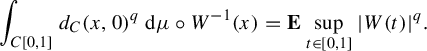 $$ \begin{align*} \int_{C[0,1]} d_C(x,0)^q \, \mathrm{d} \mu\circ W^{-1}(x)=\mathbf{E}\sup_{t\in [0,1]}|W(t)|^q. \end{align*} $$
Hence,
 $$ \begin{align*} \lim_{n \to \infty}\int_{C[0,1]}d_C(x,0)^q \, \mathrm{d} \mu\circ W_n^{-1}(x)=\int_{C[0,1]}d_C(x,0)^q \, \mathrm{d} \mu\circ W^{-1}(x). \end{align*} $$
By taking $\mu _n=\mu \circ W_n^{-1}, \mu =\mu \circ W^{-1}$
and
$\mu _n=\mu \circ W_n^{-1}, \mu =\mu \circ W^{-1}$
and $x_0=0$
in Proposition 2.3 and the fact that
$x_0=0$
in Proposition 2.3 and the fact that $W_n\to _{w} W$
in Lemma 3.1(c), the result follows.
$W_n\to _{w} W$
in Lemma 3.1(c), the result follows.
Theorem 3.4. Let $T:M\rightarrow M$
be a non-uniformly expanding map of order
$T:M\rightarrow M$
be a non-uniformly expanding map of order $p\ge 4$
and suppose that
$p\ge 4$
and suppose that $v:M\rightarrow \mathbb {R}$
is a Hölder observable with
$v:M\rightarrow \mathbb {R}$
is a Hölder observable with $\int _M v \,\mathrm {d}\mu =0$
. Then there exists a constant
$\int _M v \,\mathrm {d}\mu =0$
. Then there exists a constant $C>0$
such that
$C>0$
such that $\mathcal {W}_{{p}/{2}}(W_{n},W)\leq Cn^{-1/4+1/(4(p-1))}$
for all
$\mathcal {W}_{{p}/{2}}(W_{n},W)\leq Cn^{-1/4+1/(4(p-1))}$
for all $n\geq 1$
.
$n\geq 1$
.
We postpone the proof of Theorem 3.4 to §4.
Remark 3.5.
-
(1) Since
$\mathcal {W}_{q}\ \le \mathcal {W}_{p}$
for
$q\le p$
, Theorem 3.4 provides an estimate for
$\mathcal {W}_{q}(W_{n},W)$
for all
$1\le q\le p/2$
,
$p\ge 4$
. -
(2) Our result implies a convergence rate
$O(n^{-1/4+\delta '})$
with respect to the Lévy–Prokhorov distance, where
$\delta '$
depends only on p and
$\delta '$
can be arbitrarily small as
$p\to ~\infty $
. Indeed, for two given probability measures
$\mu $
and
$\nu $
, we have
$\pi (\mu ,\nu )\le \mathcal {W}_{p}(\mu ,\nu )^{{p}/({p+1})}$
; see Proposition 2.6. -
(3) The convergence rate in Theorem 3.4 may not be optimal. However, it is well known that one cannot get a better result than
$O(n^{-1/4})$
by means of the Skorokhod embedding theorem; see [Reference Borovkov6, Reference Sawyer30] for details.


Example 3.6. (Pomeau–Manneville intermittent maps)
A typical example of non-uniformly expanding systems with polynomial tails is the Pomeau–Manneville intermittent map [Reference Liverani, Saussol and Vaienti23, Reference Pomeau and Manneville27]. Consider the map $T:[0,1]\rightarrow [0,1]$
given by
$T:[0,1]\rightarrow [0,1]$
given by
 $$ \begin{align} T(x)= \begin{cases} x(1+2^\gamma x^\gamma) & \text{if } x\in\big[0,\frac{1}{2}\big),\\ 2x-1 & \text{if } x\in\big[\frac{1}{2},1\big], \end{cases} \end{align} $$
where $\gamma \ge 0$
is a parameter. When
$\gamma \ge 0$
is a parameter. When $\gamma =0$
, this is
$\gamma =0$
, this is $Tx=2x $
mod
$Tx=2x $
mod $1$
, which is a uniformly expanding system. It is well known that, for each
$1$
, which is a uniformly expanding system. It is well known that, for each $0\le \gamma <1$
, there is a unique absolutely continuous invariant probability measure
$0\le \gamma <1$
, there is a unique absolutely continuous invariant probability measure $\mu $
. By [Reference Young34], for
$\mu $
. By [Reference Young34], for $0<\gamma <1$
, the map can be modelled by a Young tower with tails
$0<\gamma <1$
, the map can be modelled by a Young tower with tails $O(n^{-{1}/{\gamma }})$
. Further for
$O(n^{-{1}/{\gamma }})$
. Further for $\gamma \in [0,\tfrac 12)$
, the CLT and WIP hold for Hölder continuous observables. We restrict the parameter
$\gamma \in [0,\tfrac 12)$
, the CLT and WIP hold for Hölder continuous observables. We restrict the parameter $\gamma \in (0,\tfrac 12)$
; then the map is a non-uniformly expanding system of order p for any
$\gamma \in (0,\tfrac 12)$
; then the map is a non-uniformly expanding system of order p for any $p<{1}/{\gamma }$
. By Theorem 3.4, we obtain
$p<{1}/{\gamma }$
. By Theorem 3.4, we obtain $\mathcal {W}_{{p}/{2}}(W_{n},W)\leq Cn^{-1/4+\gamma/(4(1-\gamma))+\delta}$
for all
$\mathcal {W}_{{p}/{2}}(W_{n},W)\leq Cn^{-1/4+\gamma/(4(1-\gamma))+\delta}$
for all $\gamma \in (0,\tfrac 14)$
.
$\gamma \in (0,\tfrac 14)$
.
Example 3.7. (Viana maps)
Consider the Viana maps [Reference Viana31] $T_\alpha :S^1\times {\mathbb R}\rightarrow S^1\times {\mathbb R}$
 $$ \begin{align*} T_\alpha(\omega, x)=(l\omega \text{~mod~} 1, a_0+\alpha\sin 2\pi \omega-x^2). \end{align*} $$
Here, $a_0\in (1,2)$
is chosen in such a way that
$a_0\in (1,2)$
is chosen in such a way that $x=0$
is a preperiodic point for the map
$x=0$
is a preperiodic point for the map $g(x)=a_0-x^2$
,
$g(x)=a_0-x^2$
, $\alpha $
is fixed to be sufficiently small and
$\alpha $
is fixed to be sufficiently small and $l\in {\mathbb N}$
with
$l\in {\mathbb N}$
with $l\ge 16$
. The results in [Reference Gouëzel17] show that any T close to the map
$l\ge 16$
. The results in [Reference Gouëzel17] show that any T close to the map $T_\alpha $
in the
$T_\alpha $
in the $C^3$
topology can be modelled by a Young tower with stretched exponential tails, which is a non-uniformly expanding map of order p for all
$C^3$
topology can be modelled by a Young tower with stretched exponential tails, which is a non-uniformly expanding map of order p for all $p\ge 1$
. Hence by Theorem 3.4, for all
$p\ge 1$
. Hence by Theorem 3.4, for all $p\geq 4$
,
$p\geq 4$
, $\mathcal {W}_{{p}/{2}}(W_{n},W)\leq Cn^{-1/4+1/(4(p-1))}$
.
$\mathcal {W}_{{p}/{2}}(W_{n},W)\leq Cn^{-1/4+1/(4(p-1))}$
.
3.2 Non-uniformly hyperbolic diffeomorphism
In this subsection, we introduce the main results for non-uniformly hyperbolic systems in the sense of Young [Reference Young33, Reference Young34]. In this case, we follow the argument in [Reference Korepanov, Kosloff and Melbourne21, Reference Melbourne and Nicol24].
Let $T:M \rightarrow M$
be a diffeomorphism (possibly with singularitiesFootnote †) defined on a Riemannian manifold
$T:M \rightarrow M$
be a diffeomorphism (possibly with singularitiesFootnote †) defined on a Riemannian manifold $(M,d)$
. As in [Reference Melbourne and Nicol24], consider a subset
$(M,d)$
. As in [Reference Melbourne and Nicol24], consider a subset $Y\subset M$
which has a hyperbolic product structure: that is, there exist a continuous family of unstable disks
$Y\subset M$
which has a hyperbolic product structure: that is, there exist a continuous family of unstable disks $\{W^u\}$
and a continuous family of stable disks
$\{W^u\}$
and a continuous family of stable disks $\{W^s\}$
such that:
$\{W^s\}$
such that:
-
(1)
$\mathrm {dim} W^s+ \mathrm {dim} W^u=\mathrm {dim} M$
; -
(2) each
$W^u$
-disk is transversal to each
$W^s$
-disk in a single point; and -
(3)
$Y=(\cup W^u)\cap (\cup W^s)$
.


For $x\in Y$
,
$x\in Y$
, $W^s(x)$
denotes the element in
$W^s(x)$
denotes the element in $\{W^s\}$
containing x.
$\{W^s\}$
containing x.
Furthermore, there is a measurable partition $\{Y_j\}$
of Y such that each
$\{Y_j\}$
of Y such that each $Y_j$
is a union of elements in
$Y_j$
is a union of elements in $\{W^s\}$
and a
$\{W^s\}$
and a $W^u$
such that each element of
$W^u$
such that each element of $\{W^s\}$
intersects
$\{W^s\}$
intersects $W^u$
in one point. Defining an integrable return time
$W^u$
in one point. Defining an integrable return time $R:Y\rightarrow \mathbb {Z}^{+}$
that is constant on each partition
$R:Y\rightarrow \mathbb {Z}^{+}$
that is constant on each partition $Y_j$
, we can get the corresponding induced map
$Y_j$
, we can get the corresponding induced map $F=T^{R}:Y\rightarrow Y$
. The separation time
$F=T^{R}:Y\rightarrow Y$
. The separation time $s(x,y)$
is the greatest integer
$s(x,y)$
is the greatest integer $n\ge 0$
such that
$n\ge 0$
such that $F^nx,F^ny$
lie in the same partition element of Y.
$F^nx,F^ny$
lie in the same partition element of Y.
We assume that there exist $C>0$
and
$C>0$
and $\gamma \in (0,1)$
such that:
$\gamma \in (0,1)$
such that:
-
(1)
$F(W^s(x))\subset W^s(Fx)$
for all
$x\in Y$
; -
(2)
$d(T^n(x),T^n(y))\le C \gamma ^n$
for all
$x\in Y$
,
$y\in W^s(x)$
and
$n\ge 0$
; and -
(3)
$d(T^n(x),T^n(y))\le C \gamma ^{s(x,y)}$
for
$x,y\in W^u$
and
$0\le n<R$
.


As for the non-uniformly expanding map, we can define a Young tower. Let ${\Delta :=\{(x,l):x\in Y, l=0,1,\ldots ,R(x)-1\}}$
and define an extension map
${\Delta :=\{(x,l):x\in Y, l=0,1,\ldots ,R(x)-1\}}$
and define an extension map $f:\Delta \rightarrow \Delta $
,
$f:\Delta \rightarrow \Delta $
,
 $$ \begin{align*} f(x,l):= \begin{cases} (x,l+1) & \text{if } l+1<R(x),\\ (Fx,0) & \text{if } l+1=R(x). \end{cases} \end{align*} $$
We have a projection map $\pi _\Delta :\Delta \rightarrow M$
given by
$\pi _\Delta :\Delta \rightarrow M$
given by $\pi _\Delta (x,l):=T^lx$
and it is a semiconjugacy satisfying
$\pi _\Delta (x,l):=T^lx$
and it is a semiconjugacy satisfying $T\circ \pi _\Delta =\pi _\Delta \circ f$
.
$T\circ \pi _\Delta =\pi _\Delta \circ f$
.
Let $\bar {Y}=Y/\thicksim $
, where
$\bar {Y}=Y/\thicksim $
, where $y\thicksim y'$
if
$y\thicksim y'$
if $y'\in W^s(y)$
; denote by
$y'\in W^s(y)$
; denote by $\bar {\pi }:Y\rightarrow \bar {Y}$
the natural projection. We can also obtain a partition
$\bar {\pi }:Y\rightarrow \bar {Y}$
the natural projection. We can also obtain a partition $\{\bar {Y}_j\}$
of
$\{\bar {Y}_j\}$
of $\bar {Y}$
, a well-defined return time
$\bar {Y}$
, a well-defined return time $\bar {R}:\bar {Y}\rightarrow \mathbb {Z}^{+}$
and a corresponding induced map
$\bar {R}:\bar {Y}\rightarrow \mathbb {Z}^{+}$
and a corresponding induced map $\bar {F}:\bar {Y}\rightarrow \bar {Y}$
, as in the case of Y. In addition, we assume that:
$\bar {F}:\bar {Y}\rightarrow \bar {Y}$
, as in the case of Y. In addition, we assume that:
-
(1)
$\bar {F}|_{\bar {Y}_j}=\bar {T}^{\bar {R}(\bar {Y}_j)}:\bar {Y}_j\rightarrow \bar {Y}$
is a bijection for each j; and -
(2)
$\nu _0={d\bar {\rho }}/({d\bar {\rho }\circ \bar {F}})$
satisfies
$|\log \nu _0(y)-\log \nu _0(y')|\le K\gamma ^{s(y,y')} $
, for all
$y,y'\in \bar {Y}_j$
, where
$\bar {\rho }=\bar {\pi }_\ast \rho $
with
$\rho $
being the Riemannian measure.


Let $\bar {f}:\bar {\Delta }\rightarrow \bar {\Delta }$
denote the corresponding extension map. The projection
$\bar {f}:\bar {\Delta }\rightarrow \bar {\Delta }$
denote the corresponding extension map. The projection $\bar {\pi }:Y\rightarrow \bar {Y}$
extends to the projection
$\bar {\pi }:Y\rightarrow \bar {Y}$
extends to the projection $\bar {\pi }:\Delta \rightarrow \bar {\Delta }$
; here we use the same notation
$\bar {\pi }:\Delta \rightarrow \bar {\Delta }$
; here we use the same notation $\bar {\pi }$
, which should not cause confusion. There exist an
$\bar {\pi }$
, which should not cause confusion. There exist an $\bar {f}$
-invariant probability measure
$\bar {f}$
-invariant probability measure $\bar {\mu }$
on
$\bar {\mu }$
on $\bar {\Delta }$
and an f-invariant probability measure
$\bar {\Delta }$
and an f-invariant probability measure $\mu _{\Delta }$
on
$\mu _{\Delta }$
on $\Delta $
, such that
$\Delta $
, such that $\bar {\pi }:\Delta \rightarrow \bar {\Delta }$
and
$\bar {\pi }:\Delta \rightarrow \bar {\Delta }$
and $\pi _\Delta :\Delta \rightarrow M$
are measure preserving.
$\pi _\Delta :\Delta \rightarrow M$
are measure preserving.
Theorem 3.8. Let $T:M\rightarrow M$
be a non-uniformly hyperbolic transformation of order
$T:M\rightarrow M$
be a non-uniformly hyperbolic transformation of order $p> 2$
. Suppose that
$p> 2$
. Suppose that $v:M\rightarrow \mathbb {R}$
is a Hölder observable with
$v:M\rightarrow \mathbb {R}$
is a Hölder observable with $\int _M v \,\mathrm {d}\mu =0$
. Then
$\int _M v \,\mathrm {d}\mu =0$
. Then $\mathcal {W}_{q}(W_{n},W)\to 0$
in
$\mathcal {W}_{q}(W_{n},W)\to 0$
in $C[0,1]$
for all
$C[0,1]$
for all $1\le q< 2(p-1)$
.
$1\le q< 2(p-1)$
.
Proof. By [Reference Korepanov, Kosloff and Melbourne21, Corollary 5.5], $W_n$
has a finite moment of order
$W_n$
has a finite moment of order $2(p-1)$
. The remaining proof is similar to that of Theorem 3.3.
$2(p-1)$
. The remaining proof is similar to that of Theorem 3.3.
Theorem 3.9. Let $T:M\rightarrow M$
be a non-uniformly hyperbolic transformation of order
$T:M\rightarrow M$
be a non-uniformly hyperbolic transformation of order $p\ge 4$
and suppose that
$p\ge 4$
and suppose that $v:M\rightarrow \mathbb {R}$
is a Hölder observable with
$v:M\rightarrow \mathbb {R}$
is a Hölder observable with $\int _M v \,\mathrm {d}\mu =0$
. Then there exists a constant
$\int _M v \,\mathrm {d}\mu =0$
. Then there exists a constant $C>0$
such that
$C>0$
such that $\mathcal {W}_{{p}/{2}}(W_{n},W)\leq Cn^{-1/4+{1}/{(4(p-1))}}$
for all
$\mathcal {W}_{{p}/{2}}(W_{n},W)\leq Cn^{-1/4+{1}/{(4(p-1))}}$
for all $n\geq 1$
.
$n\geq 1$
.
We postpone the proof of Theorem 3.9 to the next section.
Example 3.10. (Non-uniformly expanding/hyperbolic systems with exponential tails)
In this case, the return time $R\in L^p$
for all p. Hence, for all
$R\in L^p$
for all p. Hence, for all $p\geq 4$
,
$p\geq 4$
, $\mathcal {W}_{{p}/{2}}(W_{n},W)\leq Cn^{-1/4+1/(4(p-1))}$
. Specific examples are:
$\mathcal {W}_{{p}/{2}}(W_{n},W)\leq Cn^{-1/4+1/(4(p-1))}$
. Specific examples are:
-
• some partially hyperbolic systems with a mostly contracting direction [Reference Castro7, Reference Dolgopyat12];
-
• unimodal maps and multimodal maps as in [Reference Korepanov, Kosloff and Melbourne20] for a fixed system; and
-
• Hénon-type attractors [Reference Hénon19]. Let
$T_{a,b}:{\mathbb R}^2\rightarrow {\mathbb R}^2$
be defined by
$T_{a,b}(x,y)= (1-ax^2+y, bx)$
for
$a<2$
,
$b>0$
, where b is small enough depending on a. It follows from [Reference Benedicks and Young3, Reference Benedicks and Young4] that T admits an Sinai–Ruelle–Bowen (SRB) measure and T can be modelled by a Young tower with exponential tails.


4 Proof of Theorems 3.4 and 3.9
4.1 Martingale approximation
The martingale approximation method [Reference Gordin14] is one of the main methods for studying statistical limit properties. In [Reference Korepanov, Kosloff and Melbourne21], Korepanov et al obtained a new version of martingale-coboundary decomposition, which is applicable to non-uniformly hyperbolic systems. In this subsection, we recall some required properties in [Reference Korepanov, Kosloff and Melbourne21].
Proposition 4.1. Let $T:M\rightarrow M$
be a non-uniformly expanding map of order
$T:M\rightarrow M$
be a non-uniformly expanding map of order $p\ge 1$
and suppose that
$p\ge 1$
and suppose that $v:M\rightarrow \mathbb {R}$
is a Hölder observable with
$v:M\rightarrow \mathbb {R}$
is a Hölder observable with $\int _M v\,\mathrm{d}\mu =0$
. Then there is an extension
$\int _M v\,\mathrm{d}\mu =0$
. Then there is an extension $f:\Delta \rightarrow \Delta $
of T such that, for any
$f:\Delta \rightarrow \Delta $
of T such that, for any $v\in C^\eta (M)$
, there exist
$v\in C^\eta (M)$
, there exist $m\in L^{p}(\Delta )$
and
$m\in L^{p}(\Delta )$
and $\chi \in L^{p-1}(\Delta )$
with
$\chi \in L^{p-1}(\Delta )$
with
 $$ \begin{align*} v\circ\pi_\Delta=m+\chi\circ f-\chi,\quad \mathbf{E}(m|f^{-1}\mathcal{M})=0. \end{align*} $$
Moreover, there is a constant $C>0$
such that, for all
$C>0$
such that, for all $v\in C^\eta (M)$
,
$v\in C^\eta (M)$
,
 $$ \begin{align*} \|m\|_{L^p}\le C\|v\|_{\eta},\quad \|\chi\|_{L^{p-1}}\le C\|v\|_{\eta} \end{align*} $$
and, for $n\geq 1$
,
$n\geq 1$
,
 $$ \begin{align*} \Big\|\!\max_{0\le j\le n}|\chi\circ f^j-\chi|\Big\|_{L^p}\le C\|v\|_{\eta}n^{1/p}. \end{align*} $$
Proof. The proposition is a summary of Propositions 2.4, 2.5 and 2.7 in [Reference Korepanov, Kosloff and Melbourne21].
Proposition 4.2. Fix $n\ge 1$
. Then
$n\ge 1$
. Then $\{m\circ f^{n-i},f^{-(n-i)}\mathcal {M};1\le i\le n\}$
is a martingale difference sequence.
$\{m\circ f^{n-i},f^{-(n-i)}\mathcal {M};1\le i\le n\}$
is a martingale difference sequence.
Proof. See, for example [Reference Korepanov, Kosloff and Melbourne21, Proposition 2.9].
Proposition 4.3. If $p\geq 2$
, then
$p\geq 2$
, then $\|\!\max _{k\leq n}|\!\sum _{i=1}^{k}m\circ f^{n-i}|\|_{L^{p}}\leq C\|m\|_{L^p}n^{1/2}$
for all
$\|\!\max _{k\leq n}|\!\sum _{i=1}^{k}m\circ f^{n-i}|\|_{L^{p}}\leq C\|m\|_{L^p}n^{1/2}$
for all $n\ge 1$
.
$n\ge 1$
.
Proof. See the proof in [Reference Korepanov, Kosloff and Melbourne21, Corollary 2.10].
4.2 Proof of Theorem 3.4
Define
 $$ \begin{align*} \zeta_{n,j}:=\frac{1}{\sqrt{n}\sigma}m\circ f^{n-j},\quad \mathcal{F}_{n,j}:=f^{-(n-j)}\mathcal{M} \quad\mathrm{for}\ 1\le j\le n. \end{align*} $$
For $1\le l\le n$
, define the conditional variance
$1\le l\le n$
, define the conditional variance
 $$ \begin{align*} V_{n,l}:=\sum_{j=1}^{l}\mathbf{E}(\zeta_{n,j}^2|\mathcal{F}_{n,j-1}). \end{align*} $$
We set $V_{n,0}=0$
.
$V_{n,0}=0$
.
Define the stochastic process $X_n$
with sample paths in
$X_n$
with sample paths in $C[0,1]$
by
$C[0,1]$
by
 $$ \begin{align} X_{n}(t):=\sum_{j=1}^{k}\zeta_{n,j}+\frac{tV_{n,n}-V_{n,k}}{V_{n,k+1}-V_{n,k}}\zeta_{n,k+1} \quad \textrm{if } V_{n,k}\leq tV_{n,n}<V_{n,k+1}. \end{align} $$
Step 1. Estimate of the Wasserstein distance between ${X}_{{n}}$
and
${X}_{{n}}$
and $B$
. Let B be a standard Brownian motion, that is,
$B$
. Let B be a standard Brownian motion, that is, $B=_d1/\sigma W$
.
$B=_d1/\sigma W$
.
Lemma 4.4. Let $p\ge 4$
. Then, for any
$p\ge 4$
. Then, for any $\delta>0$
, there exists a constant
$\delta>0$
, there exists a constant $C>0$
such that
$C>0$
such that $\mathcal {W}_{{p}/{2}}(X_{n},B)\leq C n^{-(1/4-\delta )}$
for all
$\mathcal {W}_{{p}/{2}}(X_{n},B)\leq C n^{-(1/4-\delta )}$
for all $n\geq 1$
.
$n\geq 1$
.
Proof. (1) Fix $n>0$
. It suffices to deal with a single row of the array
$n>0$
. It suffices to deal with a single row of the array $\{\zeta _{n,j},\mathcal {F}_{n,j}, 1\le j\le n\}$
. By the Skorokhod embedding theorem (see Theorem A.1), there exists a probability space (depending on n) supporting a standard Brownian motion, still denoted by B, which should not cause confusion, and a sequence of non-negative random variables
$\{\zeta _{n,j},\mathcal {F}_{n,j}, 1\le j\le n\}$
. By the Skorokhod embedding theorem (see Theorem A.1), there exists a probability space (depending on n) supporting a standard Brownian motion, still denoted by B, which should not cause confusion, and a sequence of non-negative random variables $\tau _1,\ldots , \tau _n$
such that, for
$\tau _1,\ldots , \tau _n$
such that, for $T_i=\sum _{j=1}^{i}\tau _j$
, we have
$T_i=\sum _{j=1}^{i}\tau _j$
, we have $\sum _{j=1}^{i}\zeta _{n,j}=B(T_i)$
with
$\sum _{j=1}^{i}\zeta _{n,j}=B(T_i)$
with $1\le i\le n$
. In particular, we set
$1\le i\le n$
. In particular, we set $T_{0}=0$
. Then, on this probability space and for this Brownian motion, we aim to show that, for any
$T_{0}=0$
. Then, on this probability space and for this Brownian motion, we aim to show that, for any $\delta>0$
, there exists a constant
$\delta>0$
, there exists a constant $C>0$
such that
$C>0$
such that
 $$ \begin{align*} \Big\|\!\sup_{t\in[0,1]}|X_{n}(t)-B(t)|\Big\|_{L^{{p}/{2}}}\leq Cn^{-({1}/{4}-\delta)} \quad \mathrm{for~all~}n\ge1. \end{align*} $$
Thus, the result follows from Definition 2.1.
For ease of exposition when there is no ambiguity, we will write $\zeta _j$
and
$\zeta _j$
and $V_k$
instead of
$V_k$
instead of $\zeta _{n,j}$
and
$\zeta _{n,j}$
and $V_{n,k}$
, respectively. Then, by (4.1),
$V_{n,k}$
, respectively. Then, by (4.1),
 $$ \begin{align} X_{n}(t)=B(T_{k})+\bigg(\frac{tV_{n}-V_{k}}{V_{k+1}-V_{k}}\bigg)(B(T_{k+1})-B(T_{k}))\quad \mathrm{if}\ V_{k}\leq tV_{n}<V_{k+1}. \end{align} $$
(2) Note that Theorem A.1(3) implies that
 $$ \begin{align*} T_k-V_k=\sum_{i=1}^{k}(\tau_{i}-\mathbf{E}(\tau_{i}|\mathcal{B}_{i-1})) \quad \mathrm{if}\ 1\le k\le n, \end{align*} $$
where $\mathcal {B}_{i}$
is the
$\mathcal {B}_{i}$
is the $\sigma $
-field generated by all events up to
$\sigma $
-field generated by all events up to $T_i$
for
$T_i$
for $1\le i\le n$
. Therefore,
$1\le i\le n$
. Therefore, $\{T_k-V_k, \mathcal {B}_{k}, 1\le k\le n\}$
is a martingale. By the Burkholder inequality and the conditional Jensen inequality, for all
$\{T_k-V_k, \mathcal {B}_{k}, 1\le k\le n\}$
is a martingale. By the Burkholder inequality and the conditional Jensen inequality, for all $p\ge 4$
,
$p\ge 4$
,
 $$ \begin{align*} \Big\|\!\max_{1\le k\le n}|T_k-V_{k}|\Big\|_{L^{{p}/{2}}} &\le Cn^{{1}/{2}} \max_{1\le k\le n}\|\tau_{k}-\mathbf{E}(\tau_{k}|\mathcal{B}_{k-1})\|_{L^{{p}/{2}}}\\ &\le Cn^{{1}/{2}} \max_{1\le k\le n}\|\tau_{k}\|_{L^{{p}/{2}}}. \end{align*} $$
It follows from Theorem A.1(4) that $\mathbf {E}(\tau _{k}^{p/2})\le 2\Gamma ( {p}/{2}+1)\mathbf {E}(\zeta _{k}^{p})$
for each k. So
$\mathbf {E}(\tau _{k}^{p/2})\le 2\Gamma ( {p}/{2}+1)\mathbf {E}(\zeta _{k}^{p})$
for each k. So
 $$ \begin{align} \Big\|\!\max_{1\le k\le n}|T_k-V_{k}|\Big\|_{L^{{p}/{2}}} \le Cn^{{1}/{2}} \max_{1\le k\le n}\|\zeta_{k}\|_{L^p}^2= Cn^{-{1}/{2}}\|m\|_{L^p}^{2}. \end{align} $$
On the other hand, it follows from [Reference Antoniou and Melbourne2, Proposition 4.1] that
 $$ \begin{align} \|V_{n}-1\|_{L^{{p}/{2}}}\le C n^{-{1}/{2}}\|v\|_{\eta}^{2}. \end{align} $$
(3) Based on the above estimates, by Chebyshev’s inequality,
 $$ \begin{align} \begin{aligned} \mu(|T_{n}-1|>1)&\le \mathbf{E}|T_{n}-1|^{{p}/{2}} \le 2^{p/2-1}\{\mathbf{E}|T_{n}-V_{n}|^{{p}/{2}}+\mathbf{E}|V_{n}-1|^{{p}/{2}}\}\\ &\le Cn^{-{p}/{4}}(\|m\|_{L^p}^{p}+\|v\|_{\eta}^{p}).\\ \end{aligned} \end{align} $$
According to the Hölder inequality, (4.5) and Proposition 4.3, we deduce that
 $$ \begin{align*} I:&=\Big\| 1_{\{|T_{n}-1|>1\}}\sup_{t\in[0,1]}|X_{n}(t)-B(t)|\Big\|_{L^{{p}/{2}}}\\ &\le (\mu(|T_{n}-1|>1))^{1/p}\Big\| \sup_{t\in[0,1]}|X_{n}(t)-B(t)|\Big\|_{L^{p}}\\ &\le (\mu(|T_{n}-1|>1))^{1/p}\Big(\Big\|\!\sup_{t\in[0,1]}|X_{n}(t)|\Big\|_{L^{p}}+\Big\|\!\sup_{t\in[0,1]}|B(t)|\Big\|_{L^{p}}\Big)\\ &\le Cn^{-{1}/{4}}. \end{align*} $$
(4) We now estimate $|X_{n}-B|$
on the set
$|X_{n}-B|$
on the set $\{|T_{n}-1|\le 1\}$
: that is,
$\{|T_{n}-1|\le 1\}$
: that is,
 $$ \begin{align*} &\Big\| 1_{\{|T_{n}-1|\le 1\}}\sup_{t\in[0,1]}|X_{n}(t)-B(t)|\Big\|_{L^{{p}/{2}}}\\ &\quad\le \Big\| 1_{\{|T_{n}-1|\le 1\}}\sup_{t\in[0,1]}|X_{n}(t)-B(T_{k})|\Big\|_{L^{p/2}}+\Big\|1_{\{|T_{n}-1|\le 1\}}\sup_{t\in[0,1]}|B(T_{k})-B(t)|\Big\|_{L^{{p}/{2}}}\\ &\quad =: I_1 + I_2. \end{align*} $$
For $I_1$
, it follows from (4.2) that
$I_1$
, it follows from (4.2) that
 $$ \begin{align*} \sup_{t\in[0,1]}|X_{n}(t)-B(T_{k})|\le \max_{0\le k\le n-1}|B(T_{k+1})-B(T_{k})|=\max_{0\le k\le n-1}|\zeta_{k+1}|. \end{align*} $$
By Proposition A.2,
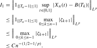 $$ \begin{align*} I_1&=\Big\| 1_{\{|T_{n}-1|\le 1\}}\sup_{t\in[0,1]}|X_{n}(t)-B(T_{k})|\Big\|_{L^{p}}\nonumber\\ &\le \Big\| 1_{\{|T_{n}-1|\le 1\}}\max_{0\le k\le n-1}|\zeta_{k+1}|\Big\|_{L^{p}}\nonumber\\ &\le \Big\| \max_{0\le k\le n-1}|\zeta_{k+1}|\Big\|_{L^{p}}\nonumber\\ &\le Cn^{-({1}/{2}-{1}/{p})}. \end{align*} $$
(5) We now consider $I_{2}$
on the set
$I_{2}$
on the set $\{|T_{n}-1|\le 1\}$
. Take
$\{|T_{n}-1|\le 1\}$
. Take $p_1>p$
. Then it is well known that
$p_1>p$
. Then it is well known that
 $$ \begin{align} \mathbf{E}|B(t)-B(s)|^{p_1}\le c|t-s|^{{p_1}/{2}} \quad \text{for all~} s,t\in [0,2]. \end{align} $$
So, it follows from Kolmogorov’s continuity theorem that, for each $0<\gamma <1/2-{1}/ ({p_1})$
, the process
$0<\gamma <1/2-{1}/ ({p_1})$
, the process $B(\cdot )$
admits a version, still denoted by B, such that, for almost all
$B(\cdot )$
admits a version, still denoted by B, such that, for almost all $\omega $
, the sample path
$\omega $
, the sample path $t\mapsto B(t,\omega )$
is Hölder continuous with exponent
$t\mapsto B(t,\omega )$
is Hölder continuous with exponent $\gamma $
and
$\gamma $
and
 $$ \begin{align*} \Big\|\!\sup_{s,t\in[0,2]\atop s\neq t}\frac{|B(s)-B(t)|}{|s-t|^{\gamma}}\Big\|_{L^{p_1}}< \infty. \end{align*} $$
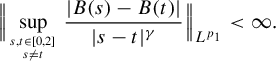
In particular,
 $$ \begin{align} \Big\|\!\sup_{s,t\in[0,2]\atop s\neq t}\frac{|B(s)-B(t)|}{|s-t|^{\gamma}}\Big\|_{L^{p}}< \infty. \end{align} $$
As for $|T_{k}-t|$
,
$|T_{k}-t|$
,
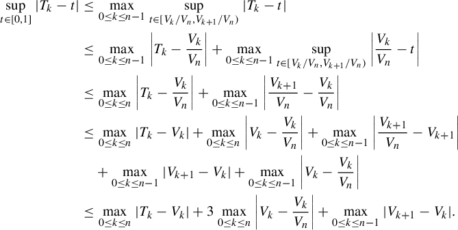 $$ \begin{align*} \sup_{t\in[0,1]}|T_{k}-t|&\le \max_{0\le k\le n-1}\sup_{t\in[{V_{k}}/{V_{n}},{V_{k+1}}/{V_{n}})}|T_{k}-t|\\ &\le \max_{0\le k\le n-1}\bigg|T_{k}-\frac{V_{k}}{V_{n}}\bigg|+\max_{0\le k\le n-1}\sup_{t\in[{V_{k}}/{V_{n}},{V_{k+1}}/{V_{n}})}\bigg|\frac{V_{k}}{V_{n}}-t\bigg|\\ &\le \max_{0\le k\le n}\bigg|T_{k}-\frac{V_{k}}{V_{n}}\bigg|+\max_{0\le k\le n-1}\bigg|\frac{V_{k+1}}{V_{n}}-\frac{V_{k}}{V_{n}}\bigg|\\ &\le \max_{0\le k\le n}|T_{k}-V_{k}|+\max_{0\le k\le n}\bigg|V_{k}-\frac{V_{k}}{V_{n}}\bigg|+\max_{0\le k\le n-1}\bigg|\frac{V_{k+1}}{V_{n}}-V_{k+1}\bigg|\\ &\quad +\max_{0\le k\le n-1}|V_{k+1}-V_{k}|+\max_{0\le k\le n-1}\bigg|V_{k}-\frac{V_{k}}{V_{n}}\bigg|\\ &\le \max_{0\le k\le n}|T_{k}-V_{k}| + 3\max_{0\le k\le n}\bigg|V_{k}-\frac{V_{k}}{V_{n}}\bigg| +\max_{0\le k\le n-1}|V_{k+1}-V_{k}|. \end{align*} $$
Note that $T_{0}=V_{0}=0$
and
$T_{0}=V_{0}=0$
and $\gamma \le 1$
, so
$\gamma \le 1$
, so
 $$ \begin{align*} \sup_{t\in[0,1]}|T_{k}-t|^{\gamma}\le \max_{1\le k\le n}|T_{k}-V_{k}|^{\gamma} + 3^\gamma\max_{1\le k\le n}\bigg|V_{k}-\frac{V_{k}}{V_{n}}\bigg|^{\gamma} +\max_{0\le k\le n-1}|V_{k+1}-V_{k}|^{\gamma}. \end{align*} $$
Hence,
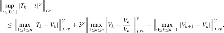 $$ \begin{align} &\Big\|\!\sup_{t\in[0,1]}|T_{k}-t|^{\gamma}\Big\|_{L^{p}}\nonumber\\ &\quad\le \Big\|\!\max_{1\le k\le n}|T_{k}-V_{k}|\Big\|_{L^{\gamma p}}^{\gamma} +3^\gamma \bigg\|\!\max_{1\le k\le n}\bigg|V_{k}-\frac{V_{k}}{V_{n}}\bigg|\bigg\|_ {L^{\gamma p}}^{\gamma} +\Big\|\!\max_{0\le k\le n-1}|V_{k+1}-V_{k}|\Big\|_ {L^{\gamma p}}^{\gamma}. \end{align} $$
For the first term, since $\gamma < \tfrac 12$
, it follows from (4.3) that
$\gamma < \tfrac 12$
, it follows from (4.3) that
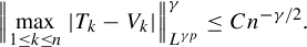 $$ \begin{align} \Big\|\!\max_{1\le k\le n}|T_{k}-V_{k}|\Big\|_{L^{\gamma p}}^{\gamma}\le Cn^{-{\gamma}/{2}}. \end{align} $$
For the second term, since $|V_{k}-{V_{k}}/{V_{n}}|=V_k|1-1/{V_n}|$
,
$|V_{k}-{V_{k}}/{V_{n}}|=V_k|1-1/{V_n}|$
,
 $$ \begin{align*}\max_{1\le k\le n}\bigg|V_{k}-\frac{V_{k}}{V_{n}}\bigg|=V_n \bigg|1-\frac1{V_n}\bigg|=|V_{n}-1|.\end{align*} $$
Hence, by (4.4),
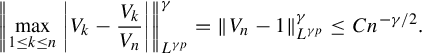 $$ \begin{align} \bigg\|\!\max_{1\le k\le n}\bigg|V_{k}-\frac{V_{k}}{V_{n}}\bigg|\bigg\|_ {L^{\gamma p}}^{\gamma} =\|V_{n}-1\|_{L^{\gamma p}}^{\gamma}\le Cn^{-{\gamma}/{2}}. \end{align} $$
As for the last term, note that $|V_{k}-V_{k-1}|=\mathbf {E}(\zeta _{k}^2|\mathcal {F}_{k-1}) =\mathbf {E}(({1}/{n\sigma ^2})m^2|f^{-1}\mathcal {M})\circ f^{n-k}$
for all
$|V_{k}-V_{k-1}|=\mathbf {E}(\zeta _{k}^2|\mathcal {F}_{k-1}) =\mathbf {E}(({1}/{n\sigma ^2})m^2|f^{-1}\mathcal {M})\circ f^{n-k}$
for all $1\le k\le n$
. So,
$1\le k\le n$
. So,
 $$ \begin{align} \Big\|\!\max_{0\le k\le n-1}|V_{k+1}-V_{k}|\Big\|_ {L^{\gamma p}}^{\gamma}=\bigg\|\!\max_{1\le k\le n}\bigg|\mathbf{E}\bigg(\frac{m^2}{n\sigma^2}|f^{-1}\mathcal{M}\bigg)\circ f^{n-k}\bigg|\bigg\|_{L^{\gamma p}}^{\gamma} \le Cn^{-(\gamma-{2\gamma}/{p})}, \end{align} $$
where the inequality follows from Proposition A.2.
Based on the above estimates (4.9)–(4.11),
 $$ \begin{align} \Big\|\!\sup_{t\in[0,1]}|T_{k}-t|^{\gamma}\Big\|_{L^{p}} \le C(n^{-{\gamma}/{2}}+n^{-(\gamma-{2\gamma}/{p})}) \le C n^{-{\gamma}/{2}}, \end{align} $$
where the last inequality holds since $\gamma < \tfrac 12$
,
$\gamma < \tfrac 12$
, $1-{2}/{p}\ge \tfrac 12$
.
$1-{2}/{p}\ge \tfrac 12$
.
On the set $\{|T_{n}-1|\le 1\}$
, note that
$\{|T_{n}-1|\le 1\}$
, note that
 $$ \begin{align*} \sup_{t\in[0,1]}|B(T_{k})-B(t)|\le \bigg[\,\sup_{s,t\in[0,2]\atop s\neq t}\frac{|B(s)-B(t)|}{|s-t|^{\gamma}}\bigg]\Big[\sup_{t\in[0,1]}|T_{k}-t|^{\gamma}\Big]. \end{align*} $$
Since $0<\gamma <\tfrac 12-{1}/({p_1})$
, by the Hölder inequality, (4.7) and (4.12),
$0<\gamma <\tfrac 12-{1}/({p_1})$
, by the Hölder inequality, (4.7) and (4.12),
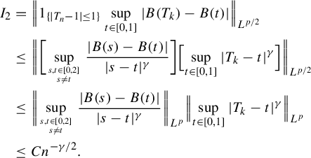 $$ \begin{align*} I_2&=\Big\|1_{\{|T_{n}-1|\le 1\}}\sup_{t\in[0,1]}|B(T_{k})-B(t)|\Big\|_{L^{{p}/{2}}}\\ &\le \bigg\|\bigg[\!\sup_{s,t\in[0,2]\atop s\neq t}\frac{|B(s)-B(t)|}{|s-t|^{\gamma}}\bigg]\Big[\!\sup_{t\in[0,1]}|T_{k}-t|^{\gamma}\Big]\bigg\|_{L^{{p}/{2}}}\\ &\le \bigg\|\!\sup_{s,t\in[0,2]\atop s\neq t}\frac{|B(s)-B(t)|}{|s-t|^{\gamma}}\bigg\|_{L^{p}}\Big\|\!\sup_{t\in[0,1]}|T_{k}-t|^{\gamma}\Big\|_{L^{p}}\\ &\le C n^{-{\gamma}/{2}}. \end{align*} $$
Note that $p_1$
can be taken arbitrarily large in (4.6), which implies that
$p_1$
can be taken arbitrarily large in (4.6), which implies that $\gamma $
can be chosen sufficiently close to
$\gamma $
can be chosen sufficiently close to $\tfrac 12$
. So, for any
$\tfrac 12$
. So, for any $\delta>0$
, we can choose
$\delta>0$
, we can choose $p_1$
large enough such that
$p_1$
large enough such that $I_2\le Cn^{-1/4+\delta }$
. The result now follows from the above estimates for
$I_2\le Cn^{-1/4+\delta }$
. The result now follows from the above estimates for $I,I_1$
and
$I,I_1$
and $I_2$
.
$I_2$
.
Step 2. Estimate of the convergence rate between ${W}_{{n}}$
and
${W}_{{n}}$
and ${X}_{{n}}$
. The proof is almost identical to that in [Reference Antoniou and Melbourne2, §4.1], so we only sketch it here.
${X}_{{n}}$
. The proof is almost identical to that in [Reference Antoniou and Melbourne2, §4.1], so we only sketch it here.
Proposition 4.5. [Reference Antoniou and Melbourne2, Proposition 4.6]
For $n\ge 1$
, define
$n\ge 1$
, define
 $$ \begin{align*} Z_n:=\max_{0\le i,l\le\sqrt{n}}\bigg|\!\sum_{j=i\sqrt{n}}^{i\sqrt{n}+l-1} v\circ T^j\bigg|. \end{align*} $$
Then:
-
(a)
$|\!\sum _{j=a}^{b-1}v\circ T^j|\le Z_n((b-a)(n^{1/2}-1)^{-1}+3)$
for all
$0\le a<b \le n$
; and -
(b)
$\|Z_n\|_{L^{2(p-1)}}\le C\|v\|_{\eta }n^{1/4+1/(4(p-1))}$
for all
$n\ge 1$
.


Define a continuous transformation $g:C[0,1]\rightarrow C[0,1]$
by
$g:C[0,1]\rightarrow C[0,1]$
by $g(u)(t):= u(1)- u (1-t)$
.
$g(u)(t):= u(1)- u (1-t)$
.
Lemma 4.6. Let $p>2$
. Then there exists a constant
$p>2$
. Then there exists a constant $C>0$
such that
$C>0$
such that $\mathcal {W}_{p-1}(g\circ W_{n}\circ \pi _\Delta ,\sigma X_{n})\leq Cn^{-1/4+{1}/({4(p-1)})}$
for all
$\mathcal {W}_{p-1}(g\circ W_{n}\circ \pi _\Delta ,\sigma X_{n})\leq Cn^{-1/4+{1}/({4(p-1)})}$
for all $n\geq 1$
, recalling that
$n\geq 1$
, recalling that $\pi _\Delta :\Delta \to M$
is the projection map.
$\pi _\Delta :\Delta \to M$
is the projection map.
Proof. Since $\mathcal {W}_{p-1}(g\circ W_{n}\circ \pi _\Delta ,\sigma X_{n})\le \|\!\sup _{t\in [0,1]}|g\circ W_{n}(t)\circ \pi _\Delta -\sigma X_n(t)|\|_{L^{p-1}}$
, following the proof of [Reference Antoniou and Melbourne2, Lemma 4.7], we can obtain the conclusion.
$\mathcal {W}_{p-1}(g\circ W_{n}\circ \pi _\Delta ,\sigma X_{n})\le \|\!\sup _{t\in [0,1]}|g\circ W_{n}(t)\circ \pi _\Delta -\sigma X_n(t)|\|_{L^{p-1}}$
, following the proof of [Reference Antoniou and Melbourne2, Lemma 4.7], we can obtain the conclusion.
Proof of Theorem 3.4
Note that $g\circ g= \mathrm {Id}$
and g is Lipschitz with
$g\circ g= \mathrm {Id}$
and g is Lipschitz with $\mathrm {Lip}g \le 2$
. It follows from Proposition 2.4 that
$\mathrm {Lip}g \le 2$
. It follows from Proposition 2.4 that
 $$ \begin{align*} \mathcal{W}_{{p}/{2}}(W_{n},W)= \mathcal{W}_{{p}/{2}}(g(g\circ W_{n}),g(g\circ W))\le 2\mathcal{W}_{{p}/{2}}(g\circ W_{n},g\circ W). \end{align*} $$
Since $\pi _\Delta $
is a semiconjugacy,
$\pi _\Delta $
is a semiconjugacy, $W_n \circ \pi _\Delta =_d W_n$
. Also,
$W_n \circ \pi _\Delta =_d W_n$
. Also, $g(W)=_d W=_d\sigma B$
. By Lemmas 4.4 and 4.6, for
$g(W)=_d W=_d\sigma B$
. By Lemmas 4.4 and 4.6, for $p\ge 4$
,
$p\ge 4$
,
 $$ \begin{align*} \mathcal{W}_{{p}/{2}}(g\circ W_{n},g\circ W)&=\mathcal{W}_{{p}/{2}}(g\circ W_{n}\circ \pi_\Delta ,W)\\&\le \mathcal{W}_{{p}/{2}}(g\circ W_{n}\circ \pi_\Delta ,\sigma X_n)+\mathcal{W}_{{p}/{2}}(\sigma X_n ,\sigma B)\\&\le Cn^{-1/4+1/(4(p-1))}+Cn^{-1/4+\delta}\le Cn^{-1/4+1/(4(p-1))}, \end{align*} $$
where the last inequality holds because $\delta>0$
can be taken arbitrarily small.
$\delta>0$
can be taken arbitrarily small.
4.3 Proof of Theorem 3.9
The proof is based on the following Lemma 4.7 which is presented in detail in [Reference Korepanov, Kosloff and Melbourne21, §5].
Lemma 4.7. Let $p\ge 1$
,
$p\ge 1$
, $\eta \in (0,1]$
. Suppose that
$\eta \in (0,1]$
. Suppose that $T:M\rightarrow M$
is a non-uniformly hyperbolic transformation with the return time
$T:M\rightarrow M$
is a non-uniformly hyperbolic transformation with the return time $R\in L^p$
and that
$R\in L^p$
and that $v:M\rightarrow \mathbb {R}$
is a Hölder observable. Then:
$v:M\rightarrow \mathbb {R}$
is a Hölder observable. Then:
-
(1)
$\bar {f}:\bar {\Delta }\rightarrow \bar {\Delta }$
is a non-uniformly expanding map of order p; and -
(2) there exists
$\theta \in (0,1)$
such that, for all
$v\in C^\eta (M)$
, there exist
$\phi \in C^\theta (\bar {\Delta })$
and
${\psi \in L^\infty (\Delta )}$
such that
$v\circ \pi _\Delta =\phi \circ \bar {\pi }+\psi -\psi \circ f$
. Moreover,
$|\psi |_\infty \le C\|v\|_\eta $
,
$\|\phi \|_\theta \le C\|v\|_\eta $
.


Proof of Theorem 3.9
As the definition of $W_n$
in (3.1), define
$W_n$
in (3.1), define $\overline {W}_n(t)\kern1.2pt{:=}\kern1.2pt({1}/{\sqrt {n}})\sum _{j=0}^{nt-1}\phi \kern1.2pt{\circ} \bar {f}^j$
for
$\overline {W}_n(t)\kern1.2pt{:=}\kern1.2pt({1}/{\sqrt {n}})\sum _{j=0}^{nt-1}\phi \kern1.2pt{\circ} \bar {f}^j$
for $t={j}/{n}, 1\le j\le n$
, and linearly interpolate to obtain the process
$t={j}/{n}, 1\le j\le n$
, and linearly interpolate to obtain the process ${\overline {W}_n\in C[0,1]}$
, where
${\overline {W}_n\in C[0,1]}$
, where $\phi $
is from Lemma 4.7. By Lemma 4.7, we have
$\phi $
is from Lemma 4.7. By Lemma 4.7, we have $|\overline {W}_n(t)\circ \bar {\pi }-W_n\circ \pi _\Delta |_\infty \le Cn^{-1/2}|\psi |_\infty $
by simple computations. Since
$|\overline {W}_n(t)\circ \bar {\pi }-W_n\circ \pi _\Delta |_\infty \le Cn^{-1/2}|\psi |_\infty $
by simple computations. Since $\bar {\pi }, \pi _\Delta $
are semiconjugacies,
$\bar {\pi }, \pi _\Delta $
are semiconjugacies, $\mathcal {W}_{{p}/{2}}(\overline {W}_n,\kern-0.5pt W_{n})\kern1pt{=}\mathcal {W}_{{p}/{2}}(\overline {W}_n\circ \bar {\pi },W_n\circ \pi _\Delta )\le Cn^{-1/2}$
. It follows from Lemma 4.7 that
$\mathcal {W}_{{p}/{2}}(\overline {W}_n,\kern-0.5pt W_{n})\kern1pt{=}\mathcal {W}_{{p}/{2}}(\overline {W}_n\circ \bar {\pi },W_n\circ \pi _\Delta )\le Cn^{-1/2}$
. It follows from Lemma 4.7 that $\bar {f}$
is a non-uniformly expanding map of order p and that
$\bar {f}$
is a non-uniformly expanding map of order p and that $\phi $
is a Hölder continuous observable with
$\phi $
is a Hölder continuous observable with $\int _{\bar {\Delta }} \phi \, \mathrm {d}\bar {\mu }=0$
. By Theorem 3.4, for
$\int _{\bar {\Delta }} \phi \, \mathrm {d}\bar {\mu }=0$
. By Theorem 3.4, for $p\ge 4$
,
$p\ge 4$
, $\mathcal {W}_{{p}/{2}}(\overline {W}_{n},W)\le Cn^{-1/4+1/(4(p-1))}$
. Hence,
$\mathcal {W}_{{p}/{2}}(\overline {W}_{n},W)\le Cn^{-1/4+1/(4(p-1))}$
. Hence, $\mathcal {W}_{{p}/{2}}(W_{n},W)\le \mathcal {W}_{{p}/{2}}(W_{n},\overline {W}_n)+ \mathcal {W}_{{p}/{2}}(\overline {W}_{n},W)\le Cn^{-1/4+1/(4(p-1))}$
.
$\mathcal {W}_{{p}/{2}}(W_{n},W)\le \mathcal {W}_{{p}/{2}}(W_{n},\overline {W}_n)+ \mathcal {W}_{{p}/{2}}(\overline {W}_{n},W)\le Cn^{-1/4+1/(4(p-1))}$
.
5 Application to homogenization problem
We consider fast–slow systems of the discrete form
 $$ \begin{align} x_\epsilon(n+1)=x_\epsilon(n)+\epsilon^2g(x_\epsilon(n),y(n),\epsilon)+\epsilon h(x_\epsilon(n))v(y(n)),\quad ~x_\epsilon(0)=\xi, \end{align} $$
where $g:\mathbb {R}\times M\times {\mathbb R}^+\rightarrow \mathbb {R}$
,
$g:\mathbb {R}\times M\times {\mathbb R}^+\rightarrow \mathbb {R}$
, $h:\mathbb {R}\rightarrow \mathbb {R}$
satisfy some regularity conditions and
$h:\mathbb {R}\rightarrow \mathbb {R}$
satisfy some regularity conditions and ${v\in C^\eta (M)}$
with
${v\in C^\eta (M)}$
with $\int _M v \,\mathrm {d}\mu =0$
. The fast variables
$\int _M v \,\mathrm {d}\mu =0$
. The fast variables $y(n)\in M$
are generated by iterating a non-uniformly expanding map: that is
$y(n)\in M$
are generated by iterating a non-uniformly expanding map: that is $y(n+1)=Ty(n)$
,
$y(n+1)=Ty(n)$
, $y(0)=y_0$
. Here,
$y(0)=y_0$
. Here, $T:M\to M$
satisfies the setting in §3.1 The initial condition
$T:M\to M$
satisfies the setting in §3.1 The initial condition $\xi \in {\mathbb R}$
is fixed and
$\xi \in {\mathbb R}$
is fixed and $y_0\in M$
is chosen randomly, which is the reason for the emergence of randomness from deterministic dynamical systems.
$y_0\in M$
is chosen randomly, which is the reason for the emergence of randomness from deterministic dynamical systems.
We have the following regularity conditions.
-
(1)
$ g:\mathbb {R}\times M\times {\mathbb R}^+\rightarrow \mathbb {R}$
is bounded. -
(2)
$ g(x,y,0)$
is Lipschitz in x uniformly in y with Lipchitz constant L; that is,
$|g(x_1,y,0)-g(x_2,y,0)|\le L|x_1-x_2|$
for all
$x_1,x_2\in \mathbb {R}, y\in M$
. -
(3)
$\sup _{x\in {\mathbb R}}\sup _{y\in M}|g(x,y,\epsilon )-g(x,y,0)|\le C\epsilon ^{1/3}$
. -
(4)
$ g(x,y,0)$
is Hölder continuous in y uniformly in x: that is,
$\sup _{x\in {\mathbb R}}|g(x,\cdot ,0)|_\eta <\infty $
. -
(5) h is exact; that is,
$h={1}/{\psi '}$
, where
$\psi $
is a monotone differentiable function and
$\psi '$
denotes the derived function. Moreover,
$h, h',h", {1}/{h}$
are bounded.


Let ${\hat x}_\epsilon (t)=x_\epsilon (t\epsilon ^{-2})$
for
${\hat x}_\epsilon (t)=x_\epsilon (t\epsilon ^{-2})$
for $t=0, \epsilon ^2, 2\epsilon ^2,\ldots, $
and linearly interpolate to obtain
$t=0, \epsilon ^2, 2\epsilon ^2,\ldots, $
and linearly interpolate to obtain ${\hat x}_\epsilon \in C[0,1]$
. Then it follows from [Reference Gottwald and Melbourne15, Theorem 1.3] that
${\hat x}_\epsilon \in C[0,1]$
. Then it follows from [Reference Gottwald and Melbourne15, Theorem 1.3] that ${\hat x}_\epsilon \rightarrow _{w} X$
in
${\hat x}_\epsilon \rightarrow _{w} X$
in $C[0,1]$
, where X is the solution to the Stratonovich stochastic differential equation (SDE)
$C[0,1]$
, where X is the solution to the Stratonovich stochastic differential equation (SDE)
 $$ \begin{align} \mathrm{d}X=\bigg\{ \bar{g}(X)-\frac{1}{2}h(X)h'(X)\int_{M}v^{2}\,\mathrm{d}\mu\bigg\}\mathrm{d}t+h(X)\circ \mathrm{d}W,\quad ~X(0)=\xi. \end{align} $$
Here, W is a Brownian motion with mean zero and variance $\sigma ^2$
and
$\sigma ^2$
and $\bar {g}(x)=\int _{M}g(x,y,0)\,\mathrm {d}\mu (y)$
.
$\bar {g}(x)=\int _{M}g(x,y,0)\,\mathrm {d}\mu (y)$
.
Define $W_\epsilon (t)=\epsilon \sum _{j=0}^{t\epsilon ^{-2}-1}v(y(j))$
for
$W_\epsilon (t)=\epsilon \sum _{j=0}^{t\epsilon ^{-2}-1}v(y(j))$
for $t=0, \epsilon ^2, 2\epsilon ^2,\ldots ,$
and linearly interpolate to obtain
$t=0, \epsilon ^2, 2\epsilon ^2,\ldots ,$
and linearly interpolate to obtain $W_\epsilon \in C[0,1]$
. Comparing
$W_\epsilon \in C[0,1]$
. Comparing $W_\epsilon $
with
$W_\epsilon $
with $W_n$
, we can see that
$W_n$
, we can see that $\epsilon $
is identified with
$\epsilon $
is identified with $n^{-1/2}$
. Hence, it follows from Theorem 3.4 that
$n^{-1/2}$
. Hence, it follows from Theorem 3.4 that $\mathcal {W}_{{p}/{2}}(W_\epsilon ,W)=O(\epsilon ^{({p-2})/{2(p-1)}})$
.
$\mathcal {W}_{{p}/{2}}(W_\epsilon ,W)=O(\epsilon ^{({p-2})/{2(p-1)}})$
.
Theorem 5.1. Let $T:M\rightarrow M$
be a non-uniformly expanding map of order
$T:M\rightarrow M$
be a non-uniformly expanding map of order $p\ge 4$
. Suppose that the regularity conditions hold. Then there exists a constant
$p\ge 4$
. Suppose that the regularity conditions hold. Then there exists a constant $C>0$
such that
$C>0$
such that
 $$ \begin{align*} \mathcal{W}_{{p}/{2}}({\hat x}_\epsilon, X)\le \begin{cases} C\epsilon^{({p-2})/{2p}}\quad & \text{if }4\le p\le 6,\\ C\epsilon^{{1}/{3}}(-\log\epsilon)^{{1}/{4}}\quad & \text{if }p>6. \end{cases} \end{align*} $$
Proof. The proof follows from the argument in [Reference Antoniou and Melbourne2]. First, suppose that $h(x)\equiv 1$
and let
$h(x)\equiv 1$
and let $N=[\epsilon ^{-4/3}]$
. By [Reference Antoniou and Melbourne2, Proposition 5.4], we can write
$N=[\epsilon ^{-4/3}]$
. By [Reference Antoniou and Melbourne2, Proposition 5.4], we can write
 $$ \begin{align*} {\hat x}_\epsilon(t)=\xi+W_\epsilon(t)+D_\epsilon(t)+E_\epsilon(t)+\int_{0}^{t}\bar{g}({\hat x}_\epsilon(s))\,\mathrm{d} s, \end{align*} $$
where
 $$ \begin{align*} &D_\epsilon(t)=\epsilon^{{2}/{3}}\sum_{n=0}^{[t\epsilon^{-{2}/{3}}]-1}J_{\epsilon}(n), \quad J_\epsilon(n)=\epsilon^{{4}/{3}}\sum_{j=nN}^{(n+1)N-1}\tilde {g}(x_\epsilon(nN),y(j)),\\ &\qquad\qquad\quad\qquad\qquad \tilde {g}(x,y)=g(x,y,0)-\bar g(x) \end{align*} $$
and
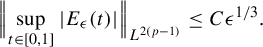 $$ \begin{align} \Big\|\!\sup_{t\in[0,1]}|E_\epsilon(t)|\Big\|_{L^{2(p-1)}}\le C\epsilon^{{1}/{3}}. \end{align} $$
Let $B_\epsilon (R_\epsilon )=\{\sup _{t\in [0,1]}|\hat {x}_{\epsilon }(t)|\le R_\epsilon \}$
, where
$B_\epsilon (R_\epsilon )=\{\sup _{t\in [0,1]}|\hat {x}_{\epsilon }(t)|\le R_\epsilon \}$
, where $R_\epsilon =(-32\sigma ^2\log \epsilon )^{1/2}$
. By [Reference Antoniou and Melbourne2, Lemma 5.5],
$R_\epsilon =(-32\sigma ^2\log \epsilon )^{1/2}$
. By [Reference Antoniou and Melbourne2, Lemma 5.5],
 $$ \begin{align*} \mu\Big(\sup_{t\in[0,1]}|\hat{x}_{\epsilon}(t)|\ge R_\epsilon\Big)\le C\epsilon^{({p-2})/{2p}}. \end{align*} $$
Since
 $$ \begin{align*} \mu\Big(\sup_{t\in[0,1]}|D_\epsilon 1_{B^c_\epsilon(R_\epsilon)}(t)|>0\Big)\le \mu\Big(\sup_{t\in[0,1]}|\hat{x}_{\epsilon}(t)|\ge R_\epsilon\Big)\le C\epsilon^{({p-2})/{2p}} \end{align*} $$
and $D_\epsilon $
is bounded, we get
$D_\epsilon $
is bounded, we get
 $$ \begin{align*} \Big\|\!\sup_{t\in[0,1]}|D_\epsilon 1_{B^c_\epsilon(R_\epsilon)}(t)|\Big\|_{L^\infty}\le C\epsilon^{({p-2})/{2p}}. \end{align*} $$
Moreover, it follows from [Reference Antoniou and Melbourne2, Lemma 5.6] that $\|\!\sup _{t\in [0,1]}|D_\epsilon 1_{B_\epsilon (R_\epsilon )}(t)|\|_{L^{2(p-1)}}\le C\epsilon ^{1/3}(-\log \epsilon )^{1/4}$
. Hence,
$\|\!\sup _{t\in [0,1]}|D_\epsilon 1_{B_\epsilon (R_\epsilon )}(t)|\|_{L^{2(p-1)}}\le C\epsilon ^{1/3}(-\log \epsilon )^{1/4}$
. Hence,
 $$ \begin{align} \Big\|\!\sup_{t\in[0,1]}|D_\epsilon(t)|\Big\|_{L^{2(p-1)}}= O(\epsilon^{({p-2})/{2p}}+\epsilon^{{1}/{3}}(-\log\epsilon)^{{1}/{4}}). \end{align} $$
Next, define a continuous map $G:C[0,1]\rightarrow C[0,1]$
as
$G:C[0,1]\rightarrow C[0,1]$
as $G(u)=v$
, where v is the unique solution to
$G(u)=v$
, where v is the unique solution to $v(t)=\xi +u(t)+\int _{0}^{t}\bar {g}(v(s))\,\mathrm {d} s$
. Since
$v(t)=\xi +u(t)+\int _{0}^{t}\bar {g}(v(s))\,\mathrm {d} s$
. Since $\bar {g}$
is Lipschitz, according to the existence and uniqueness of solutions to ordinary differential equations, G is well defined. By Gronwall’s inequality, G is Lipschitz with
$\bar {g}$
is Lipschitz, according to the existence and uniqueness of solutions to ordinary differential equations, G is well defined. By Gronwall’s inequality, G is Lipschitz with $\mathrm {Lip}G\le e^{\mathrm {Lip} \bar g}$
.
$\mathrm {Lip}G\le e^{\mathrm {Lip} \bar g}$
.
Since $X=G(W)$
and
$X=G(W)$
and ${\hat x}_\epsilon =G(W_\epsilon +D_\epsilon +E_\epsilon )$
,
${\hat x}_\epsilon =G(W_\epsilon +D_\epsilon +E_\epsilon )$
,
 $$ \begin{align*} \mathcal{W}_{{p}/{2}}({\hat x}_\epsilon, X)=\mathcal{W}_{{p}/{2}}(G(W_\epsilon+D_\epsilon+E_\epsilon), G(W))\le e^{\mathrm{Lip} \bar g}\mathcal{W}_{{p}/{2}}(W_\epsilon +D_\epsilon+E_\epsilon, W). \end{align*} $$
Following $\mathcal {W}_{{p}/{2}}(W_\epsilon ,W)=O(\epsilon ^{({p-2})/({2(p-1)})})$
and the above estimates (5.3)–(5.4), we obtain that
$\mathcal {W}_{{p}/{2}}(W_\epsilon ,W)=O(\epsilon ^{({p-2})/({2(p-1)})})$
and the above estimates (5.3)–(5.4), we obtain that $\mathcal {W}_{{p}/{2}}({\hat x}_\epsilon , X)\le C(\epsilon ^{({p-2})/{2p}}+\epsilon ^{1/3}(-\log \epsilon )^{1/4})$
.
$\mathcal {W}_{{p}/{2}}({\hat x}_\epsilon , X)\le C(\epsilon ^{({p-2})/{2p}}+\epsilon ^{1/3}(-\log \epsilon )^{1/4})$
.
When $h\not \equiv 1$
, by a change of variables,
$h\not \equiv 1$
, by a change of variables, $z_\epsilon (n)=\psi (x_\epsilon (n))$
,
$z_\epsilon (n)=\psi (x_\epsilon (n))$
, ${\hat z}_\epsilon (t)=\psi ({\hat x}_\epsilon (t))$
, we can reduce the case of multiplicative noise to the case of additive noise: that is,
${\hat z}_\epsilon (t)=\psi ({\hat x}_\epsilon (t))$
, we can reduce the case of multiplicative noise to the case of additive noise: that is,
 $$ \begin{align*} z_\epsilon(n+1)-z_\epsilon(n)=\epsilon v(y(n))+\epsilon^2G(z_\epsilon(n),y(n),\epsilon),\quad z_\epsilon(0)=\psi(\xi), \end{align*} $$
where $G(z,y,\epsilon ):=\psi '(\psi ^{-1}z)g(\psi ^{-1}z,y,\epsilon )+\tfrac 12\psi "(\psi ^{-1}z) (\psi '(\psi ^{-1}z))^{-2}v^2(y)+O(\epsilon )$
; see [Reference Gottwald and Melbourne15, Reference Korepanov, Kosloff and Melbourne21] for the calculations. Moreover, we can verify that
$G(z,y,\epsilon ):=\psi '(\psi ^{-1}z)g(\psi ^{-1}z,y,\epsilon )+\tfrac 12\psi "(\psi ^{-1}z) (\psi '(\psi ^{-1}z))^{-2}v^2(y)+O(\epsilon )$
; see [Reference Gottwald and Melbourne15, Reference Korepanov, Kosloff and Melbourne21] for the calculations. Moreover, we can verify that $G(z,y,\epsilon )$
satisfies the regularity conditions (1)–(4).
$G(z,y,\epsilon )$
satisfies the regularity conditions (1)–(4).
Let
 $$ \begin{align*} \bar{G}(z):=\psi'(\psi^{-1}z)\bar{g}(\psi^{-1}(z))+\frac{1}{2}\psi"(\psi^{-1}(z)) (\psi'(\psi^{-1}(z)))^{-2}\int_{M}v^2\,\mathrm{d}\mu. \end{align*} $$
Consider the SDE
 $$ \begin{align} \mathrm{d} Z=\mathrm{d} W+\bar{G}(Z)\mathrm{d} t, \quad Z(0)=\psi(\xi). \end{align} $$
Then ${\hat z}_\epsilon \rightarrow _{w}Z$
, where Z is the solution to (5.5) and
${\hat z}_\epsilon \rightarrow _{w}Z$
, where Z is the solution to (5.5) and $\mathcal {W}_{{p}/{2}}({\hat z}_\epsilon ,Z)=O(\epsilon ^{({p-2})/{2p}}+\epsilon ^{1/3}(-\log \epsilon )^{1/4})$
. Because the Stratonovich integral satisfies the usual chain rule, we can see that
$\mathcal {W}_{{p}/{2}}({\hat z}_\epsilon ,Z)=O(\epsilon ^{({p-2})/{2p}}+\epsilon ^{1/3}(-\log \epsilon )^{1/4})$
. Because the Stratonovich integral satisfies the usual chain rule, we can see that $Z=\psi (X)$
satisfies the SDE (5.5) as in [Reference Gottwald and Melbourne15]. Hence,
$Z=\psi (X)$
satisfies the SDE (5.5) as in [Reference Gottwald and Melbourne15]. Hence,
 $$ \begin{align*} \mathcal{W}_{{p}/{2}}({\hat x}_\epsilon, X)&=\mathcal{W}_{{p}/{2}}(\psi^{-1}({\hat z}_\epsilon),\psi^{-1}(Z))\le \mathrm{Lip}(\psi^{-1})\mathcal{W}_{{p}/{2}}({\hat z}_\epsilon,Z)\\ &=O(\epsilon^{({p-2})/{2p}}+\epsilon^{{1}/{3}}(-\log\epsilon)^{{1}/{4}}). \end{align*} $$
The proof is complete.
Remark 5.2.
-
(1) Our result is also applicable to the case where the fast variables are generated by iterating a non-uniformly hyperbolic transformation.
-
(2) In [Reference Antoniou and Melbourne2], the authors obtained the convergence rate
$O(\epsilon ^{1/3-\delta })$
with respect to the Lévy–Prokhorov distance, where
$\delta $
depends only on p and
$\delta $
can be arbitrarily small as
$p\to \infty $
. Compared with [Reference Antoniou and Melbourne2], our result implies the convergence rate in [Reference Antoniou and Melbourne2] by Proposition 2.6. However, the price to pay is that the non-uniformly hyperbolic fast systems need to have stronger mixing properties than in [Reference Antoniou and Melbourne2]. To be more specific, in [Reference Antoniou and Melbourne2], the fast systems are non-uniformly hyperbolic with return time
$R\in L^p (p>2)$
, while, in our case, the return time
$R\in L^p (p\ge 4)$
.


Acknowledgements
The authors sincerely thank Prof. Ian Melbourne for his valuable suggestions. The authors are deeply grateful to the referee for his/her great patience and very careful reading of the paper and for many valuable suggestions which lead to significant improvements of the paper. This work is supported by NSFC Grants 11871132 and 11925102 and by Dalian High-level Talent Innovation Project (Grant 2020RD09).
A Appendix
Theorem A.1. (Skorokhod embedding theorem [Reference Hall and Heyde18])
Let $\{S_n=\sum _{i=1}^{n}X_{i},\mathcal {F}_{n}, n\ge 1\}$
be a zero-mean, square-integrable martingale. Then there exist a probability space supporting a (standard) Brownian motion W and a sequence of non-negative variables
$\{S_n=\sum _{i=1}^{n}X_{i},\mathcal {F}_{n}, n\ge 1\}$
be a zero-mean, square-integrable martingale. Then there exist a probability space supporting a (standard) Brownian motion W and a sequence of non-negative variables $\tau _{1}, \tau _{2},\ldots $
with the following properties. If
$\tau _{1}, \tau _{2},\ldots $
with the following properties. If $T_{n}=\sum _{i=1}^{n}\tau _{i}$
,
$T_{n}=\sum _{i=1}^{n}\tau _{i}$
, $S^{\prime }_{n}=W(T_n)$
,
$S^{\prime }_{n}=W(T_n)$
, $X^{\prime }_1=S^{\prime }_1$
,
$X^{\prime }_1=S^{\prime }_1$
, $X^{\prime }_n=S^{\prime }_{n}-S^{\prime }_{n-1}$
for
$X^{\prime }_n=S^{\prime }_{n}-S^{\prime }_{n-1}$
for $n\ge 2$
, and if
$n\ge 2$
, and if $\mathcal {B}_{n}$
is the
$\mathcal {B}_{n}$
is the $\sigma $
-field generated by
$\sigma $
-field generated by $S^{\prime }_1,\ldots , S^{\prime }_{n}$
and
$S^{\prime }_1,\ldots , S^{\prime }_{n}$
and $W(t)$
for
$W(t)$
for $0\le t\le T_n$
, then:
$0\le t\le T_n$
, then:
-
(1)
$\{S_{n}, n\ge 1\}=_{d} \{S^{\prime }_n, n\ge 1\}$
; -
(2)
$T_n$
is a stopping time with respect to
$\mathcal {B}_n$
; -
(3)
$E(\tau _{n}|\mathcal {B}_{n-1})=E(|X^{\prime }_{n}|^{2}|\mathcal {B}_{n-1}) $
almost surely (a.s.); and -
(4) for any
$p>1$
, there exists a constant
$C_p<\infty $
depending only on p such that
$$ \begin{align*} E(\tau_{n}^{p}|\mathcal{B}_{n-1})\leq C_{p}E(|X^{\prime}_{n}|^{2p}|\mathcal{B}_{n-1})=C_{p}E(|X^{\prime}_{n}|^{2p}|X^{\prime}_1,\ldots,X^{\prime}_{n-1}) \quad a.s., \end{align*} $$
where
$C_p=2(8/\pi ^2)^{p-1}\Gamma (p+1)$
, with
$\Gamma $
being the usual Gamma function.


Proposition A.2. Footnote †
Let $\{X_k\}_{k\ge 1}$
be a sequence of identically distributed random variables defined on a common probability space with
$\{X_k\}_{k\ge 1}$
be a sequence of identically distributed random variables defined on a common probability space with $\|X_k\|_{L^p}<\infty $
for each
$\|X_k\|_{L^p}<\infty $
for each $k\ge 1$
. Then
$k\ge 1$
. Then $\|\!\max _{1\le k\le n}| X_k|\|_{L^{p}}=o(n^{1/p})$
as
$\|\!\max _{1\le k\le n}| X_k|\|_{L^{p}}=o(n^{1/p})$
as $n\to \infty $
.
$n\to \infty $
.
Proof. For $\epsilon>0$
,
$\epsilon>0$
,
 $$ \begin{align*} |X_k|^p\le n\epsilon+|X_k|^p1_{\{|X_k|^p>n\epsilon\}}. \end{align*} $$
So,
 $$ \begin{align*} \max_{1\le k\le n}|X_k|^p\le n\epsilon+\sum_{k=1}^{n}|X_k|^p1_{\{|X_k|^p>n\epsilon\}}. \end{align*} $$
Since $\{X_k\}$
is identically distributed,
$\{X_k\}$
is identically distributed,
 $$ \begin{align*} {\mathbf E}\max_{1\le k\le n}|X_k|^p\le n\epsilon+n{\mathbf E}[|X_k|^p1_{\{|X_k|^p>n\epsilon\}}]. \end{align*} $$
It follows that
 $$ \begin{align*} \frac{1}{n}{\mathbf E}\max_{1\le k\le n}|X_k|^p\le \epsilon+{\mathbf E}[|X_k|^p1_{\{|X_k|^p>n\epsilon\}}]\to \epsilon \end{align*} $$
as $n\to \infty $
. Hence the result follows because
$n\to \infty $
. Hence the result follows because $\epsilon $
can be taken arbitrarily small.
$\epsilon $
can be taken arbitrarily small.
