


1. Introduction
Swimming and flying animals display an impressive variety of unsteady and steady motions through fluids, from actively powered undulations and flapping to coasting and gliding. A piece of paper falling through air undergoes passive flight powered only by gravity but nonetheless displays a similar breadth of motions such as back-and-forth fluttering and end-over-end tumbling. Dating to the work of Maxwell (Maxwell Reference Maxwell1854), the flight of paper and thin plates generally has served as an archetypal problem for understanding unsteady aerodynamics and flow–structure interactions involved in free motions through fluids (Tanabe & Kaneko Reference Tanabe and Kaneko1994; Belmonte, Eisenberg & Moses Reference Belmonte, Eisenberg and Moses1998; Mahadevan, Ryu & Samuel Reference Mahadevan, Ryu and Samuel1999; Pesavento & Wang Reference Pesavento and Wang2004; Jones & Shelley Reference Jones and Shelley2005; Heisinger, Newton & Kanso Reference Heisinger, Newton and Kanso2014; Vincent, Shambaugh & Kanso Reference Vincent, Shambaugh and Kanso2016). In recent decades, studies of such systems have drawn inspiration from the passive flight of plant seeds and leaves (Pesavento & Wang Reference Pesavento and Wang2004; Wang, Birch & Dickinson Reference Wang, Birch and Dickinson2004; Andersen, Pesavento & Wang Reference Andersen, Pesavento and Wang2005a,Reference Andersen, Pesavento and Wangb; Fabre, Assemat & Magnaudet Reference Fabre, Assemat and Magnaudet2011; Huang et al. Reference Huang, Liu, Wang, Wu and Zhang2013), fin and wing movements involved in animal locomotion (Paoletti & Mahadevan Reference Paoletti and Mahadevan2011; Wang, Goosen & van Keulen Reference Wang, Goosen and van Keulen2016) and related applications (Holmes, Letchford & Lin Reference Holmes, Letchford and Lin2006; Kordi & Kopp Reference Kordi and Kopp2009). Recent extensions have assessed the roles of flexibility and planform shape (Tam et al. Reference Tam, Bush, Robitaille and Kudrolli2010; Varshney, Chang & Wang Reference Varshney, Chang and Wang2013; Tam Reference Tam2015; Vincent et al. Reference Vincent, Zheng, Costello and Kanso2020b; Vincent, Liu & Kanso Reference Vincent, Liu and Kanso2020a). Collectively, such studies have led to advances in aero- or hydro-dynamic modelling in which the instantaneous fluid forces and torques on a structure are expressed mathematically in terms of its current kinematic state, e.g. orientation and velocity (Kuznetsov Reference Kuznetsov2015). Such quasi-steady models are necessarily incomplete and approximate as they do not explicitly account for the state of the surrounding fluid. But when wake interactions are relatively small, as expected for an object freely falling through quiescent fluid, these models are valuable for their tractability and significant reduction in complexity compared with the complete and coupled fluid–solid dynamical equations.
Conventional aerodynamic models developed for the fixed-wing flight of airplanes can be extended in the quasi-steady sense to describe slowly varying motions during dynamic flight modes and gentle manoeuvres (Cook Reference Cook2012; Stengel Reference Stengel2015). But it remains a challenge to accurately account for highly unsteady motions and extreme aerodynamic states involving, for example, separated flows and the formation and shedding of vortices. Work over recent decades on falling paper and thin plates has led to quasi-steady models that successfully reproduce unsteady flight modes such as fluttering and tumbling (Pesavento & Wang Reference Pesavento and Wang2004; Wang et al. Reference Wang, Birch and Dickinson2004; Andersen et al. Reference Andersen, Pesavento and Wang2005a,Reference Andersen, Pesavento and Wangb; Huang et al. Reference Huang, Liu, Wang, Wu and Zhang2013). These models can also provide quantitatively accurate predictions of forces under some conditions and hence have proven useful when applied to problems in biolocomotion and elsewhere (Wang et al. Reference Wang, Birch and Dickinson2004; Bergou et al. Reference Bergou, Ristroph, Guckenheimer, Cohen and Wang2010; Paoletti & Mahadevan Reference Paoletti and Mahadevan2011; Ristroph et al. Reference Ristroph, Bergou, Guckenheimer, Wang and Cohen2011; Wang et al. Reference Wang, Goosen and van Keulen2016). However, accurate accounting for aerodynamic torques has proven more challenging, and models based on added mass effects significantly overestimate experimentally measured values, as noted in Pesavento & Wang (Reference Pesavento and Wang2004) and Andersen et al. (Reference Andersen, Pesavento and Wang2005b). Further, there remain broader classes of aerodynamic conditions yet to be explored and which may require modifications to the existing models.
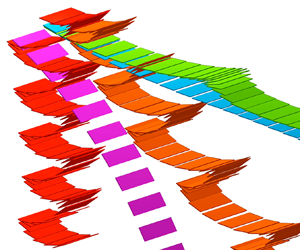
Building on the falling paper system and inspired by paper airplanes in particular, here we explore a rich spectrum of free flight motions achieved by varying the centre of mass location of thin plates. The work of Huang et al. (Reference Huang, Liu, Wang, Wu and Zhang2013) has shown that displacing the centre of mass leads to a variety of flight trajectories, some of which may be reproduced in quasi-steady models. It is also familiar from making paper planes that a good glider requires proper weighting of the front, typically achieved by multiple folds of the leading edge or adding a paper clip (Mander, Dippel & Gossage Reference Mander, Dippel and Gossage1971; Ninomiya Reference Ninomiya1980; Collins Reference Collins2004). We verify this intuition by test flying rectangular sheets of paper with differing degrees of front weighting provided by adding thin metallic tape to one edge. An unweighted, planar sheet undergoes end-over-end tumbling, as shown in figure 1(a). These images are overlaid frames from high-speed video, and the general motions are left to right. Tumbling is also the dominant mode of a flyer formed by adding a small amount of weight that causes the centre of mass to shift somewhat forward, as shown in figure 1(b). Side fins formed by folding up the edges, as shown in the inset, help to maintain in-plane or longitudinal motions. The tape and fins also stiffen the sheet against spanwise and chordwise bending, respectively, and the supplementary movie (available at https://doi.org/10.1017/jfm.2022.89) shows that the sheets do not flex appreciably during flight. Flyers with greater front loading exhibit erratic trajectories involving swoops, climbs, flips and dives, some of which are captured in figure 1(c). Smooth gliding of the paper airplane, shown in figure 1(d), results from ‘just right’ weighting, whereas yet greater front loading produces the steep diving seen in figure 1(e).

Figure 1. Flight motions of paper airplanes with different centre of mass locations. Rectangular sheets of standard copy paper with span  $6\,\textrm {in.} = 15\,\textrm {cm}$ and chord $\ell = 2\,\textrm {in.} = 5\,\textrm {cm}$ are front weighted by differing amounts by applying thin copper tape to the leading edge. Images are superposed frames from high-speed video, and all motions are left to right. (a) Unweighted paper tumbles end over end through air while progressing left to right and descending under gravity. (b) Tumbling of a paper flyer with centre of mass location $\ell _{CM}/\ell = 0.08$, as measured relative to the middle of the chord. Inset: the flyer design includes side fins and tape along the leading edge. (c) Stronger front weighting of $\ell _{CM}/\ell = 0.14$ leads to unsteady motions such as bounding. (d) Gliding of a paper plane with $\ell _{CM}/\ell = 0.24$. (e) Diving for $\ell _{CM}/\ell = 0.31$. The intervals between snapshots are respectively 0.03, 0.03, 0.05, 0.03 and 0.02 s, these values chosen to best convey the motions.
What is the aerodynamics underlying this transformation from ‘plain paper’ to ‘paper plane’? Some aspects of these motivating observations seem well described by classical aerodynamics, e.g. the torque equilibrium needed for gliding at fixed speed and small angle of attack may be explained by the thin airfoil theory prediction that the centre of pressure is located one quarter of the chord length from the leading edge. However, tumbling and other unsteady modes involve time-varying motions that necessitate a dynamical model. Can a single model reproduce all the observed flight modes and thus successfully bridge unsteady and steady behaviours?
In this work, we pursue a quasi-steady model that is directly informed and validated by experiments on the free flight of thin plates with systematically displaced centre of mass locations as well as aerodynamic characterizations of plates in imposed flows. Our ultimate goal is a ‘flight simulator’ that efficiently and accurately solves for the free motions of thin bodies subject to motion-induced fluid forces at moderate to high Reynolds numbers and which reproduces the full spectrum of experimental observations. We present a quasi-steady model that builds on that of Andersen et al. (Reference Andersen, Pesavento and Wang2005b) by replacing torque terms associated with added mass and lift with a term that accounts for the total aerodynamic force (lift and drag) induced by translational motion and which is directly informed by experimental measurements. Simulations of the model that include buoyancy effects and displaced centres of mass successfully reproduce the family of trajectories seen in experiments, both for paper planes in air and thin plates in water. The variety of motions explored include end-over-end tumbling for symmetrically weighted paper in air and back-and-forth fluttering for symmetric plates falling in water, these different base modes expected based on differences in the ratio of solid-to-fluid inertia (Belmonte et al. Reference Belmonte, Eisenberg and Moses1998; Andersen et al. Reference Andersen, Pesavento and Wang2005a). In addition, the experimental systems reveal new modes as the centre of mass is displaced, and the simulations successfully reproduce such motions and explain their origin in the aerodynamics of thin plates. These results suggest that the aerodynamic model and flight simulator are general enough to be further adapted and applied to other problems related to natural and artificial locomotion through fluids.
2. Experiments on the free flight modes of plates in water
Building on our motivating observations of paper airplanes, we next conduct more controlled and systematic experiments on the role of centre of mass (CoM) location for thin plates ‘flying’ through water. This system offers several advantages over paper planes. The flyers are manufactured from plastic that does not flex appreciably during flight, and their shapes are retained even after repeated crash landings, thus ensuring reproducibility of the results. The CoM location can also be more controllably set and systematically varied while keeping the total mass constant. The selected parameters lead to slower flight motions that are more convenient for video recording and tracking while maintaining similar Reynolds numbers  $Re \sim 10^3$ to $10^4$ as for paper airplanes.
The design and construction of the experimental flyers is detailed in figure 2(a). A thin planar plate wing of rectangular planform is laser cut from acrylic plastic sheet, as are two smaller side panels or ‘fins’ into which lead weights are embedded in order to displace the CoM. The fins also serve as aerodynamic stabilizers that resist lateral motions and promote planar or longitudinal flight. We construct 17 such flyers that are identical except for the placement of the paired weights, whose different locations along the chord direction are indicated in figure 2(b). The plate has span length  $s = 8.0\,\textrm {in.} = 20.3\,\textrm {cm}$, chord length $\ell = 1.0\,\textrm {in.} = 2.54\,\textrm {cm}$ and thickness $h =0.060\,\textrm {in.} = 0.15\,\textrm {cm}$. Each fin has length $2.5\,\textrm {in.} = 6.4\,\textrm {cm}$ (at its longest), width $0.5\,\textrm {in.} = 1.27\,\textrm {cm}$ and thickness $0.060\,\textrm {in.} = 0.15\,\textrm {cm}$. Each weight has mass 1 g, and the 17 placements are spaced apart by $1/16\,\textrm {in.} = 0.16\,\textrm {cm}$ spanning from the middle of the chord to a length $1.0\,\textrm {in.} = 2.54\,\textrm {cm}$ towards one edge. These dimensions, along with the densities of water (1.00 g cm $^{-3}$), acrylic (1.18 g cm $^{-3}$) and lead (11.34 g cm $^{-3}$), permit the calculation of relevant quantities such as total mass and volume and hence weight and buoyant force (all identical) as well as the CoM location $\ell _{CM}$ and moment of inertia, which vary across the family of flyers and which will serve as inputs to simulations.

Figure 2. Experiments on the free flight of plates through water. (a) A plate wing and two side fins are laser cut from acrylic plastic, and embedded in the fins are lead weights that serve to displace the CoM. The plate has span length  $s$, chord $\ell$ and thickness $h$. (b) Each of 17 flyers is assembled with the paired weights placed symmetrically along the fins at one of the indicated locations. (c) Buoyancy $\boldsymbol {B}$ acting at the centre of volume (CoV) and weight $\boldsymbol {W}$ acting at the CoM lead to a torque balance about the indicated fulcrum or pivot point, which is defined to be the centre of equilibrium (CoE). (d) Each flyer is released within a large water tank, and in-plane or longitudinal motions are recorded with a video camera.
Each flyer is released in a large glass tank of water, and its free flight motions are recorded using a digital video camera, as shown in the schematic of figure 2(d). The tank has length  $48\,\textrm {in.} = 122\,\textrm {cm}$, width $13\,\textrm {in.} = 33\,\textrm {cm}$ and height $20\,\textrm {in.} = 51\,\textrm {cm}$ and proves to be sufficiently large to observe the long-time behaviour for most of the flyers. To facilitate tracking of the in-plane or longitudinal motions of each flyer, we adhere two markers to the fin nearest the camera and illuminate the front face of the tank with bright lighting. The flyer is released from rest by sliding down a short ramp that is inclined approximately $20^\circ$ below the horizontal, which yields trajectories through the tank that are sufficiently long to determine the terminal behaviours. The planar motions are recorded with a Nikon D610 camera filming at 30 frames per second. A custom MATLAB program tracks the markers and converts these data into position of the CoV (i.e. the mid-chord point) and orientation of the plate. Example movies showing extracted data overlaid on the recorded motions are available as supplementary material.
Repeated trials performed for each body reveal reproducible behaviours that vary systematically across the family of flyers with differing CoM location. The motions extracted from experimental videos for five representative bodies are shown across the top of figure 3(a), where the line segments represent the instantaneous location and orientation of the chord. Arrowheads indicate the direction to which weight is displaced, except for the symmetric body (red) whose weight is placed at the middle of the chord. The symmetric flyer undergoes back-and-forth fluttering, a behaviour well documented in previous studies and consisting of alternating bouts of left- and right-ward gliding swoops punctuated by hard stalls in which the body reverses direction. When the weight is somewhat displaced from the middle, we observe progressive fluttering in which the forward gliding bout is of longer excursion than the backwards, leading to net horizontal motion of the body as it descends. For yet greater weight displacements, the backwards bout disappears altogether, resulting in bounding flight involving bouts of forward gliding interrupted by soft stalls. Further weight displacements eliminate the stalls altogether and produce pure gliding motion that is very nearly steady. Finally, for extreme front weighting, we observe a tendency towards diving in which the body descends straight downward with its weighted edge leading. Independent trials in a deeper tank show edgewise descent is the terminal state.

Figure 3. Trajectories of plate wings from experiments in water (a) and simulations (b) and across flight modes attained by varying the (normalized) CoE location  $\ell _{CE}/\ell$. Five distinct modes are observed: fluttering (red), progressive fluttering (orange-yellow), bounding (green), gliding (blue) and diving (purple-magenta). The plates are shown as arrows whose heads indicate the edge towards which the CoM and CoE have been displaced, except in the symmetric case of $\ell _{CE}/\ell =0$ (red). Snapshots are shown at rate of 6 per second in all cases. The 17 values of $\ell _{CE}/\ell$ explored in experiments are indicated by the arrowheads above the CoE colour bar, with filled symbols corresponding to the 5 trajectories shown above. Simulations cover $\ell _{CE}/\ell$ finely, and hence we indicate with filled arrowheads below the colour bar only the selected values corresponding to the trajectories below. Dashed lines on the colour bar indicate the critical values of $\ell _{CE}/\ell$ separating the modes.
These modes provide detailed points of comparison for flight simulations, whose results shown in figure 3(b) will be discussed in greater detail after the underlying model is explained. The fluid dynamical regime is that of intermediate Reynolds number: the chord  $\ell \approx 2.5$ cm and typical flight speeds $U \approx 5$ to 50 cm s $^{-1}$ yield Reynolds numbers $Re = U \ell / \nu \approx 10^3$ to $10^4$, where $\nu = 10^{-2}\,\textrm {cm}^2\,\textrm {s}^{-1}$ is the kinematic viscosity of water.
Towards classifying these modes and comparing different systems, it will prove useful to define a control parameter related to the CoM displacement but that includes buoyancy effects and thus can be applied generally for flight through different fluids. We introduce the CoE, which is defined as the point along the chord about which the torques associated with weight and buoyancy come into balance under aero- or hydro-static conditions. As shown in figure 2(c) for a flyer of weight  $\boldsymbol {W}$ and total buoyant force $\boldsymbol {B}$, the CoE distance from the middle of the plate or the CoV can be calculated to be $\ell _{CE} = \ell _{CM} |\boldsymbol {W}| / (|\boldsymbol {W}| - |\boldsymbol {B}|)$. For dense solids such as paper planes in air, $|\boldsymbol {W}| \gg |\boldsymbol {B}|$ and $\ell _{CE} \approx \ell _{CM}$. For our underwater flyers, however, buoyancy is considerable and the CoE deviates significantly from the CoM. The values of the CoE location $\ell _{CE}/\ell$ relative to the chord explored in the experiments are indicated by arrowheads above the colour bar in figure 3, with filled symbols corresponding to the trajectories above. The vertical dashed line segments on the upper portion of the CoE colour bar indicate the approximate boundaries between the modes. These experimental observations will serve to validate the model presented in later sections.
3. Static torque measurements and aerodynamic characterization
We next pursue an experimental characterization of the fluid dynamical forces and torque on plates fixed within imposed flows, this information to be used to inform our quasi-steady model. Particular attention is placed on pitching torque and its dependence on angle of attack, since added mass torque models tend to over-predict experimental measurements, as noted in Pesavento & Wang (Reference Pesavento and Wang2004) and Andersen et al. (Reference Andersen, Pesavento and Wang2005b). Added mass effects included in previous studies derive from the Kirchhoff equations governing the motion of an object in potential (inviscid) flow with zero circulation. Viscous flows involve vortex shedding that redistributes pressure and significantly modifies torques, thus necessitating new models. Here, we present an approach that allows for the extraction of the relevant force and torque characteristics from experimental torque measurements about different points of rotation and for varying angles of attack. This procedure furnishes the total force associated with fluid dynamic pressure and thus its decomposition into lift and drag. The total torque can then be expressed as the total force acting at a centre of pressure location along the chord.
3.1. Experimental torque measurements
The first step involves experiments for measuring the flow-induced torque on plates, which we carry out using a spring balance system and water tunnel. The apparatus shown schematically in figure 4(a) has been successfully employed and thoroughly described in previous studies (Amin et al. Reference Amin, Huang, Hu, Zhang and Ristroph2019; Sanaei et al. Reference Sanaei, Sun, Li, Peskin and Ristroph2021). Here, we review the basic components and operating procedures and provide relevant parameters for our characterization of plates. Laminar flow is provided by a recirculating water tunnel whose test section measures  $6\,\textrm {in.} \times 6\,\textrm {in.}$ ( $15\,\textrm {cm} \times 15\,\textrm {cm}$) in cross-section and 17 inches (43 cm) in length. Each plate is loaded vertically in the test section, and the use of stainless steel ensures minimal flexing. The plates measure $6\,\textrm {in.} \times 1\,\textrm {in.} \times 0.03\,\textrm {in.}$ or, equivalently, $(s = 15\,\textrm {cm}) \times (\ell = 2.5\,\textrm {cm}) \times (h = 0.076\,\textrm {cm})$ in span, chord and thickness. They nearly span the height of the tunnel. We consider the family of plates identical except for the location $\ell _p$ along the chord of the support rod or pivot point, which is the axis of rotation about which the torques are measured and which we will later associate with $\ell _{CE}$ in the context freely flying plates. A two-dimensional schematic defining relevant quantities is shown in figure 4(b). The support rod extends upward out of the tunnel, where it is held in low friction, rotary ball bearings. The rod is connected to a coil or torsion spring whose other end is fixed to a housing (not shown in the figure) that is rigidly attached to the tunnel lid. Also not shown is a viscous dashpot that strongly suppresses vibrations of the plate triggered by hydrodynamic fluctuations such as vortex shedding.

Figure 4. Experimental characterization of flow-induced torques. (a) Apparatus for measuring pitching torque on plates in imposed flows. The plate is inserted vertically in the test section of a laminar flow water tunnel, and a torsion spring balance is used to measure torques. The mounting shaft is secured in low friction ball bearings (not shown) and connected to a coil spring that loads slightly under flow-induced torque. Slight angular deflections lead to amplified displacements along a ruler for a laser beam that reflects off a small mirror on the shaft. Calibration is used to convert beam displacement to torque. (b) Chordwise view of the plate and definitions of relevant quantities: flow speed  $U$, attack angle $\alpha$ and pitching torque $\tau$ for a given pivot point location $\ell _p$. Not indicated are the chord $\ell$ and span $s$ lengths. (c) The measured torque is normalized to form the torque coefficient $C_{\tau } = 2 \tau / \rho U^2 s \ell ^2$ across $\alpha$ and $\ell _p/\ell$, with tested values of the latter marked on the colour bar. (d) Plots of the measured torque coefficient $C_{\tau }$ vs $\ell _p/\ell$ for selected values of $\alpha$ and their best-fit lines.
When flow is initiated, any torque exerted on the plate causes it to rotate through a slight angle ( $< 5^{\circ }$) and loads the spring. This deflection is amplified for measurement by reflecting a laser beam off a small mirror mounted on the support rod. A long path of the beam, achieved compactly with a second mirror, ensures measurably large excursions of the beam along a long ruler. Calibration using a mass–string–pulley system yields the conversion of the beam displacement to torque. Here, we report on 9 plates with different values of the normalized pivot point location $\ell _p/\ell \in [0,0.65]$, where $\ell _p/\ell = 0$ corresponds to the middle of the chord and $\ell _p/\ell = 0.5$ is at the leading edge. For each plate of a given $\ell _p/\ell$, we sweep through angles of attack $\alpha$ while measuring the beam displacement and thus torque $\tau$ at each angle. These data are recast into the torque coefficient $C_{\tau } = \tau / (\rho U^2 s \ell ^2 / 2)$, a non-dimensionalization that removes the expected dependencies on fluid density $\rho$, flow speed $U$ and plate dimensions based on high-Re pressure forces. We impose flow speeds that decrease from 15 to 7 cm s $^{-1}$ for the plates of increasing $\ell _p$ in order to yield convenient beam displacements, these values yielding Reynolds numbers $Re = 2000$ to 4000 within the range explored in the free flight experiments.
The data gathered can be collectively summarized as  $C_{\tau }(\ell _p/\ell,\alpha )$. In figure 4(c), we display curves $C_{\tau }(\alpha )$ for different values of $\ell _p/\ell$. The markers indicate measured values, and the solid curves are spline fits to be used in the analysis that follows.
3.2. Inferring lift, drag and torque coefficients
We next outline a procedure that uses the torque data to infer the total force coefficient, its decomposition into lift and drag coefficients and the centre of pressure location, all of which vary with  $\alpha$. Because of the thin and flat geometry, the torque derives from the pressure difference $p (x)$ across the plate, whose variation with the chordwise coordinate $x$ is not known a priori. Hence the torque is given by
 \begin{align} \tau (\ell_p,\alpha) =\int (x-\ell_p) p (x,\alpha) s\,{{\rm d}x} &= \int x p (x,\alpha) s\,{{\rm d}x} - \ell_p \int p (x,\alpha) s\,{{\rm d}x} \nonumber\\ &= \tau_0 (\alpha) - \ell_p F(\alpha), \end{align}
where the integrals are over the length of the chord ( $-\ell /2$ to $\ell /2$) and $s$ is the span length. The two integrals that arise are associated with the torque $\tau _0$ about the CoV (middle of the plate) and the total normal force $F$ on the plate, respectively,
 \begin{equation} \tau_0 (\alpha) = \tau (\ell_p=0,\alpha) = \int x p (x,\alpha) s\,{{\rm d}x} \quad\textrm{and}\quad F(\alpha) = \int p (x,\alpha) s\,{{\rm d}x}, \end{equation}
these quantities depending on  $\alpha$ but not on $\ell _p/\ell$. Converting to dimensionless force and torque coefficients by normalizing by $\rho U^2 s \ell /2$ and $\rho U^2 s \ell ^{2} /2$, respectively, yields
 \begin{equation} C_{\tau} (\ell_p/\ell,\alpha) = C_{\tau_0} (\alpha) - (\ell_p / \ell ) C_{F}(\alpha). \end{equation}
Thus, for a given  $\alpha$, plotting $C_\tau (\ell _p/\ell,\alpha )$ vs $\ell _p/\ell$ is expected to yield a line whose slope has magnitude given by the total force coefficient $C_{F}(\alpha )$. This is borne out in figure 4(d), where we display as markers the data extracted from the spline fits of figure 4(c) for selected values of $\alpha$. Note that, whereas in figure 4(c) we take the domains to be $\ell _p/\ell \geq 0$ and $\alpha \in [0^\circ,180^\circ ]$, in figure 4(d) we allow $\ell _p/\ell \in \mathbb {R}$ to be negative and restrict $\alpha \in [0^\circ,90^\circ ]$, this change being permitted by the symmetries of the plate. The lines are linear regression fits whose slopes yield the total force coefficient $C_F(\alpha ) = F(\alpha )/(\rho U^2 s \ell / 2)$ shown as the solid curve in figure 5(a).

Figure 5. The dependence of aerodynamic coefficients on angle of attack  $\alpha$, as extracted from experiments (solid curves) and their model forms (dashed). (a) The force coefficient $C_{F}$ associated with pressure forces and thus assumed to act normal to the plate. (b) The torque coefficient $C_{\tau _0}$ about the CoV. (c) The lift $C_{L}$ and drag $C_{D}$ coefficients formed by decomposing the total force into components perpendicular and parallel to the flow direction. (d) The centre of pressure location represents the effective site at which the force acts in giving rise to the CoV torque: $\ell _{CP}/\ell = C_{\tau _0} / C_{F}$.
The lift and drag coefficients are then readily extracted as components of the force perpendicular and parallel to the wind vector, respectively,
 \begin{equation} C_L (\alpha) = C_F (\alpha) \cos \alpha \quad\textrm{and}\quad C_D (\alpha) = C_F (\alpha) \sin \alpha. \end{equation}
The resulting curves are displayed in figure 5(c). Note that these forms represent the lift and drag components of the force normal to the plate. At high Reynolds numbers and sufficiently high  $\alpha$, one expects normal or pressure forces to dominate over tangential forces or skin friction, and so these forms are good approximations to the total lift and drag. The coefficient curves inferred by our procedure are in qualitative agreement with direct force measurements conducted for similar but somewhat different plate geometries and Reynolds numbers (Pelletier & Mueller Reference Pelletier and Mueller2000; Okamoto & Azuma Reference Okamoto and Azuma2011; Shields & Mohseni Reference Shields and Mohseni2012).
Finally, the torque is related to the centre of pressure location
 \begin{equation} \ell_{CP} (\alpha) = \frac{\int x p (x,\alpha)\,{{\rm d}x}}{\int p (x,\alpha)\,{{\rm d}x}} = \frac{\tau_{0}(\alpha)}{F(\alpha)} = \frac{\ell C_{\tau_0} (\alpha)}{C_{F}(\alpha)}, \end{equation}
whose definition in the first equality is analogous to quantities such as CoM. The value of  $\ell _{CP}$ indicates the distance from the middle of the plate at which the normal force effectively acts. Extracting $C_{\tau _0}(\alpha )$ from the vertical intercepts of the curves in figure 4(d) yields the solid curve of figure 5(b) and thus the normalized $\ell _{CP}(\alpha )/\ell = C_{\tau _0}(\alpha ) / C_{F}(\alpha )$ shown in figure 5(d).
The above procedure can be validated by comparing the experimentally measured  $C_{\tau } (\ell _p/\ell,\alpha )$ with that inferred via (3.3) with the extracted forms of $C_{\tau _0}$ and $C_{F}$. The former data are shown as markers in figure 6(a) and the latter by the curves, and the relevant trends can be seen to be captured well. Here, the colouring indicates $\ell _p/\ell$ and follows the colour bar presented in figure 4(c). The extracted $C_L(\alpha )$, $C_D(\alpha )$ and $\ell _{CP}(\alpha )/\ell$ curves constitute a complete characterization of the aerodynamic forces and pitching torque under static conditions, and these quantities inform the model presented in subsequent sections.

Figure 6. Equilibrium postures and their static stability across different points of rotation. (a) Extracted torque coefficients (curves) compared with measurements (markers). The colouring indicates the pivot location  $\ell _p/\ell$ and follows the colour bar of figure 5(c). Equilibrium angles of attack are associated with $C_\tau = 0$ and include $\alpha = 0^\circ$ and $\alpha = 180^\circ$ for all $\ell _p$ as well as non-trivial solutions at intermediate $\alpha$ for some curves. (b) Magnified view of low- $\alpha$ torque response corresponding to the dashed box of (a). The equilibrium orientation $\alpha = 0$ changes slope as $\ell _p$ increases. The non-trivial equilibria for $\alpha > 0$ occur at decreasing $\alpha$ for increasing $\ell _p$, as shown here for two such solutions (green and blue boxes). (c) Stability derivative $d C_\tau / d \alpha$ vs $\ell _p/\ell$ for all equilibria. Positive values imply static instability, while negative values are stable. The posture $\alpha = 180^\circ$ is always unstable, whereas $\alpha = 0^\circ$ transitions from unstable to stable at a critical $\ell _p/\ell \approx 0.3$. The non-trivial equilibria are mostly stable. (d) Static stability map showing the dependence of equilibrium attack angles on pivot location. Stable or attracting orientations are shown as solid curves and unstable or repelling postures are dotted.
3.3. Static equilibria and their stability
The extracted torque profiles convey important information about the equilibrium orientations of the plate, which correspond to  $C_{\tau } = 0$, as well as their stability, which relates to the slope $\text {d} C_{\tau } / \text {d} \alpha$. The edgewise orientations $\alpha = 0^\circ$ and $\alpha = 180^\circ$ are equilibria for all $\ell _p/\ell$, as is consistent with the symmetry of these postures. For a plate supported about its middle, i.e. $\ell _p/\ell = 0$ represented by the red curve in figure 6(a), both $\alpha = 0^\circ$ and $\alpha = 180^\circ$ are unstable in the static sense: $\text {d} C_{\tau } / \text {d} \alpha > 0$ and thus small perturbations are expected to grow. In contrast, the broadside-on posture of $\alpha = 90^\circ$ is an equilibrium that is statically stable since $\text {d} C_{\tau } / \text {d} \alpha < 0$. As $\ell _p/\ell$ increases, this single stable orientation moves to lower values of $\alpha$ until $\ell _p/\ell \approx 0.3$ (dark purple curve in figure 6a), beyond which the stable orientation remains at $\alpha = 0^\circ$. Hence, the equilibrium point $\alpha = 0^\circ$ transitions from unstable to stable near $\ell _p/\ell = 0.3$.
For a closer inspection of the low- $\alpha$ response, we show a zoomed-in view of $C_{\tau } (\ell _p/\ell,\alpha )$ in figure 6(b), which corresponds to the dashed box of (a). Their odd symmetry allows the curves to be extended to negative $\alpha$ (faded), which helps to show the slopes at $\alpha = 0^\circ$. The equilibrium posture $\alpha = 0^\circ$ undergoes a transition from positive to negative slope and thus from unstable to stable. The zero crossings for $\alpha > 0^\circ$ for the green and blue curves are marked by boxes and correspond to non-trivial equilibria whose negative slopes indicate stability. Those of particularly low $\alpha$, an example of which is the blue curve with $\ell _p/\ell = 0.24$, correspond to the gliding mode observed in the flight experiments of figure 3.
The inferences of stability given above can be confirmed by assessing the stability derivative  $\text {d} C_{\tau } / \text {d} \alpha$ across all equilibria, as shown in figure 6(c). Here, the three branches correspond to $\alpha = 0^\circ$, $\alpha = 180^\circ$ and the non-trivial equilibria of intermediate $\alpha$. Noting again that the sign of the derivative indicates stability with negative being stable, it can be seen that $\alpha = 180^\circ$ is always unstable, while $\alpha = 0^\circ$ transitions from unstable to stable as $\ell _p/\ell$ increases. (Due to symmetries of the plate, the $\alpha = 180^\circ$ curve for $\ell _p/\ell >0$ can be interpreted as a reflection of the $\alpha = 0^\circ$ curve extended to $\ell _p/\ell <0$.) The non-trivial equilibria that arise for sufficiently small $\ell _p/\ell < 0.3$ are mostly stable, with a weakly unstable solution appearing around $\ell _p/\ell = 0.13$.
The locus of all equilibrium points and their stability is summarized in figure 6(d). Solid and dotted curves represent the stable (attracting) and unstable (repelling) equilibria, respectively. For each value of  $\ell _p/\ell$, the arrows convey the expected evolution of $\alpha$ away from unstable branches and towards stable branches. The trivial equilibrium $\alpha = 0^\circ$ undergoes a change from unstable to stable while $180^\circ$ is always unstable. The curve shows how the non-trivial equilibria move towards lower values of $\alpha$ as $\ell _p/\ell$ increases and eventually reach $\alpha = 0^\circ$ near $\ell _p/\ell = 0.3$, this being associated with a pitchfork-like bifurcation in the map. Note that this curve $\alpha (\ell _{p}/\ell )$ representing non-trivial equilibria is simply the inverse of the curve $\ell _{CP} (\alpha ) / \ell$ shown in figure 5(d), which is explained by the fact that $\ell _{p} = \ell _{CP}$ satisfies the zero torque condition for equilibrium.
The equilibria and their static stability can be related to the flight observations of figure 3. Edgewise diving (purple and magenta) corresponds to the attractor at  $\alpha = 0^\circ$ for sufficiently high $\ell _p/\ell > 0.3$. Gliding (blue) corresponds to the attractor at small but non-zero $\alpha$, which our free flight experiments show to be the mode attained for $\ell _p/\ell \in (0.22,0.29)$. The bounding mode (green) as well as progressive fluttering (orange and yellow) and fluttering (red) have attractors at larger values of $\alpha$, but these statically stable postures are apparently dynamically unstable in free flight and give rise to oscillatory motions. The transition from gliding to bounding is reminiscent of a Hopf bifurcation in which a stable fixed point gives way to limit cycle oscillations.
4. A quasi-steady model framework
Our model describes the free motions of a plate subject to gravitational and aero- or hydro-dynamic forces at moderate to high Reynolds numbers. The general framework and nomenclature largely follow those of Andersen et al. (Reference Andersen, Pesavento and Wang2005b). Our modifications account for displaced CoM and include revisions to the fluid dynamical force and torque model. We consider the two-dimensional (2-D) setting of a thin plate of mass  $m$ and rectangular cross-section, with chord length $\ell$ and thickness $h \ll \ell$ defined according to figure 7(a). The mass is distributed such that the CoM is displaced from the CoV by a distance $\ell _{CM} \geq 0$. The moment of inertia about the CoM is given by $I = \frac {1}{12}m(h^2+\ell ^2) + m \ell ^{2}_{CM}$ per the parallel axis theorem. This form applies to rotations about the CoM of a plate of homogeneous density and does not explicitly account for the specific manner (such as adding weights) by which the displaced CoM is achieved. This issue will be addressed in more detail in § 6 where we simulate the conditions relevant to the free flight experiments presented in § 2.

Figure 7. Definitions of model parameters. (a) A thin plate of chord length  $\ell$, thickness $h \ll \ell$ and CoM displacement $\ell _{CM}$. (b) The CoE location $\ell _{CE}$ as defined by the balance of weight and the buoyant force. (c) The aerodynamic force $F$ acts at a distance $\ell _{CP}$ from the CoV. (d) Kinematic parameters and reference frames. The laboratory frame $(x,y)$ is fixed and the frame $(x',y')$ rotates with the plate. The instantaneous orientation angle $\theta$ is positive as shown. The angle of attack $\alpha$ is measured between the CoV velocity vector $\boldsymbol {v}^{CV}$ and the $x'$-axis, with $\alpha <0$ as shown. (e) Force diagram. The weight $\boldsymbol {W}$ and buoyant force $\boldsymbol {B}$ are directed downward and upward, respectively, while lift $\boldsymbol {L}$ is perpendicular to $\boldsymbol {v}^{CV}$ and drag $\boldsymbol {D}$ is anti-parallel.
Under aero/hydro-static conditions, the weight  $\boldsymbol {W}$ and buoyant force $\boldsymbol {B}$ lead to a CoE location $\ell _{CE} = \ell _{CM} |\boldsymbol {W}| / (|\boldsymbol {W}| - |\boldsymbol {B}|)$, as shown in figure 7(b). This is essentially the CoM location for dense solids in air (for which $|\boldsymbol {W}| \gg |\boldsymbol {B}|$) but deviates significantly for the underwater flyers of the experiments reported in § 2. The CoE location proves useful as the reference point against which the point of action of the fluid dynamic forces should be compared. An ideal plate of solid density $\rho _s$ in a fluid of density $\rho _f$ has $\ell _{CE} = \ell _{CM} \rho _s / (\rho _s - \rho _f)$. When simulating our free flight experiments, the more general formula above will be used to account for the added weights and side fins.
We assume the aero/hydro-dynamics is that of a simple plate moving within a fluid of density  $\rho _f$. The aerodynamic force $F$ and the centre of pressure location $\ell _{CP}$, as defined in figure 7(c), vary with the plate motion according to the model described in detail below. The instantaneous position of the CoM in the fixed or laboratory reference frame is denoted $(x,y)$, as shown in figure 7(d). The orientation is given by the angle $\theta$ measured relative to gravity, defined such that counterclockwise rotations are positive.
A reference frame  $(x',y')$ that co-rotates with the plate, as shown in figure 7(d), is convenient for expressing the equations of motion. The velocity of the CoM $\boldsymbol {v}^{CM} = \boldsymbol {v}$ has components in the two frames that are related by the transformations $v_{x} = v_{x'} \cos \theta - v_{y'} \sin \theta$ and $v_{y} =v_{x'} \sin \theta + v_{y'} \cos \theta$. The angular velocity of the plate is $\omega =\dot {\theta }$. While the rigid body dynamics is best described in terms of the CoM motion, aerodynamic terms will involve the CoV velocity $\boldsymbol {v}^{CV}$, whose primed frame components $(v^{CV}_{x'},v^{CV}_{y'}) = (v_{x'},v_{y'}-\omega \ell _{CM})$ differ from the CoM velocity $(v^{CM}_{x'},v^{CM}_{y'})=(v_{x'},v_{y'})$ due to rotation.
The planar longitudinal dynamics of the plate is described by three Newton–Euler equations relating translational and rotational accelerations to forces and torques and which include the effects of gravity, buoyancy and aerodynamics. A force diagram is shown in figure 7(e). The fluid dynamical forces are described by a quasi-static model that may be decomposed into several terms. The equations of motion in the co-rotating (primed) frame are
 $$\begin{gather} m \dot{v}^{CM}_{x'} + m_{11} \dot{v}^{CV}_{x'} = m \omega v^{CM}_{y'} + m_{22}\omega v^{CV}_{y'} + L_{x'} + D_{x'} - m'g \sin \theta, \end{gather}$$
 $$\begin{gather}m \dot{v}^{CM}_{y'} + m_{22} \dot{v}^{CV}_{y'} ={-}m \omega v^{CM}_{x'} - m_{11}\omega v^{CV}_{x'} + L_{y'} + D_{y'} - m'g \cos \theta, \end{gather}$$
 $$\begin{gather}(I+I_{a}) \dot{\omega} = \tau_T + \tau_R + \tau_B, \end{gather}$$
where all masses, moments, forces and torques should be understood as being per unit span for this 2-D setting. The rigid body dynamics involves the solid mass  $m$ and the CoM acceleration terms proportional to $\dot {\boldsymbol {v}}^{CM}$ and $\omega \boldsymbol {v}^{CM}$. The latter appear as the first terms on the right-hand sides of (4.1) and (4.2) and are due to the co-rotating reference frame. Gravity and buoyancy give rise to the last term in each equation. Fluid dynamical effects include the added mass force terms with $m_{11}$ and $m_{22}$, whose forms follow the derivations of Sedov (Reference Sedov1965) as used in Andersen et al. (Reference Andersen, Pesavento and Wang2005b). They involve the CoV acceleration with translational and rotational contributions proportional to $\dot {\boldsymbol {v}}^{CV}$ and $\omega \boldsymbol {v}^{CV}$, respectively. Additional aerodynamic terms involve lift $\boldsymbol {L}$, drag $\boldsymbol {D}$ and associated torques $\tau _T$ and $\tau _R$ due to translation and rotation of the plate.
The system above should be compared with the analogous equations (6.1)–(6.3) in Andersen et al. (Reference Andersen, Pesavento and Wang2005b). Our modifications, which are spelled out in detail below, are intended to achieve several goals. (i) To extend the force model of Andersen et al. (Reference Andersen, Pesavento and Wang2005b) to include asymmetric weighting of  $\ell _{CM} > 0$. This is done by associating all fluid dynamical force terms (added mass, lift and drag) with the CoV velocity $\boldsymbol {v}^{CV}$ and all rigid body dynamical terms with the CoM velocity $\boldsymbol {v}^{CM}$. (ii) To extend the torque model to include asymmetric weighting. This introduces a buoyancy torque $\tau _B$. Further, the rotational drag-based torque $\tau _R$, which is called $\tau ^v$ in Andersen et al. (Reference Andersen, Pesavento and Wang2005b), must be computed about the CoM. (iii) To modify the lift and drag coefficients that will appear in the $\boldsymbol {L}$ and $\boldsymbol {D}$ terms to more accurately account for attached flow at low $\alpha$ and separated flow at high $\alpha$. The following section will provide details of how we specify model force coefficients that are informed by experiments. (iv) To address the finding in previous works that the added mass torque significantly over-predicts experimental measurements (Pesavento & Wang Reference Pesavento and Wang2004; Andersen et al. Reference Andersen, Pesavento and Wang2005b). We remove the added mass torque and replace it with the term $\tau _T$ that derives from the lift, drag and centre of pressure during translation. We view the points (i) and (ii) above as essential to satisfying the basic physics of the new system with displaced CoM, whereas (iii) and (iv) are modelling choices intended to improve accuracy.
The system of (4.1)–(4.3) together with the coordinate transformations can be expressed as a system of first-order ordinary differential equations in the state variables  $(x,y,\theta,v_{x'},v_{y'},\omega )$ by eliminating $\boldsymbol {v}^{CV}$ in favour of $\boldsymbol {v}^{CM}=\boldsymbol {v}$
 $$\begin{gather} \dot{x} = v_{x'} \cos \theta - v_{y'} \sin \theta, \end{gather}$$
 $$\begin{gather}\dot{y} = v_{x'} \sin \theta + v_{y'} \cos \theta, \end{gather}$$
 $$\begin{gather}\dot{\theta} = \omega, \end{gather}$$
 $$\begin{gather}(m+m_{11}) \dot{v_{x'}} = (m+m_{22}) \omega v_{y'} - m_{22} \omega^{2} \ell_{CM} + L_{x'} + D_{x'} - m'g \sin \theta, \end{gather}$$
 $$\begin{gather}(m+m_{22}) \dot{v_{y'}} ={-}(m+m_{11}) \omega v_{x'} + m_{22} \dot{\omega} \ell_{CM} + L_{y'} + D_{y'} - m'g \cos \theta, \end{gather}$$
 $$\begin{gather}(I+I_{a}) \dot{\omega} = \tau_T + \tau_R + \tau_B. \end{gather}$$
The fifth equation (4.8) has  $\dot {\omega }$ on the right-hand side, but the sixth equation (4.9) recast as $\dot {\omega } = (\tau _T + \tau _R + \tau _B)/(I+I_{a})$ can be used to arrive at a system with only state variables on the right. Looking ahead to our simulations, this system can be numerically integrated in time using, say, MATLAB's ode45 solver to yield the laboratory frame CoM trajectory $(x,y,\theta )$ as well as any other desired quantities.
Analytical expressions are not available for the added mass coefficients of rectangular-section plates of finite span, and we assume forms for infinitesimally thin plates:  $m_{11} = 0$ and $m_{22} = {\rm \pi}\rho _f \ell ^2 / 4$. The added moment of inertia about the CoM is $I_a = I_{a} (\ell _{CM}=0) + m_{22} \ell ^{2}_{CM} = {\rm \pi}\rho _f \ell ^4 [1+8 (2\ell _{CM} / \ell )^2] / 128$, as computed using the thin-plate approximation and the parallel axis theorem.
The last terms of (4.7) and (4.8) are the primed frame components of buoyancy reduced weight, where  $m' = (\rho _s -\rho _f) h \ell$ for a solid plate of (homogeneous) density $\rho _s$. The last term in (4.9) is the buoyancy induced torque, $\tau _B = - \rho _f g h \ell \ell _{CM} \cos \theta$, which is associated with the CoM being displaced a distance $\ell _{CM}$ from the CoV. The expressions for these buoyancy terms are for a simple 2-D plate of cross-sectional area $h \ell$. Appropriate modifications are given in § 6 when simulating the experimental flyers, which have additional fins and weights.
The remaining terms represent aero- or hydro-dynamic forces and torques that are induced by translation or rotation of the plate through the fluid and which are modelled by lift, drag and the associated torques. These terms depend on angle of attack  $\alpha \in [-{\rm \pi},{\rm \pi} ]$, which is defined to be the angle of the CoV velocity vector $\boldsymbol {v}^{CV}$ relative to the $x'$ axis of the plate, as shown in figure 7(d). Hence, $\tan \alpha = v^{CV}_{y'}/v^{CV}_{x'} = (v_{y'}-\omega \ell _{CM})/v_{x'}$. Lift and drag have terms associated with translational motions that depend quadratically on the CoV speed, with lift directed perpendicular to the CoV velocity vector and drag directed anti-parallel, as shown in figure 7(e). The lift also has a rotational or Magnus-like term that depends on the product of translational and rotational speeds. The vector forces can be expressed as
 $$\begin{gather} \boldsymbol{L_T} = \tfrac{1}{2} \rho_f \ell C_{L}(\alpha) \sqrt{v^2_{x'} + (v_{y'}-\omega \ell_{CM})^2} ( v_{y'}-\omega \ell_{CM},-v_{x'} ) \end{gather}$$
 $$\begin{gather}\boldsymbol{L_R} ={-}\tfrac{1}{2} \rho_f \ell^2 C_{R} \omega ( v_{y'}-\omega \ell_{CM},-v_{x'} ) \end{gather}$$
 \begin{gather} \hspace{-23.1pc}\boldsymbol{L} = \boldsymbol{L_T} + \boldsymbol{L_R} \nonumber\\ = \tfrac{1}{2} \rho_f \ell \left[ C_{L}(\alpha) \sqrt{v^2_{x'} + (v_{y'}-\omega \ell_{CM})^2} - \ell C_R \omega \right] ( v_{y'}-\omega \ell_{CM},-v_{x'}) \end{gather}
 \begin{gather} \boldsymbol{D} ={-}\tfrac{1}{2} \rho_f \ell C_{D}(\alpha) \sqrt{v^2_{x'} + (v_{y'}-\omega \ell_{CM})^2} ( v_{x'},v_{y'}-\omega \ell_{CM} ). \end{gather}
Here,  $C_D$, $C_L$ and $C_R$ are the order-one drag, translational lift and rotational lift coefficients. As discussed in detail in the following section, we will assume a constant $C_R$ and functional forms for $C_{D}(\alpha )$ and $C_{L}(\alpha )$ that are good matches to our experimental measurements of the flow-induced torque.
The torque term  $\tau _T$ of the sixth dynamical equation represents the effect of translational lift and drag acting at a centre of pressure location $\ell _{CP}(\alpha )$ that may in general be different from $\ell _{CM}$, as shown in figure 7(c). Only the components of these forces along $y'$ contribute
 \begin{align} \tau_T &= (L_{Ty'} + D_{y'})(\ell_{CP} - \ell_{CM}) \nonumber\\ &={-}\tfrac{1}{2} \rho_f \ell \sqrt{v^2_{x'} + (v_{y'}-\omega \ell_{CM})^2} \left[ C_{L} v_{x'} + C_{D} (v_{y'}-\omega \ell_{CM}) \right] (\ell_{CP} - \ell_{CM}), \end{align}
where the dependence of  $C_L$, $C_D$ and $\ell _{CP}$ on $\alpha$ have been suppressed. The functional form for the centre of pressure location $\ell _{CP}(\alpha )$ is specified in the following section.
The torque term  $\tau _R$ in the third dynamical equation is intended to capture the aerodynamic resistance to rotations. Following the dissipative torque approximation of Andersen et al. (Reference Andersen, Pesavento and Wang2005b), we calculate an expression for this term by considering a plate under steady rotation about the CoM and without translation, where the drag is integrated along the chord in a blade-element sense
 \begin{equation} \tau_R ={-}\frac{1}{128} \rho_f \ell^4 C^{{\rm \pi}/2}_{D} \omega |\omega| \left[\left( \frac{2 \ell_{CM}}{\ell} + 1 \right)^4 \pm \left( \frac{2 \ell_{CM}}{\ell} - 1 \right)^4 \right]. \end{equation}
The appearance of  $C^{{\rm \pi} /2}_{D} = C_{D}(\alpha ={\rm \pi} /2)$ reflects the fact that pure rotation involves only broadside-on motion of each segment along the chord. The plus sign applies for $2 \ell _{CM} / \ell \leq 1$, i.e. when the CoM lies within the plate, and the negative sign applies for $2 \ell _{CM} / \ell > 1$, i.e. when the CoM lies beyond the edge, as is the case for the most front-weighted plates explored in the experiments of figure 3. With this term specified, the sixth equation (4.9) in the dynamical system is complete.
5. Aerodynamic coefficients and parameters in the model
We next specify the angle-of-attack dependence of the aerodynamic force coefficients and parameter values employed in the model. The general strategy taken here is semi-theoretical and semi-empirical, i.e. we employ formulas informed by theory wherever possible but with prefactors and other parameter values informed by experiments. We also wish to account for differing characteristics for laminar or attached flow vs stalled or separated flow.
As noted in Andersen et al. (Reference Andersen, Pesavento and Wang2005b), the functional form of the rotational lift term in the system of (4.11) follows that calculated by Munk (Reference Munk1925) for a pitching plate at zero angle of attack, in which case the coefficient value is shown to be  $C_R = {\rm \pi}$. We follow the assumption of Andersen et al. (Reference Andersen, Pesavento and Wang2005b) that the general form holds for all $\alpha$, and we employ the value $C_R = 1.1$ that was empirically determined to apply well to thin plates.
The translational coefficients  $C_{L}(\alpha )$ and $C_{D}(\alpha )$ as well as the centre of pressure location $\ell _{CP}(\alpha )$ are all assumed to depend on $\alpha$. Because we are concerned with rectangular plates that are symmetric both up–down and front–back, it is sufficient to specify these parameters over the range $\alpha \in [0,{\rm \pi} /2]$. As shown in figure 8, if lift, drag and the point of action of these forces is specified for $\alpha \in [0,{\rm \pi} /2]$, then one can invoke symmetries to construct the force diagrams over the entire range $\alpha \in [-{\rm \pi},{\rm \pi} ]$.

Figure 8. Diagram of lift  $\boldsymbol {L}$ and drag $\boldsymbol {D}$ for varying angle of attack $\alpha$. If the aerodynamic forces and their location are specified in the range $\alpha \in [0,{\rm \pi} /2]$ (b), the symmetries of a plate allow these characteristics to be determined for all $\alpha \in [-{\rm \pi},{\rm \pi} ]$.
Taking up the case of translational lift, the laminar flow condition expected at low angles of attack  $\alpha$ is described by the classical Kutta–Joukowski theory for thin airfoils that predicts a lift coefficient proportional to $\sin \alpha$, as has been confirmed experimentally for symmetric foils (Anderson Reference Anderson2010). For stalled conditions at higher $\alpha$, the free streamline theory for fully separated flow predicts that the net aerodynamic force is directed normal to a plate (Wu Reference Wu1955; Lamb Reference Lamb1993; Sefat & Fernandes Reference Sefat and Fernandes2011), implying that lift varies in proportion to $\sin 2\alpha$. This form is also consistent with previous results from experiments and numerical simulations (Wang et al. Reference Wang, Birch and Dickinson2004; Sefat & Fernandes Reference Sefat and Fernandes2011). Our model smoothly combines these behaviours, yielding the form
 $$\begin{gather} \tilde{C}_{L}(\alpha) = \tilde{f}(\alpha) \cdot C^{1}_{L} \sin \alpha + [1-\tilde{f}(\alpha)] \cdot C^{2}_{L} \sin 2\alpha \quad \alpha \in [0,{\rm \pi}/2] \end{gather}$$
 $$\begin{gather}\tilde{f}(\alpha) = \frac{1-\tanh [ (\alpha - \alpha_0 ) / \delta ]}{2} \quad \alpha \in [0,{\rm \pi}/2]. \end{gather}$$
Here, the tilde symbol over the functions is used to indicate their limited domain  $\alpha \in [0,{\rm \pi} /2]$. The parameter values $C^{1}_{L} = 5.2$ and $C^{2}_{L} = 0.95$ are chosen to yield good agreement with the measurements of figure 5(c) for the lift on plates fixed in imposed flows. The former value is fairly close to the prefactor of $2 {\rm \pi}\approx 6.3$ predicted by Kutta–Joukowski theory for thin airfoils at low angles of attack (Anderson Reference Anderson2010). The purpose of the function $\tilde {f}(\alpha )$, which is plotted in figure 9(a) for $\alpha \in [0,{\rm \pi} /2]$ as the heavier portion of the curve, is to select either the laminar or separated (stalled) regime, where $\alpha _0 = 14^\circ$ is the critical angle of attack at stall and $\delta = 6^\circ$ determines the smoothness of the transition. These values are selected to yield acceptable agreement with our experimental measurements. Smaller $\delta$ yields a more abrupt transition and larger $\delta$ a gradual one, and we find that the simulation results to be presented are qualitatively similar for moderate changes in this parameter. The resulting translational lift coefficient $\tilde {C}_{L}(\alpha )$ for $\alpha \in [0,{\rm \pi} /2]$ is plotted as the heavy portion of the curve in figure 9(b), where the forms appropriate for laminar and stalled conditions are included as the two dashed curves. We also reproduce this form in figure 5(c) as the blue dashed curve, where it can be seen to compare well with the form extracted from the experimental measurements (solid curve).

Figure 9. Plots of aerodynamic coefficients vs angle of attack  $\alpha$ used in the model. (a) The selection function $f(\alpha )$ used to specify the laminar and stall regimes, where it takes on values near one and zero, respectively. (b) The translational lift coefficient $\tilde {C}_L$ over the nominal range $\alpha \in [0,{\rm \pi} /2]$ (heavier portion of curve) and extended to $C_L$ over $\alpha \in [-{\rm \pi},{\rm \pi} ]$ (entire solid curve). Also shown as dashed curves are the forms appropriate to the laminar and stall regimes. (c) The translational drag coefficient $C_D$. (d) The centre of pressure location $\ell _{CP}/\ell$ relative to the chord length of the plate.
It can be shown that the lift coefficient  $\tilde {C}_{L}(\alpha )$ must have odd symmetry about both $\alpha = 0$ and $\alpha = {\rm \pi}/2$, leading to the extended curve displayed in figure 9(b) for the entire range $\alpha \in [-{\rm \pi},{\rm \pi} ]$ and the following formulas:
 \begin{equation} C_{L}(\alpha) =\left\{\matrix{ \tilde{C}_{L}({\rm \pi}-|\alpha|) & \alpha \in [-{\rm \pi},-{\rm \pi}/2]\\ -\tilde{C}_{L}(|\alpha|) & \alpha \in [-{\rm \pi}/2,0]\\ \tilde{C}_{L}(\alpha) & \alpha \in [0,{\rm \pi}/2]\\ -\tilde{C}_{L}({\rm \pi}-\alpha) & \alpha \in [{\rm \pi}/2,{\rm \pi}]. }\right.\end{equation}
These results can be checked by comparing the signs of the components of lift  $\boldsymbol {L_T} \propto C_{L}(\alpha )(v^{CV}_{y'},-v^{CV}_{x'})$ with those inferred from the diagrams of figure 8. The selection function $\tilde {f}(\alpha )$ itself need not be separately extended in this prescription, but the complete curve of figure 9(a) shows the natural form of $f(\alpha )$ for $\alpha \in [-{\rm \pi},{\rm \pi} ]$ arrived at by even reflections.
Drag can be treated in an analogous way. For the laminar flow regime at low attack angles, we assume two drag terms, one of which is constant independent of  $\alpha$ and can be interpreted as a simple model of skin friction. (Note that this force is not directed normal to the plate and as such would not be inferred by our experimental procedure that assumes all forces are derived from pressure.) To reproduce the quadratic-like form of $C_D$ at low $\alpha$ in figure 5(c), we include a second term that is proportional to $\sin ^{2} \alpha$. This can be viewed as a fit to the experimental drag curve of figure 5(c) that captures the nonlinear rise for low $\alpha$, an effect seen in previous measurements and attributed to the increase in frontal area and form drag for increasing $\alpha$ (Sunada, Sakaguchi & Kawachi Reference Sunada, Sakaguchi and Kawachi1997). For the stalled flow regime, the finding in previous studies (Wu Reference Wu1955; Lamb Reference Lamb1993; Wang et al. Reference Wang, Birch and Dickinson2004; Sefat & Fernandes Reference Sefat and Fernandes2011) that the total force is approximately normal to the plate implies that drag is proportional to $\sin ^{2} \alpha$. Hence we assume the form
 \begin{equation} \tilde{C}_{D}(\alpha) = \tilde{f}(\alpha) \cdot (C^{0}_{D} + C^{1}_{D} \sin^2 \alpha) + [1-\tilde{f}(\alpha)] \cdot C^{{\rm \pi}/2}_{D} \sin^{2} \alpha \quad \alpha \in [0,{\rm \pi}/2], \end{equation}
where  $\tilde {f}(\alpha )$ is the selection function as given in (5.2). The value $C^{0}_{D}=0.1$ is taken from the experiments of Andersen et al. (Reference Andersen, Pesavento and Wang2005b), and the values of $C^{1}_{D} = 5.0$ and $C^{{\rm \pi} /2}_{D} = 1.9$ are selected to match features of the experimentally determined drag curve. The drag coefficient is plotted in figure 9(c), where the heavy curve marks the nominal range of $\alpha \in [0,{\rm \pi} /2]$. It is reproduced in figure 5(c) as the dashed red curve, where it can be seen to compare well with experiments (red solid curve) for all but the lowest $\alpha$. The origin of this discrepancy for low $\alpha$ is that the experimental $C_D$ inferred from torque measurements reflects only pressure forces that are normal to the plate and not tangential forces, which are associated with skin friction and $C_{D}^{0}$ in the model. The entire solid curve for $C_{D}(\alpha )$ over $\alpha \in [-{\rm \pi},{\rm \pi} ]$ is arrived at by imposing even symmetry about both $\alpha = {\rm \pi}/2$ and $\alpha = 0$
 \begin{equation} C_{D}(\alpha) =\left\{ \matrix{\tilde{C}_{D}({\rm \pi}-|\alpha|) & \alpha \in [-{\rm \pi},-{\rm \pi}/2]\\ \tilde{C}_{D}(|\alpha|) & \alpha \in [-{\rm \pi}/2,0]\\ \tilde{C}_{D}(\alpha) & \alpha \in [0,{\rm \pi}/2]\\ \tilde{C}_{D}({\rm \pi}-\alpha) & \alpha \in [{\rm \pi}/2,{\rm \pi}]. }\right.\end{equation}
These extensions are confirmed by inspecting the signs of the components of drag  $\boldsymbol {D} \propto -C_{D}(\alpha )(v^{CV}_{x'},v^{CV}_{y'})$ and comparing with those inferred from the diagrams of figure 8.
Finally, we must specify  $\ell _{CP}(\alpha )$. For small $\alpha$, Kutta–Joukowski theory for thin airfoils predicts that the centre of lift is a constant independent of $\alpha$ and is located at a point one quarter of the chord length ahead of the CoV (Anderson Reference Anderson2010). We thus include a constant term as well as one that quadratically decreases with $\alpha$, the latter yielding a better fit to our experimental measurements and which may reflect the pressure redistribution due to flow reattachment on the upper surface of the plate at low $\alpha$ (Smith, Pisetta & Viola Reference Smith, Pisetta and Viola2021). At larger $\alpha$ for which fully separated flow can be expected, free streamline theory predicts that the centre of pressure moves towards the middle of the plate as $\alpha \rightarrow {\rm \pi}/2$ and does so approximately linearly (Wu Reference Wu1955; Lamb Reference Lamb1993; Sefat & Fernandes Reference Sefat and Fernandes2011). These dependencies yield
 \begin{align} \tilde{\ell}_{CP}(\alpha)/\ell = \tilde{f}(\alpha) \cdot (C^{0}_{CP} - C^{1}_{CP} \alpha^2) + [1-\tilde{f}(\alpha)] \cdot C^{2}_{CP} \left[ 1 - \alpha/({\rm \pi}/2) \right] \quad \alpha \in [0,{\rm \pi}/2]. \end{align}
The coefficient values of  $C^{0}_{CP} = 0.3$, $C^{1}_{CP} = 3.5$ and $C^{2}_{CP} = 0.2$ yield good correspondence with the experimental measurements, as seen by comparing the dashed (model) and solid (experiment) curves in figure 5(c). This form is also plotted in figure 9(d), where the heavy curve marks the nominal range of $\alpha \in [0,{\rm \pi} /2]$. The symmetry considerations of figure 8 indicate that $\ell _{CP}(\alpha )$ must be odd symmetric about $\alpha = {\rm \pi}/2$ and even symmetric about $\alpha = 0$
 \begin{equation} \ell_{CP}(\alpha) =\left\{\matrix{ -\tilde{\ell}_{CP}({\rm \pi}-|\alpha|) & \alpha \in [-{\rm \pi},-{\rm \pi}/2]\\ \tilde{\ell}_{CP}(|\alpha|) & \alpha \in [-{\rm \pi}/2,0]\\ \tilde{\ell}_{CP}(\alpha) & \alpha \in [0,{\rm \pi}/2]\\ -\tilde{\ell}_{CP}({\rm \pi}-\alpha) & \alpha \in [{\rm \pi}/2,{\rm \pi}].}\right.\end{equation}
This extended form is confirmed by inspecting the sign of the translational torque  $\tau _T = (L_{Ty'} + D_{y'})(\ell _{CP} - \ell _{CM})$ and comparing with the diagrams of figure 8.
6. Flight simulator, its results and comparison with experiments
Here, we present a flight simulator that numerically solves for motions of a thin plate subject to the model forces, and we assess the simulation outputs in comparison with experiments. We also return to the motivating problem of paper airplanes as a further test of the model for different parameter values.
6.1. Flight simulator and qualitative comparison with experiments
The equations (4.4)–(4.9) are a system of coupled, nonlinear ordinary differential equations that may be solved numerically using standard schemes. We develop a ‘flight simulator’ code that numerically integrates the equations in time using the built-in solver ode45 in MATLAB. The simulator yields the laboratory frame CoM motions through time as specified by  $(x,y,\theta )$ as well as any other desired quantities such as plate-frame variables, forces and other aerodynamic quantities of interest.
When simulating the conditions and geometries relevant to the experimental flyers, some 3-D quantities must be converted to their 2-D or per-unit-span forms. The solid mass and moment of inertia are input as  $m = m_{2D} = m_{3D}/s$ and $I = I_{2D} = I_{3D}/s$, respectively. Here, $m_{3D}$ and $I_{3D}$ are computed from the known geometry and densities. Similarly, the buoyant force and torque involve a plate cross-sectional area ( $hl$ in the above formulations) that is input as $V_{3D}/s$: $m' = m - \rho _{f} V_{3D}/s$ and $\tau _B = - \rho _f g (V_{3D}/s) \ell _{CM} \cos \theta$, where $V_{3D}$ is the total volume of the experimental flyer as computed from its geometry. The key variable of the CoM location is computed from the specified position of the added weight, and in this way the effect of CoE location on flight motions is systematically explored.
Representative trajectories from simulations are shown in the lower half of figure 3, where they can be compared with the experimental results above. Supplementary movies also show representative outputs from the simulations. Notably, the simulations reproduce the five flight modes of (symmetric) fluttering, progressive fluttering, bounding, gliding and diving, which occur sequentially for increasing CoE location  $\ell _{CE}/\ell$. Not all aspects of the various motions are accurately reproduced, for example the fluttering excursions are of larger amplitude in simulations while the bounding bouts are shorter in extent and duration than those of experiments. However, the values of $\ell _{CE}/\ell$ demarcating transitions between modes are in approximate agreement. The colour bar of figure 3 indicates these boundaries with dashed vertical lines on its upper and lower portions for experiments and simulations, respectively. While the simulations can be run at arbitrarily fine increments in $\ell _{CE}/\ell$, the experiments are limited to the values marked with triangles above the bar and the boundaries can only be determined up to this resolution. Given this, the experiments and simulations can be seen to be qualitatively consistent across the mode diagram. The only quantitative discrepancy arises for the bounding–gliding boundary, which is seen to occur at a somewhat larger $\ell _{CE}/\ell$ in simulations.
Further explorations in simulations show that these terminal modes are robust across different initial conditions. That is, releasing the plate at different attack angles and velocities produces the same long-time motions. For biased motions such as gliding, the initial conditions dictate whether the eventual state is leftwards or rightwards. These results indicate that the observed modes are stable attractors of the flight dynamics.
6.2. Quantitative comparisons of experiments and simulations
A more in-depth look into the motions is useful for quantitatively comparing the experiment and simulation results and for clarifying the distinctions between the flight modes. In figure 10 we show time series data for the laboratory frame CoV speed  $v^{CV}$ (cyan curves) and angle of attack $\alpha$ (magenta) across all five modes and for experiments (left) and simulations (right). The five selected cases correspond to those whose trajectories are plotted in figure 3 and whose values of $\ell _{CE}/\ell$ are marked by the filled triangles above and below the colour bar. Fluttering is characterized by back-and-forth bouts of equal duration and extent. This manifests as pulses of $v^{CV}$ punctuated by hard rebounds from values near zero as well as abrupt switches in $\alpha$ between values near $0^\circ$ and $-180^\circ$. Progressive fluttering is similar but the forward bout is of greater speed and duration than the backward. The disappearance of the backwards motion in the bounding mode shows up as smooth rebounds in $v^{CV}$ at low values and more gentle changes in $\alpha$ during soft stalls. In contrast to these periodic modes, gliding and diving represent steady modes in which terminal values of the speed and posture are attained. Gliding is marked by $\alpha \neq 0$ in steady state, while diving eventually attains $\alpha = 0$. (The negative value $\alpha < 0$ for gliding relates to the definition of $\alpha$ as the angle of velocity vector relative to the plate.) These steady modes can be observed over limited times in experiments because of the finite size of the tank.

Figure 10. Time series data for five flight modes and comparison of plate experiments in water (a) and corresponding simulations (b). Each plot shows the CoV speed  $v^{CV}$ in cyan and the angle of attack $\alpha$ in magenta and the data correspond to the first 5 s of the trajectories shown in figure 3. Symmetric reversals of motion during fluttering (top row) show up as pulses in $v^{CV}$ and abrupt steps in $\alpha$. Progressive fluttering shows a similar dynamics but with the forward and reverse phases having different speed and duration. The purely forward motion during bounding is marked by the smoother rebounds in $v^{CV}$ and repeated recoveries of $\alpha$ following soft stalls. Gliding is marked by nearly constant $v^{CV}$ and $\alpha \neq 0$, while diving has constant $v^{CV}$ at $\alpha = 0$.
The data of figure 10 show fair quantitative agreement for all modes but bounding, whose bouts are of shorter period in the simulations than the experiments. Also, the pulses in angle of attack are of somewhat smaller magnitude in simulations. While the source of these discrepancies is not clear, it should be noted that bounding is distinguished from all other modes in that the plate spends appreciable time at attack angles  $\alpha \approx 10-20^\circ$ that are between the laminar and stalled flow regimes. Such a transitional dynamics is expected to involve unsteady effects such as flow separation and vortex shedding that may be less accurately accounted for by a quasi-steady model.
The flight simulator affords other opportunities for comparison with experiments, and here we assess the observed flight modes with regard to their effectiveness at transforming descent under gravity into progressive horizontal motion. As shown in the inset of figure 11, we define the glide ratio  $G$ as the horizontal distance travelled per unit vertical fall. This quantity is evaluated through the mean slope of the trajectory at late times in the plate-in-water experiments (data points) and corresponding simulations (curve), where the colour coding of $\ell _{CE}/\ell$ follows the bar of figure 3. Error bars represent the standard deviations over repeated experimental trials. The simulations generally reproduce the trends seen in experiments, for which the higher values of $G$ for diving (purple and magenta) should be viewed as a consequence of the finite depth of the tank that precludes the observation of the true steady state for these modes. Most importantly, there is a distinct peak in both experiments and simulations that corresponds to gliding being the optimal mode of horizontal transport. This optimum occurs near the quarter-chord point $\ell _{CE}/\ell = 0.25$, and the maximal glide ratios are between 3 and 4.

Figure 11. Glide ratio from plate-in-water experiments (markers) and corresponding simulations (curve) across flyers of differing CoE locations. The glide ratio represents forward progress per unit distance of fall during the later stages of flight in which the a terminal behaviour is displayed. The colour coding matches the colour bar for  $\ell _{CE}/\ell$ used in previous plots. Gliding (blue tones) tends to maximize $G$.
$G$.
6.3. Simulations reproduce the motions of paper airplanes
As a final application, we return to our original motivation for this work and consider the model of §§ 4 and 5 with input solid and fluid parameters relevant to the flight of paper planes through air. To facilitate comparison with the experiments of figure 1, we input solid parameters corresponding to standard copy paper of chord length  $\ell = 2\,\text {in.} = 5.1\,\text {cm}$, span $6\,\text {in.} = 15\,\text {cm}$, the bare paper itself having mass 0.59 g and with different amount of weight added to the leading edge in order to change $\ell _{CE}/\ell$. The fluid density $\rho _f = 1.2 \times 10^{-3}\,\text {g}\,\text {cm}^{-3}$ corresponds to air. Representative trajectories are shown in figure 12 for different values of the CoE, which is very nearly the CoM for this system. Comparison with the recorded trajectories of figure 1 shows good qualitative agreement. Namely, tumbling (red) is observed for the symmetric flyer, moderate front weighting yields modes involving flips, tumbles and dives (orange and green) and yet greater loading leads to gliding (blue) and then diving (purple). Representative modes are also animated in the supplementary movies. These results indicate that the model and flight simulator are versatile enough to be usefully applied across the widely varying parameter values needed to account for motions through different fluids.

Figure 12. Simulations with parameters relevant to paper airplanes, where the trajectories are coloured according to the map of figure 3. Representative trajectories are shown for  $\ell _{CE}/\ell = 0$, 0.08, 0.14, 0.24 and 0.31. The simulated motions correspond qualitatively well to the experimental observations of paper airplanes shown in figure 1.
Compared with our experiments on underwater flyers and the associated simulations, these trajectories display differences that can be generally attributed to the greater inertia of the solid relative to the surrounding fluid. For example, tumbling is observed to be the base mode ( $\ell _{CE} = 0$) for the paper airplane system whereas fluttering occurs for plastic plates in water. These observations are consistent with previous studies that show tumbling arises when the solid moment of inertia is large compared with the surrounding fluid, as expected for paper-in-air, whereas fluttering arises for more moderate values of the solid-to-fluid moment ratio (Belmonte et al. Reference Belmonte, Eisenberg and Moses1998; Andersen et al. Reference Andersen, Pesavento and Wang2005a; Hu & Wang Reference Hu and Wang2014; Kuznetsov Reference Kuznetsov2015; Lau, Huang & Xu Reference Lau, Huang and Xu2018). Further, the gliding mode has a long transient before reaching steady state, which is consistent with the relatively high mass and moment of inertia of the flyer.
7. Discussion and conclusions
This study explores thin plates with different centres of mass and falling under gravity as a simple flight system that allows for the systematic exploration of a rich variety of unsteady and steady motions within fluids. Our experiments on free motions through water show that the periodic modes of fluttering, progressive fluttering and bounding give way to steady gliding and diving as the CoM location is moved incrementally away from the middle and towards an edge. Using a new technique for extracting lift, drag and centre of pressure location from measurements of torque about different rotation points, we use water tunnel data to directly inform a quasi-steady model of the fluid forces experienced during motion. The model is the basis of a ‘flight simulator’ code that numerically solves the equations of motion and which is shown to reproduce the flight behaviours both for plates in water and paper planes in air. The simulator successfully accounts for all observations at a qualitative level and also shows reasonable quantitative agreement with experiments. As such, we anticipate this framework can be further adapted and applied to understanding other problems involving motion and locomotion through fluids, such as active control towards accomplishing a specified flight objective or the interaction of bodies with winds or background flows that may vary in space and time.
Our results pertain to limited ranges of the parameters that characterize planar passive flight through a fluid. In addition to the centre of equilibrium  $\ell _{CE}/\ell$ that is the focus of this study, the other dimensionless parameters include the Reynolds number, the ratio of solid-to-fluid moments of inertia and the plate thickness-to-chord ratio (Andersen et al. Reference Andersen, Pesavento and Wang2005a,Reference Andersen, Pesavento and Wangb). The paper-in-air and plastic-in-water systems studied here explore $Re \approx 10^3$ to $10^4$ and low thickness-to-chord ratios, $h/\ell = 0.002$ for the former and 0.06 for the latter. The dimensionless moments of inertia $I^* = 32I/ {\rm \pi}\rho _f \ell ^4$ are quite different for the two systems, respectively $I^* \approx 2$ and 0.2, and the model and simulations are shown to successfully account for the resulting differences in flight modes. Thus, our findings should be viewed as representative of the quasi-2-D flight of long, thin plates at moderately high $Re$. A direct extension of our study might systematically vary $I^*$ within the model and characterize the resulting behaviours. Exploring appreciably different values of $Re$ and the thickness ratio $h/\ell$ would require experimental force and torque characterizations under such conditions. Non-rectangular planform shapes might be treated within the model using a blade-element formulation, as has been applied to tumbling motions of symmetric shapes (Vincent et al. Reference Vincent, Liu and Kanso2020a). Asymmetric shapes, such as the parallelograms considered in Varshney et al. (Reference Varshney, Chang and Wang2013), and the consequent three-dimensional motions would require significant reformulation of the model.
The quasi-steady model presented here builds on that of Andersen et al. (Reference Andersen, Pesavento and Wang2005b) by making several key modifications. First, we generalize the formulation to account for arbitrary CoM locations. A buoyancy torque is added, and the moment of inertia is appropriately modified. Force terms deriving from the rigid body dynamics are distinguished from fluid forces by expressing the former in terms CoM velocity and the latter in terms of CoV velocity. Second, the lift and drag laws are formulated to account for attached, laminar flow at low angles of attack  $\alpha$ and stalled or separated flow at high angles. The forms correspond well with thin airfoil theory for low $\alpha$ and with separated flow theory for high $\alpha$, while the values of the coefficients or prefactors are informed by the experimental measurements presented here. Third, the torque model is revised by eliminating added mass contributions in favour of those due to the total aerodynamic force acting at a dynamic centre of pressure location. This modification seems to adequately address the issue raised by Pesavento & Wang (Reference Pesavento and Wang2004) and Andersen et al. (Reference Andersen, Pesavento and Wang2005b) that an added mass model tends to overestimate torques. Indeed, in results not included here, we have directly extended the model given in Andersen et al. (Reference Andersen, Pesavento and Wang2005b) to account for the displaced CoM but retained all other assumptions. Similar modes are found but only for significantly larger values of $\ell _{CE}$. For example, gliding is observed for $\ell _{CE}/\ell \in [0.62, 0.77]$, values larger than the experimentally observed range of approximately $[0.22,0.29]$ and so far forward as to be off of the physical plate. This is consistent with the large pitch-up torque predicted by added mass models (Pesavento & Wang Reference Pesavento and Wang2004; Andersen et al. Reference Andersen, Pesavento and Wang2005b).
Our results can also be compared with the work of Huang et al. (Reference Huang, Liu, Wang, Wu and Zhang2013), which also considered experiments, quasi-steady modelling, and simulations on the passive flight of thin plates with displaced centres of mass. This study reported experimental trajectories equivalent to what we call symmetric fluttering, progressive fluttering, and diving as the CoM is increasingly displaced. There is no mention of bounding and gliding flight, which may reflect the fact that only a few values of CoM location are explored. Their work also formulates a model based on that of Andersen et al. (Reference Andersen, Pesavento and Wang2005b) but which differs from ours in several ways, including: (i) the added mass terms are expressed in terms of the CoM velocity rather than the CoV velocity; (ii) the rotational torque from drag is determined by rotation about the CoV rather than the CoM; (iii) the lift and drag coefficients have simplified dependencies on attack angle that do not explicitly account for attached and separated flow regimes; (iv) the added mass torque term is included, whereas as we replace this with a torque term deriving from lift, drag, and the dynamic centre of pressure. The model of Huang et al. (Reference Huang, Liu, Wang, Wu and Zhang2013) is shown to correspond qualitatively well for symmetric and progressive fluttering but does not account for the diving mode observed in experiments. Based on our investigations, we suspect that the torque model may be responsible for this difference.
A main result is that a simple planar plate with appropriate CoM, or more generally CoE, can glide stably. While equilibrium or torque balance is expected when the CoE and the centre of pressure match, the stability of gliding is more subtle. Thin airfoil theory predicts neutral static stability about the quarter-chord point (Anderson Reference Anderson2010), which is the theoretical location of the centre of pressure for small angles of attack. Our torque measurements, on the other hand, reveal a family of statically stable equilibrium postures for small but non-zero  $\alpha$ and $\ell _{CE}/\ell \approx 0.25$ (figure 6). Static stability for the specific case of $\ell _{CE}/\ell = 0.25$ has been reported in previous measurements of the pitching moment about the quarter-chord point for thin plates at somewhat higher Re (Pelletier & Mueller Reference Pelletier and Mueller2000; Okamoto & Azuma Reference Okamoto and Azuma2011; Shields & Mohseni Reference Shields and Mohseni2012). We are not aware of any previous study that demonstrates the dynamic or free flight gliding stability of plates, which is observed here both in experiments and simulations to occur for a range of $\ell _{CE}/\ell$ near one quarter. This stability can be understood from the form of the centre of pressure curve $\ell _{CP}(\alpha )$, whose negative slope for the relevant angles of attack implies restoring torques in response to perturbations in posture.
These findings indicate that appropriately placing the CoM is a minimal strategy for stabilizing gliding flight that does not require tails or other additional aerodynamic surfaces. The associated stabilization mechanism seems to be the basic explanation for why ‘just right’ front weighting transforms the tumbling of plain paper into gliding of a paper plane. This simplicity also suggests that this strategy may arise in primitive forms of biological flight. Examples may be winged plant seeds, some of which stably glide thanks to the seed itself serving as the payload that displaces the CoM (Augspurger Reference Augspurger1986; Azuma & Okuno Reference Azuma and Okuno1987). Interestingly, flying seeds of the gourd Alsomitra macrocarpa were shown to have centres of mass near the quarter-chord point and glide ratios of 3 to 4 (Azuma & Okuno Reference Azuma and Okuno1987), consistent with the optimal gliding reported here. Perhaps such a minimal stabilization scheme would be useful in small-scale flight applications (Kim et al. Reference Kim2021).
Supplementary movies
Supplementary movies are available at https://doi.org/10.1017/jfm.2022.89.
Acknowledgements
We thank K. Amin, Z. Ngo and T. Shum for participating in preliminary work and S. Childress, M. Shelley and J. Zhang for useful discussions.
Funding
This work was supported by the U.S. National Science Foundation through grants DMS-1847955 and DMS-1646339 to L.R. and by a Simons Fellowship in Mathematics to Z.J.W.
Declaration of interests
The authors report no conflict of interest.


 Open access