


1. Introduction
We consider a steady flow taking place in a horizontally unbounded, three-dimensional domain  $\varOmega$ of thickness $D$. The velocity field is generated by a doublet (a pair of injecting/pumping lines of given strength $Q \, [\texttt {L}^2/\texttt {T}]$). The source and the sink are at $(-\ell /2, 0, x_3)$ and at $(\ell /2, 0, x_3)$, respectively, where $|x_3| \le D/2$ (figure 1 $a$). This configuration is typical of field-scale procedures to determine the properties of aquifers or in in situ remediation (typically pump and treat) strategies. Common to these methodologies is the injection at the well of a solute (either passive or reactive), and the recovery of the flux-averaged concentration (the so-called breakthrough curve, BTC) at the pumping well (figure 1
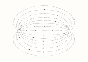
 $b$). The pumped water may be eventually used (after treating) to recharge. The question of relevance here is whether a doublet represents a realistic model for a system of injecting/pumping wells. It is well known (Dagan Reference Dagan1978) that this is authorized when the well radius $r_w$ is much smaller than the well length. Because $r_w \sim {O}(1 - 10 \, \textrm {cm})$, whereas the aquifer thickness is ${O} (1 - 10 \, \textrm {m})$, replacing a well with a line of singularity is a reasonable approximation. As a consequence, the theoretical study of transport in a doublet-type flow becomes of definite interest for applications. The drawback attached to the doublet is the non-uniformity of the flow field, which makes the simulation (and the successive interpretation) of the BTC very complicated. As it will be clarified later on, such a difficulty is tremendously enhanced by the heterogeneity of the aquifer, and this is (partly) the reason for the very limited analytical studies on such a topic.

Figure 1.  $(a)$ Sketch (lateral view) for solute transport generated by an injecting/pumping well-system of radius $r_w$ through a porous formation $\varOmega$ of thickness $D$.
$D$.  $(b)$ Schematic pattern (plan view) of the streamlines, as determined by the spatially variable advective velocity.
The simplest approach to the problem at hand consists of regarding the formation as homogeneous with constant conductivity (a comprehensive overview of the existing analytical solutions can be found in Bruggeman Reference Bruggeman1999). In this case, flow is characterized by streamlines connecting the source with the sink. In particular, Koplik, Redner & Hinch (Reference Koplik, Redner and Hinch1994) have shown that the homogeneous advective field:  $\boldsymbol {u} = u_0 \, \boldsymbol {r} / r^{d-1}$ (where $d=2,3$ is the space-dimensionality) greatly influences transport causing, in particular, huge differences in the mass arrivals along different streamlines and ultimately producing a persistent tailing (modulated by the scaling parameter $u_0$) in the BTC.
However, natural porous formations are, as a rule, heterogeneous, with  $K$ varying in the space by several orders of magnitude (Rubin Reference Rubin2003). Especially in sedimentary formations, heterogeneity manifests as elongated inclusions (lenses) of different permeabilities, which result in a layered pattern. This sets up de facto ‘shortcuts’ connecting the lines through high conductivity zones, which lead to BTCs earlier than in an homogeneous medium (Kurowski et al. Reference Kurowski, Ippolito, Hulin, Koplik and Hinch1994). As a consequence, dispersion is tremendously augmented, as has been detected in a few field-scale transport experiments (Fernández-Garcia, Illangasekare & Rajaram Reference Fernández-Garcia, Illangasekare and Rajaram2004; Ptak, Piepenbrink & Martac Reference Ptak, Piepenbrink and Martac2004).
To account for its erratic variations and the associated uncertainty, it is customary to model the hydraulic conductivity  $K$ as a random field. Thus, the log-conductivity $Y = \ln K$ is regarded as stationary and normal, defined completely by the geometric mean $K_G = \exp (\langle Y \rangle )$ (hereafter, the symbol $\langle \rangle$ will denote the ensemble average operator), variance $\sigma ^2_Y$ and two-point autocorrelation $\rho _Y$. The latter is anisotropic, with the horizontal integral scale, $I$, larger than the vertical one, $I_v$.
Transport in doublet-type flows, where the spatial variability of the hydraulic conductivity is accounted for, has been scarcely studied, its theoretical and practical importance notwithstanding (Kurowski et al. Reference Kurowski, Ippolito, Hulin, Koplik and Hinch1994). With the exception of a few analytical studies (Dagan & Indelman Reference Dagan and Indelman1999; Zech et al. Reference Zech, D'Angelo, Attinger and Fiori2018), to our knowledge, there are only numerical studies simultaneously accounting for the heterogeneity of the aquifer and the non-uniformity of the flow pattern (see Bianchi et al. Reference Bianchi, Zheng, Tick and Gorelick2011, and references therein). However, the strong coupling between the spatially variable hydraulic conductivity and the non-uniformity of the flow poses serious numerical issues. Very dense grids are required in the regions of the flow domain where streamlines converge, which therefore prevent the ability to achieve accurate solutions (especially for highly anisotropic formations). Instead, analytical tools lead to simple (i.e. closed form) solutions. These provide explicit relationships between the input parameters and the model output, therefore giving physical insight into the problem, without resorting to computationally heavy (sometimes prohibitive) numerical simulations.
We aim to investigate the dispersion mechanism in a doublet flow by means of spatial moments. While the dispersion of both passive and reactive solutes in uniform mean flows has been studied extensively in the past (see, e.g. Dagan Reference Dagan1984; Cvetkovic & Dagan Reference Cvetkovic and Dagan1994), much less has been done at the conditions typical of source flows (a review of recent results can be found in Severino, Leveque & Toraldo Reference Severino, Leveque and Toraldo2019) and we are not aware of any theoretical derivation of spatial moments for a doublet-flow configuration. Before proceeding, we wish to clarify the difference between the present study and that of Dagan & Indelman (Reference Dagan and Indelman1999) (similar conclusions can be drawn for the study of Zech et al. Reference Zech, D'Angelo, Attinger and Fiori2018). In these studies, the aim was: (1) to compute the BTC at the sink given the input at the source; and (2) to assess how the heterogeneity of the formation impacts the shape of the BTC. However, such a methodology does not allow for quantification of the dispersion process in the intermediate zone between the two lines (figure 1). In fact, the approach of Dagan & Indelman (Reference Dagan and Indelman1999) relies on the quantification of the probability distribution function of the arrival times of solute particles at the source, and therefore it does not account for the entire history of the spatial dispersion between the release and recovery of the solute. From the standpoint of applications, an important implication concerns the identification of the heterogeneous nature of the conductivity. In fact, unlike the BTC, spatial moments are affected per se by the distribution of the advective velocity between the injecting and pumping lines. As a consequence, the match between the theoretical second-order spatial moments (derived in the present study) and the experimental ones leads to a robust identification of the conductivity field.
The paper is organized as follows: after recalling the general expression of spatial moments, we employ an analytical approximate solution, which ultimately leads to a simple (closed form) expression for the first- and the second-order spatial moments. Then, we discuss the main differences in the dispersion mechanism with transport taking place in other non-uniform flows and we end with our concluding remarks.
2. The transport problem
A passive solute is injected injected in  $\varOmega$ through the sink (figure 1) at a concentration $C_0 \equiv C_0 (\boldsymbol {a})$. We assume that $\varOmega$ is initially solute free. Spatial dispersion can be quantified by means of the first
 \begin{equation} \left \langle R_m (t) \right \rangle = \frac{\vartheta}{M} \int \,\textrm{d} \boldsymbol{a} \left \langle X_m (t; \boldsymbol{a}) \right \rangle C_0 (\boldsymbol{a}) \quad (m = 1,2,3), \end{equation}
and second
 \begin{equation} \left \langle \mathcal{S}_{m,n} (t) \right \rangle = \frac{\vartheta}{M} \int \,\textrm{d} \boldsymbol{a} \left \langle X^\prime_m (t; \boldsymbol{a}) X^\prime_n (t; \boldsymbol{a}) \right \rangle C_0 (\boldsymbol{a}) \quad (m,n = 1,2,3), \end{equation}
order spatial moments (where the constants  $M = \vartheta \int \,\textrm {d} \boldsymbol {a} \, C_0 (\boldsymbol {a})$ and $\vartheta$ are the injected mass and the porosity, respectively). For a pulse of constant concentration $C_0$, moments (2.1)–(2.2) are written as
 \begin{equation} \left \langle R_m (t) \right \rangle \simeq \left \langle X_m (t) \right \rangle, \quad \left \langle \mathcal{S}_{m,n} (t) \right \rangle \simeq \left \langle X^\prime_m (t) X^\prime_n (t) \right \rangle = X_{m,n} (t) \end{equation}
(Dagan Reference Dagan1989). These expressions rely upon two fundamental hypotheses.
(i) Pore scale dispersion $\mathcal {D}$ is neglected. To discuss the feasibility of this approximation, it is instrumental to recall that advection results in the fragmentation of the plume into spots moving quicker/slower than the mean velocity. This produces a concentration gradient between adjacent spots, which ultimately leads to a Fick-type mixing. While this mechanism determines a reduction (dilution) of the local concentration (Fiori & Dagan Reference Fiori and Dagan2000), the matter here is whether $\mathcal {D}$ is also influential on second-order moments (2.2). This can be easily established by comparing the characteristic advection time, $t_a$, relative to the characteristic mixing time, $t_{\mathcal {D}}$. In particular, if $t_a$ is larger than $t_{\mathcal {D}}$, then local dispersion is expected to have a ‘non-negligible’ impact, otherwise it can be ignored. Because typical values of the above characteristic times are such that $t_a / t_{\mathcal {D}} \ll 1$ (see, e.g. Dagan Reference Dagan1989; Rubin Reference Rubin2003), one concludes that pore-scale dispersion can be neglected in the majority of the applications (see also Severino, Santini & Sommella Reference Severino, Santini and Sommella2011; Severino et al. Reference Severino, De Bartolo, Toraldo, Srinivasan and Viswanathan2012a; Zech et al. Reference Zech, D'Angelo, Attinger and Fiori2018);
(ii) Ergodicity, the condition which de facto allows for replacing spatial averages with their statistical counterparts in (2.3a,b), is fulfilled within the present study. More precisely, to invoke the ergodic argument, the thickness
$D$ is required to be much larger than the vertical integral scale $I_v$ (for details, see Dagan Reference Dagan1989, ch. $1.10$). Because $D \sim {O} (1 - 10 \, \textrm {m})$, whereas $I_v \sim {O} (10^{-2} - 1 \, \textrm {m})$ (see, e.g. tables $2.1$–$2.2$ in Rubin Reference Rubin2003), ergodicity is met in most of the real-world situations. As indirect consequence, we can also neglect the effect of the lower/upper boundaries on flow and transport, therefore assuming $\varOmega \cong \mathbb {R}^3$.


Overall, determining the higher-order statistics (typically skewness and kurtosis) would be worthwhile to comprehensively capture the behaviour of the plume. However, logistic as well as economic limitations in the experiments (see, e.g. Fernández-Garcia et al. Reference Fernández-Garcia, Illangasekare and Rajaram2004) do not allow for acquiring the proper dataset needed to compute skewness and kurtosis. For this reason, stochastic tools for the analysis of transport experiments taking place in randomly heterogeneous porous formations generally employ second-order statistics. The usefulness of adopting moments (2.3a,b) to characterize the plume spreading is that they depend directly upon the mean  $\langle \boldsymbol {X} \rangle$ and the fluctuation $\boldsymbol {X}^\prime = \boldsymbol {X} - \langle \boldsymbol {X} \rangle$ of the trajectory $\boldsymbol {X}$ of a fluid particle which, in turn, are determined by the kinematic equation
 \begin{equation} \frac{\textrm{d}}{\textrm{d} t} \boldsymbol{X} = \boldsymbol{u} (\boldsymbol{X}), \quad \boldsymbol{X} (0; \boldsymbol{a}) = \boldsymbol{a}. \end{equation}
Thus, central to quantifying transport is the velocity field  $\boldsymbol {u}$. The latter is not exactly solvable, even for the case of a mean uniform flow (an extensive treatment on this topic can be found in Dagan Reference Dagan1989). In the following, we adopt an approximation for the flow field leading to a simple solution for the transport problem, thereby avoiding heavy (sometimes prohibitive) numerical simulations. Although approximate, the solution for the flow field keeps the salient features of the problem.
2.1. Approximate solution of the velocity field
The system of injecting/pumping wells is replaced by a point-like source/sink (dipole). Such an approximation is valid when the radius  $r_w$ of the wells is much smaller than the distance $\ell$ between them (figure 1 $a$). Because $r_w \sim {O}(1 - 10 \, \mathrm {cm})$, whereas $\ell \sim {O}(1 - 10 \, \mathrm {m})$, this is a reasonable approximation.
We adopt a first-order approximation in the fluctuation  $Y^\prime = Y - \langle Y \rangle$, which has been shown to be quite a robust hypothesis (see, e.g. Firmani, Fiori & Bellin Reference Firmani, Fiori and Bellin2006). Hence, the flow variables (specific energy, flux, etc.) can be expanded in an asymptotic series of $Y^\prime$ and, for each of them, up to the $\sigma ^2_Y$-order, one retains the leading-order term (mean) and the first-order (fluctuation) approximation (an approach similar to the ‘frozen field’ approximation in turbulent flows). Owing to its importance for the transport problem, we focus in the following upon the velocity field. In particular, at the leading order, one has
 \begin{equation} u^{(0)}_m (x_1, x_2) =
\frac{Q}{2 {\rm \pi}n} \begin{cases} \dfrac{4 \ell \left(
\ell^2- 4 x^2_r \right)}{\left( 4 x^2_r + \ell^2 \right)^2-
\left( 4 \ell x_1 \right)^2} & m =1,\\ \dfrac{32 \, \ell \,
x_1 \, x_2}{\left( 4 \ell x_1 \right)^2 - \left( 4 x^2_r +
\ell^2 \right)^2} & \quad m = 2, \end{cases}
\end{equation}
\begin{equation} u^{(0)}_m (x_1, x_2) =
\frac{Q}{2 {\rm \pi}n} \begin{cases} \dfrac{4 \ell \left(
\ell^2- 4 x^2_r \right)}{\left( 4 x^2_r + \ell^2 \right)^2-
\left( 4 \ell x_1 \right)^2} & m =1,\\ \dfrac{32 \, \ell \,
x_1 \, x_2}{\left( 4 \ell x_1 \right)^2 - \left( 4 x^2_r +
\ell^2 \right)^2} & \quad m = 2, \end{cases}
\end{equation}
(Dagan & Indelman Reference Dagan and Indelman1999), where  $x_r = \sqrt {x^2_1+x^2_2}$ is the magnitude of the vectorial position $\boldsymbol {x}_r \equiv (x_1, x_2)$ in the horizontal plane. Thus, at the leading order, the velocity field $\boldsymbol {u}^{(0)}$ is de facto two-dimensional, although transport is still three-dimensional (the fluctuation $\boldsymbol {X}^\prime$ obeys the three-dimensional (2.12)).
To simplify the computational burden, we deal with a formation having the anisotropy ratio  $\lambda = I_v / I$ much less than one. This heterogeneous structure is typical of those (highly anisotropic) formations where the fluctuation $Y^\prime$ along the vertical direction is much larger than that in the horizontal plane (see, e.g. Sudicky Reference Sudicky1986; Zinn & Harvey Reference Zinn and Harvey2003). This authorizes the replacement of the vertical autocorrelation with a ‘white noise’ signal, i.e. $\rho _Y (\boldsymbol {x}) \to \rho _Y (\boldsymbol {x}_r) \, \delta (x_3)$ (for details, see e.g. Fiori, Indelman & Dagan Reference Fiori, Indelman and Dagan1998). This approximation has two fundamental implications.
(i) The fluctuation of the velocity is written as
(2.6)(Dagan & Indelman Reference Dagan and Indelman1999; Indelman & Dagan Reference Indelman and Dagan1999). In fact, adopting (2.6) was found to yield accurate results for the dispersion mechanism already for\begin{equation} \boldsymbol{u}^{(1)} (\boldsymbol{x}) \simeq Y \left( \boldsymbol{x} \right) \boldsymbol{u}^{(0)} (\boldsymbol{x}_r) \end{equation}$\lambda \le 0.2$ (Dagan & Indelman Reference Dagan and Indelman1999). More generally, it has been recently shown that the approximation (2.6) becomes an exact result for $\lambda \to 0$ (stratified formation), even in unsteady non-uniform flows (Severino & Cuomo Reference Severino and Cuomo2020). Because numerous (typically sedimentary) formations are such that $I_v \le I / 10$ (see e.g. tables $2.1$–$2.2$ in Rubin Reference Rubin2003), the above approximation is applicable to many situations of practical interest.(ii) Transport variables become stationary along the vertical and, therefore, they depend only on
$\boldsymbol {x}_r$.


Based on this, we proceed with the computation of moments and, in particular, with the quantification of the dispersion pattern in the zone between the source and the sink.
2.2. Longitudinal dispersion along the central strip delimited by the source/sink
We consider a solute injected at the source (figure 1 $a$). For $t >0$, the plume is advected outwards and it is distorted owing to the $Y$-heterogeneity (figure 1 $b$). It is seen from (2.3a,b) that to characterize the migration of the plume, it suffices to compute the second-order statistics of the trajectory $\boldsymbol {X} \equiv ( X_1, X_2, X_3 )$ of a fluid particle. In particular, because the average velocity is identical to that in an homogeneous medium of conductivity $K_G$, the mean trajectory $\langle \boldsymbol {X} \rangle$ results from (2.4a,b) as follows (chain-rule of derivation):
 \begin{equation} \frac{\textrm{d} \langle X_1 \rangle / \textrm{d} t}{\textrm{d} \langle X_2 \rangle / \textrm{d} t} = \frac{u^{(0)}_1 \left( \langle X_1 \rangle , \langle X_2 \rangle \right)}{u^{(0)}_2 \left( \langle X_1 \rangle , \langle X_2 \rangle \right)} = \frac{\textrm{d} \langle X_1 \rangle}{\textrm{d} \langle X_2 \rangle}, \quad \langle X_3 \rangle = \text{const}. \end{equation}
Then, accounting for the velocity field (2.5) leads to the nonlinear first-order equation,
 \begin{equation} 2 \langle X_1 \rangle \,\textrm{d} \langle X_1 \rangle = \frac{\textrm{d} \langle X_2 \rangle}{\langle X_2 \rangle} ( \langle X_1 \rangle^2 - \langle X_2 \rangle^2 - \bar \ell^{\, 2}) \quad ( \bar \ell = \ell / 2 ), \end{equation}
which is transformed into a linear one after introducing  $\mathcal {Y} = \langle X_1 \rangle ^2$ and $\mathcal {Z} = \ln \langle X_2 \rangle$, i.e.
 \begin{equation} \frac{\textrm{d}}{\textrm{d} \mathcal{Z}} \, \mathcal{Y} = \mathcal{Y} - \exp \left ( 2 \mathcal{Z} \right ) - \bar \ell^{\, 2} \quad \Rightarrow \quad \langle X_1 \rangle^2 = \bar \ell^{\, 2} + C \langle X_2 \rangle - \langle X_2 \rangle^2. \end{equation}
The second part of (2.9) corresponds, for any  $C \in \mathbb {R}$, to a streamline originating at the source. It is easy to show that all the streamlines belong to a bundle of circles (Apollonius), passing by the sink and the source, with centres and radii given by $(0,C)$ and $\sqrt {C^2 + \bar \ell ^{\, 2}}$, respectively. In particular, the trajectories within a tiny strip between the source and the sink are such that $\langle X_2 \rangle \ll \langle X_1 \rangle$ (figure 1 $b$) and, therefore, the longitudinal trajectory $\langle X_1 \rangle \equiv \langle X_1 (t) \rangle$ can be obtained by expanding in Taylor series the right-hand side of (2.4a,b), with $u^{(0)}_1$ given by the first part of (2.5). This leads to
 \begin{equation} \frac{\textrm{d}}{\textrm{d} t} \langle X_1 \rangle = \dfrac{4 \ell \left[ \ell^2- 4 \left ( \langle X_1 \rangle^2 + \langle X_2 \rangle^2 \right) \right]}{\left[ \ell^2 + 4 \left ( \langle X_1 \rangle^2 + \langle X_2 \rangle^2 \right) \right]^2- \left( 4 \ell \langle X_1 \rangle \right)^2} \simeq \frac{Q \bar \ell / ({\rm \pi} n)}{\bar \ell^2 - \langle X_1 \rangle^2 }, \quad \langle X_1 (0) \rangle ={-} \bar \ell. \end{equation}
Solving the above Cauchy problem provides
 \begin{equation} t ( \tilde X ) = \frac{t_c}{3} (2 + 3 \tilde X - \tilde X^3 ), \quad t_c = {\rm \pi}n \frac{\bar \ell^{\, 2}}{Q}, \quad \tilde X = \frac{\langle X_1 \rangle}{\bar \ell}. \end{equation}
Thus, the central normalized trajectory  $\tilde X$ is an increasing function of the time, and it takes time $t(1) = 4/3 \, t_c$ to reach the sink.
We are now in position to compute the trajectory variance  $\langle X^\prime _m X^\prime _n \rangle$, which in turn is related to the fluctuation $\boldsymbol {X}^\prime$ by means of
 \begin{equation} \frac{\textrm{d}}{\textrm{d} t} \, \boldsymbol{X}^\prime = \boldsymbol{u}^{(1)} (\langle \boldsymbol{X} \rangle) + \left( \boldsymbol{X}^\prime \boldsymbol{\cdot} \boldsymbol{\nabla} \right) \boldsymbol{u}^{(0)} \left( \langle \boldsymbol{X} \rangle \right), \quad \boldsymbol{X}^\prime (0) = 0 \end{equation}
(Indelman & Rubin Reference Indelman and Rubin1996). We restrict the analysis to the trajectories along the  $x_1$-direction, because they are of most interest for the spreading mechanism. In fact, the spreading of the plume is advection dominated (see, e.g. Severino, Cvetkovic & Coppola Reference Severino, Cvetkovic and Coppola2005) and therefore dispersion is enhanced along streamlines where the advection velocity is larger. To establish which is the streamline with higher velocity, in the spirit of the employed perturbation approach, one can look at the leading-order approximation $\boldsymbol {u}^{(0)}$ of the flow field. Toward this aim, it is convenient to switch to the new variables $(\phi, \theta )$ that are related to $\boldsymbol {x}_r$ as
 \begin{equation} x_1 = \dfrac{\bar \ell \sinh \phi}{\cosh \phi + \cos \theta}, \quad x_2 = \dfrac{\bar \ell \, \sin \theta}{\cosh \phi + \cos \theta}, \quad \phi \in \mathbb{R}, \quad \theta \in [0, {\rm \pi}[ \end{equation}
(where, in particular,  $\theta$ is the attack angle of the outgoing trajectory). Thus, in the new framework, the magnitude of the velocity results from (2.13a,b) as $|\boldsymbol {u}^{(0)}| \sim \cosh \phi + \cos \theta$, which shows that the streamline exhibiting the largest dispersion is the one along the $x_1$ direction ( $\theta = 0$). For this trajectory, the probability that $X_2 / X_1 \sim {O} ( 1 )$ is quite small, and concurrently the fluctuation $X^\prime _1$ results from (2.12) as
 \begin{equation} \frac{\textrm{d}}{\textrm{d} t} \, X^\prime_1 = u^{(1)}_1 \left( \langle X_1 \rangle, 0 \right) + X^\prime_1 \, \frac{\partial}{\partial \langle X_1 \rangle} \, u^{(0)}_1 \left( \langle X_1 \rangle,0 \right), \quad X^\prime_1 (0) = 0. \end{equation}
The solution of (2.14) is
 \begin{equation} X^\prime_1 (t) = u^{(0)}_1 \left[ \langle X_1 \left( t \right) \rangle,0 \right] \int^t_0 \,\textrm{d} \tau \, \frac{u^{(1)}_1 \left[ \langle X_1 \left( \tau \right) \rangle,0 \right]}{u^{(0)}_1 \left[ \langle X_1 \left( \tau \right) \rangle,0 \right]}, \end{equation}
and thus the variance  $X_{11} (t) = \langle X^{\prime \, 2}_1 (t) \rangle$ along the central streamline reads as
 \begin{equation} X_{11} (t) = u^{(0)}_1 \left[ \langle X_1 \left( t \right) \rangle \right] u^{(0)}_1 \left[ \langle X_1 \left( t \right) \rangle \right] \int^t_0 \int^t_0 \frac{\textrm{d} \tau_1 \, \textrm{d} \tau_2 \, C_{u_{11}} \left( \tau_1, \tau_2 \right)}{u^{(0)}_1 \left[ \langle X_1 \left( \tau_1 \right) \rangle \right] u^{(0)}_1 \left[ \langle X_1 \left( \tau_2 \right) \rangle \right]}, \end{equation}
where, for the sake of brevity, we have replaced  $u^{(0)}_1 [ \langle X_1 ( t ) \rangle,0 ] \to u^{(0)}_1 [ \langle X_1 ( t ) \rangle ]$. In the expression (2.16), $C_{u_{11}} ( t_1, t_2 ) = \langle u^{(1)}_1 [ \langle X_1 ( t_1 ) \rangle ] u^{(1)}_1 [ \langle X_1 ( t_2 ) \rangle ] \rangle$ is the covariance of the velocity field $\boldsymbol {u}$ that is computed by the approximation (2.6) as
 \begin{equation} C_{u_{11}} \left( t_1, t_2 \right) = \sigma^2_Y \, u^{(0)}_1 \left[ \langle X_1 \left( t_1 \right) \rangle \right] u^{(0)}_1 \left[ \langle X_1 \left( t_2 \right) \rangle \right] \rho_Y \left[ \langle X_1 \left( t_1 \right) \rangle, \langle X_1 \left( t_2 \right) \rangle \right]. \end{equation}
Then, substitution into (2.16) leads to
 \begin{equation} X_{11} (t) = \sigma^2_Y u^{(0)}_1 \left[ \langle X_1 \left( t \right) \rangle \right] u^{(0)}_1 \left[ \langle X_1 \left( t \right) \rangle \right] \int^t_0 \int^t_0 \,\textrm{d} \tau_1 \, \textrm{d} \tau_2 \, \rho_Y \left[ \langle X_1 \left( \tau_1 \right) \rangle, \langle X_1 \left( \tau_2 \right) \rangle \right]. \end{equation}
It is worth noting that for a mean uniform flow, i.e.  $u^{(0)}_1 = {\rm const}$, one recovers from (2.18) the same expression (see $(3.10)$ in Dagan Reference Dagan1987) valid for a groundwater flow. For convenience, we switch to the coordinate $\langle X_1 \rangle \equiv \langle X_1 (t) \rangle$ by virtue of the kinematic equation $\textrm {d} \langle X_1 ( t ) \rangle = u^{(0)}_1 [ \langle X_1 ( t ) \rangle ] \,\textrm {d} t$, i.e.
 \begin{equation} X_{11} \left( \langle X_1 \rangle \right) = [ \sigma_Y u^{(0)}_1 (\langle X_1 \rangle)]^2 \int^{\langle X_1 \rangle}_{- \bar \ell} \int^{\langle X_1 \rangle}_{- \bar \ell} \frac{\textrm{d} \alpha \, \textrm{d} \beta \, \rho_Y \left( \alpha - \beta \right)}{u^{(0)}_1 \left( \alpha \right) u^{(0)}_1 \left( \beta \right)}. \end{equation}
Introducing the new variables  $u = \alpha - \beta$ and $v = \beta$ enables one to write
 $$\begin{gather} X_{11} \left( \langle X_1 \rangle \right) = \left [ \sigma_Y u^{(0)}_1 \left( \langle X_1 \rangle \right) \right]^2 \int_0^{\, \bar \ell + \langle X_1 \rangle} \,\textrm{d} u \, \rho_Y (u) \int^{\, \bar \ell + \langle X_1 \rangle}_u \frac{\textrm{d} v}{u^{(0)}_1 \left( v - u - \bar \ell \right)} \nonumber\\ \times \left [ \frac{1}{u^{(0)}_1 \left( v - \bar \ell \right)} + \frac{1}{u^{(0)}_1 \left( v - 2 u - \bar \ell \right)} \right ]. \end{gather}$$
Thus, if the leading-order term  $u^{(0)}_1$ makes it possible to express in closed form the inner quadratures in (2.20), the computation of $X_{11}$ is reduced to the evaluation of a single integral. This latter is then carried out (either analytically or numerically) once the shape of the autocorrelation function $\rho _Y$ is selected. This is just the case for the problem at hand, and the final result reads as
 \begin{equation} X_{11} \left( \langle X_1 \rangle \right) = \left [ \sigma_Y \left (\frac{{\rm \pi} n}{Q \bar \ell} \right) u^{(0)}_1 \left( \langle X_1 \rangle \right) \right]^2 \int_0^{\bar \ell + \langle X_1 \rangle} \,\textrm{d} u \, \rho_Y (u) \, \texttt{P}_5 (u; \langle X_1 \rangle), \end{equation}
where we have set
 $$\begin{gather} \texttt{P}_5 (u; \xi)
={-} \frac{16}{15} \, u^5 + 4 \, \xi u^4 - \frac{2}{3}
( 9 \, \xi^2 - 5 \, \bar \ell^{\, 2} ) u^3 +
\frac{2}{3} ( \xi + \bar \ell \, ) ( 7 \,
\xi^2 - 7 \, \xi \, \bar \ell - 2 \, \bar \ell^{\, 2} \,
) u^2 \nonumber\\ - 2 ( \xi - \bar \ell \,
)^2 ( \xi + \bar \ell \, )^2 u +
\frac{2}{15} ( \xi + \bar \ell \, )^3 ( 3
\, \xi^2 - 9 \, \xi \, \bar \ell + 8 \, \bar \ell^{\, 2} \,) . \end{gather}$$
$$\begin{gather} \texttt{P}_5 (u; \xi)
={-} \frac{16}{15} \, u^5 + 4 \, \xi u^4 - \frac{2}{3}
( 9 \, \xi^2 - 5 \, \bar \ell^{\, 2} ) u^3 +
\frac{2}{3} ( \xi + \bar \ell \, ) ( 7 \,
\xi^2 - 7 \, \xi \, \bar \ell - 2 \, \bar \ell^{\, 2} \,
) u^2 \nonumber\\ - 2 ( \xi - \bar \ell \,
)^2 ( \xi + \bar \ell \, )^2 u +
\frac{2}{15} ( \xi + \bar \ell \, )^3 ( 3
\, \xi^2 - 9 \, \xi \, \bar \ell + 8 \, \bar \ell^{\, 2} \,) . \end{gather}$$
In what follows, we shall discuss the combined effect upon solute dispersion of the heterogeneity of the medium and the flow configuration.
3. Discussion
We wish to illustrate and discuss the results achieved so far. To show, in a simple manner, the main features of the dispersion between the two lines, we regard the fluctuation  $Y^\prime$ as a white noise signal (in analogy with the $\delta$-approximation of the energy spectrum in the theory of homogeneous turbulence). This simplifies tremendously computing the right-hand side of (2.21), and the final result is
 \begin{equation} \frac{X_{11} (\tilde X)}{I \bar \ell \sigma^2_Y} = \frac{2}{15} \frac{1 + \tilde X}{( 1 - \tilde X)^2} \, ( 3 \tilde X^2 - 9 \tilde X + 8 ) \end{equation}
(for convenience, we have taken  $\bar \ell$ as the characteristic length scale). It is seen that $X_{11}$ grows monotonically with the scaled travel distance $\tilde X \in ] - 1, \, 1 [$ (and ultimately with the time $t$). Such a behaviour has a straightforward mechanical explanation by recalling that the variance (3.1) is computed from the outset of the advective velocity field. In fact, close to the release zone, transport is affected by the boundary condition and, concurrently, dispersion is negligible there (it is reminded that the pore-scale dispersion is neglected). Instead, as the travel distance $\tilde X$ increases, the random fluctuations of the velocity field overtake over and over and this justifies the increase of $X_{11}$. Ultimately, the latter becomes unbounded owing to the fact that the velocity at the sink becomes singular. The transitional behaviour from the near (i.e. $\tilde X \simeq -1$) to the far (i.e. $\tilde X \simeq 1$) field is in agreement with Indelman & Dagan (Reference Indelman and Dagan1999) and Severino (Reference Severino2011), who have investigated transport generated by source-type flows.
In figure 2, we have depicted the scaled longitudinal moment  $X_{11} / (I \bar \ell \sigma ^2_Y)$ obtained from (2.21) by considering the exponential $\rho _Y (x) = \exp (- x / I)$, i.e.
 $$\begin{gather} \frac{X_{11} (\tilde X)}{I \bar \ell \sigma^2_Y} = \frac{\mathcal{X}^f (\tilde X) + 4 \tilde I^{\, 2} \exp [ - (\tilde X + 1) / \tilde I ] \mathcal{X}^n (\tilde X) }{(1 - \tilde X)^2 (1 + \tilde X)^2} \quad (\tilde I = I / \bar \ell \,), \end{gather}$$
 $$\begin{gather} \mathcal{X}^f (\xi) = \frac{2}{5} \xi^5 - 2 \tilde I \xi^4 + \frac{4}{3} ( 7 \tilde I^{\, 2} -1 ) \xi^3 - 4 \tilde I ( 9 \tilde I^{\, 2} - 1 ) \xi^2 + 2 ( 48 \tilde I^{\, 4} - 6 \tilde I^{\, 2} + 1 ) \xi \nonumber\\ - \frac{2}{15} ( 960 \tilde I^{\, 5} - 150 \tilde I^{\, 3} + 20 \tilde I^{\, 2} + 15 \tilde I - 8), \end{gather}$$
 $$\begin{gather}\mathcal{X}^n (\xi) = ( \tilde I + 1 ) \xi^2 + 2 ( 2 \tilde I + 1)^2 \xi + 32 \tilde I^{\, 3} + 32 \tilde I^{\, 2} + 11 \tilde I + 1 \end{gather}$$
(a similar result, although much more cumbersome, is obtained by adopting Gaussian  $\rho _Y$) as a function of the distance $\mathcal {R} = \tan [{\rm \pi} (\langle X_1 \rangle +\ell ) / (4 \ell )]$. The utility of the mapping $\langle X_1 \rangle \in ]- \ell, \ell [ \, \, \to \mathcal {R} \in [0, \infty [$ relies upon the fact that, in this way, one can compare with similar results in source-/line-type flows. The most evident feature detected from figure 2 is the increasing dispersion (for a given $\mathcal {R}$) with the smaller $\tilde I$, ultimately reaching the upper bound corresponding to a stratified formation (red line). In fact, to pass through a low conducting inclusion, a fluid particle has to cover a large distance, therefore increasing the correlation length, and hence the velocity covariance $C_{u_{11}}$. As a consequence, the second-order moment $X_{11}$ will also grow owing to its dependence (see (2.16)) upon $C_{u_{11}}$. Such an increase is enhanced by the smallest $\tilde I$ values, because a formation with $I \ll \ell$ implies a longer correlation distance.

Figure 2. The normalized trajectory variance  $X_{11} / (I \bar \ell \sigma ^2_Y)$ for exponential autocorrelation (black lines) as a function of $\mathcal {R}$ and a few values of the non-dimensional integral scale $\tilde I = I / \ell$. For comparison purposes, the trajectory variances for a line (blue) and source (green) flow (Indelman & Dagan Reference Indelman and Dagan1999) have also been included. Finally, the red line depicts (3.1), which corresponds to a stratified formation.
In addition to the computational simplification, the expression (3.1) lends itself as an upper bound for the dispersion mechanism, which in turn can be conveniently accounted for when designing remediation strategies. More precisely, one can select the injecting/pumping flow rate  $Q$ as well as the distance $\ell$ such that dispersion at a certain distance $x^\star \in ]-\ell, \ell [$ is less than a given (regulatory) threshold. It is therefore clear that dealing with a stratified formation, and thus by accounting for the simple expression (3.1), would lead to a conservative estimate.
At the other extreme, line (and a fortiori source) flow constitutes a lower bound for dispersion in a dipole. This is clearly observed in figure 2, where we have also depicted the trajectory variance for a line and source flow, i.e.
 \begin{equation} \frac{X_{11}}{\left( I
\sigma_Y \right)^2} = \begin{cases} \dfrac{2}{3} \,
\mathcal{R} -1 + \dfrac{2}{\mathcal{R}^2} \left[ 1 - \left(
1 + \mathcal{R} \right) \exp \left( - \mathcal{R} \right)
\right] & { ( \textrm{line} ) },\\ \dfrac{2}{5} \,
\mathcal{R} -1 + \dfrac{4}{3 \mathcal{R}} -
\dfrac{8}{\mathcal{R}^4} + \dfrac{4}{\mathcal{R}^2} \left(
1 +\dfrac{2}{\mathcal{R}} + \dfrac{2}{\mathcal{R}^2}
\right) \exp \left( - \mathcal{R} \right) & (
\textrm{source} ), \end{cases}
\end{equation}
\begin{equation} \frac{X_{11}}{\left( I
\sigma_Y \right)^2} = \begin{cases} \dfrac{2}{3} \,
\mathcal{R} -1 + \dfrac{2}{\mathcal{R}^2} \left[ 1 - \left(
1 + \mathcal{R} \right) \exp \left( - \mathcal{R} \right)
\right] & { ( \textrm{line} ) },\\ \dfrac{2}{5} \,
\mathcal{R} -1 + \dfrac{4}{3 \mathcal{R}} -
\dfrac{8}{\mathcal{R}^4} + \dfrac{4}{\mathcal{R}^2} \left(
1 +\dfrac{2}{\mathcal{R}} + \dfrac{2}{\mathcal{R}^2}
\right) \exp \left( - \mathcal{R} \right) & (
\textrm{source} ), \end{cases}
\end{equation}
(Indelman & Dagan Reference Indelman and Dagan1999). The different behaviour of (3.2) as compared with the latter is explained by noting that the velocity, i.e.  $\langle u (\mathcal {R}) \rangle = (2 \mathcal {R})^{-1}$, in a line-type flow and that, i.e. $\langle u (\mathcal {R}) \rangle = (4 \mathcal {R}^2)^{-1}$, in a source-type flow are decreasing with the scaled distance $\mathcal {R}$ (figure 3), whereas in a dipole flow, the velocity
 \begin{equation} \langle u (\mathcal{R}) \rangle = \frac{\left( {\rm \pi}/ 4\right)^2}{\arctan \mathcal{R} \left({\rm \pi}/2 - \arctan \mathcal{R} \right)} \end{equation}
(which is obtained by replacing  $\langle X_1 \rangle \to (4 \ell / {\rm \pi}) \arctan \mathcal {R} - \ell$ in (2.10)) is unbounded at the source (i.e. $\mathcal {R} = 0$) and at the sink (i.e. $\mathcal {R} \to \infty$). As a consequence, the fluctuation of the velocity (which, in the spirit of the perturbation expansion employed in the present study, slightly differs from the mean velocity) is unbounded both at the release and at the recovery of the solute, therefore producing a larger dispersion as compared with that detected in source/line flows.

Figure 3. Non-dimensional (i.e. scaled by  $\bar \ell / t_c$) mean velocity $\langle u \rangle \equiv \langle u (\mathcal {R}) \rangle$ as a function of the normalized distance $\mathcal {R} = \tan [{\rm \pi} (\langle X_1 \rangle +\ell ) / (4 \ell )]$ for a (i) doublet, (ii) single line and (iii) point source type flow.
4. Summary and conclusions
Solute transport in a doublet-type flow through a heterogeneous porous formation has received, in the past, very little attention, its importance in the applications notwithstanding. The main difficulty, which renders this problem very complex, is the coupling between the spatially variable hydraulic conductivity and the strong non-uniformity of the flow field. Even worse, the numerical approach does not seem computationally affordable for highly anisotropic formations of a three-dimensional structure.
In the present study, we have focused on the dispersion process occurring in the strip delimited by the source and the sink (figure 1). An analytical (closed form) expression for the longitudinal spatial moment has been derived. It has been achieved by adopting a few approximations: (i) the log-conductivity is a stationary random field of axisymmetric anisotropy; (ii) a perturbation solution for the flow field is sought; and (iii) pore-scale dispersion is neglected. Dealing with a highly anisotropic formation simplifies considerably the computation of the statistics of the flow field and concurrently the evaluation of the longitudinal spatial moment. The latter is expressed in closed form for any autocorrelation function  $\rho _Y$, which can be straightforwardly evaluated once the shape of $\rho _Y$ is specified. The major difference between transport in a doublet and other similar (typically source and line type) flows is that dispersion in the former is larger than in the latter. This effect arises from the advective velocity (3.6) which, unlike that in source/line flows, is rapidly increasing in the far field owing to the presence there of the singularity.
In addition to the theoretical aspects, expression (2.21) is also useful for the applications. In fact, by taking the limit  $\lambda \to 0$ (stratified formation) provides an upper bound for the dispersion mechanism (figure 2). Thus, it can be adopted as an (conservative) estimate to select the strength $Q$ and the distance $\ell$ of the doublet, when designing remediation strategies. In addition, it is shown that dispersion arising from a single injecting well (Indelman & Dagan Reference Indelman and Dagan1999) constitutes a lower bound for the same mechanism. This is clearly owing to the fact that, unlike the doublet, the advective velocity decays like $\mathcal {R}^{-1}$. Even such a lower bound finds use in the applications concerning the use of chemicals to neutralize dissolved pollutants. In this case, one has to maximize the dispersion to enhance reactions (Di Dato et al. Reference Di Dato, de Barros, Fiori and Bellin2018), and therefore the design accounting for the lower bound certainly provides another conservative estimate of the efficiency of the procedure.
Although the study has focused on dispersion of a passive scalar, it can be extended straightforwardly to reactive solutes along the lines developed by Cvetkovic & Dagan (Reference Cvetkovic and Dagan1994). Even in this case, if one is interested in global quantities (like BTCs or spatial moments), then pore-scale dispersion can be neglected. In fact, the involved reaction equation very often overtakes local mixing (Severino, Dagan & van Duijn Reference Severino, Dagan and van Duijn2000; Severino et al. Reference Severino, Tartakovsky, Srinivasan and Viswanathan2012b). Nevertheless, to assess the efficiency of certain remediation procedures (specifically those relying upon the concentration values), the above global quantities may not result in an appropriate tool. In this case, the computation of the probability distribution function of the concentration value(s) would be preferable and dispersion can not be neglected anymore. Finally, the present study lends itself as a benchmark for validating more involved numerical codes.
Acknowledgments
The constructive comments from three anonymous referees have been deeply appreciated and significantly improved the early version of the manuscript.
Declaration of interests
This manuscript has no data sharing, as all the information is contained in the provided figures. The author reports no conflict of interest.


 Open access