


1. Introduction
Vortex–structure interactions are a canonical fluid mechanics problem that occur in a variety of practical engineering applications. These include aircraft and helicopter flight (Widnall & Wolf Reference Widnall and Wolf1980), marine vessel manoeuvres (Wang & Wan Reference Wang and Wan2020), fluidic energy harvesting (Peterson & Porfiri Reference Peterson and Porfiri2012; Pirnia et al. Reference Pirnia, Hu, Peterson and Erath2017, Reference Pirnia, Browning, Peterson and Erath2018; Pirnia, Peterson & Erath Reference Pirnia, Peterson and Erath2021) and turbo-machinery (Du, Sun & Yang Reference Du, Sun and Yang2016). Additional engineering applications can be found in mitigating acoustic output (Ho & Nosseir Reference Ho and Nosseir1979; Liu et al. Reference Liu, Li, Liu, Hao, Zhang and He2021) and enhancing heat transfer (Cornaro, Fleischer & Goldstein Reference Cornaro, Fleischer and Goldstein1999) from impinging jets. More commonly, biological applications of vortex–cavity interactions arise during filling of the left ventricle through the mitral valve during diastole (Faludi et al. Reference Faludi, Szulik, D'hooge, Herijgers, Rademakers, Pedrizzetti and Voigt2010; Markl, Kilner & Ebbers Reference Markl, Kilner and Ebbers2011; Kheradvar & Falahatpisheh Reference Kheradvar and Falahatpisheh2012; Sotiropoulos, Le & Gilmanov Reference Sotiropoulos, Le and Gilmanov2016; Le et al. Reference Le, Elbaz, Van Der Geest and Sotiropoulos2019; Grünwald et al. Reference Grünwald, Korte, Wilmanns, Winkler, Linden, Herberg, Groß-Hardt, Steinseifer and Neidlin2022), during jellyfish locomotion (Dabiri et al. Reference Dabiri, Colin, Costello and Gharib2005; Gemmell et al. Reference Gemmell, Costello, Colin, Stewart, Dabiri, Tafti and Priya2013; Hoover, Griffith & Miller Reference Hoover, Griffith and Miller2017; Gemmell, Colin & Costello Reference Gemmell, Colin and Costello2018; Costello et al. Reference Costello, Colin, Dabiri, Gemmell, Lucas and Sutherland2021), and even in replacement (i.e. tracheoesophageal) speech (Erath & Hemsing Reference Erath and Hemsing2016).
Many of these biological applications have been investigated extensively. However, historically they have focused on exploring case-specific parameters that are relevant only for the particular problem. For example, prior work has explored left ventricle filling efficiency for a vortex ring injected into a confined domain with normal, semi-oblate, semi-prolate and hemispherical surfaces (Samaee Reference Samaee2019). Even this more fundamental approach to the problem of vortex ring impingement on concave surfaces is still problem-specific as it explores only cardiac-relevant geometries. Similarly, the vortex ring generation and surface geometry are confined in an effort to specifically model left ventricle filling. While providing insight into cardiac fluid mechanics, this types of approach limits application to the more fundamental problem of vortex ring–concave surface interactions – the general problem of interest in this work. To the authors’ knowledge, in fact, only two studies (Jianhua et al. Reference Jianhua, Xiaohai, Dong, Zeqing, Zhihua and Andreopoulos2018; New et al. Reference New, Long, Zang and Shi2020), discussed in detail below, have explored this latter class of interaction.
Commonly investigated in laboratory settings, one of the simplest cases of vortex–surface interactions arises as an axisymmetric vortex ring impinges normally on a flat wall. An axisymmetric vortex ring can be generated by ejecting a slug of fluid through an orifice (Gharib, Rambod & Shariff Reference Gharib, Rambod and Shariff1998), as shown schematically in figure 1. The properties of the ejected vortex (i.e. vortex radius ( $R_{v}$), core radius ( $R_\mathrm {c}$), circulation ( $\varGamma$) and advection velocity ( $U_{a})$ are determined by the piston geometry, i.e. piston diameter ( $d_{t})$, piston velocity ( $U_p$) and piston travel ( $L$). The cylindrical coordinate system shown in figure 1 will be adopted throughout the paper. The coordinates can be non-dimensionalized as $r^* = r/d_t$ and $z^* = z/d_t$, where $d_t$ is the piston tube diameter. Note that $z^* = 0$ corresponds to the exit plane of the vortex tube.

Figure 1. Schematic diagram of variables associated with piston–tube vortex ring generation.
As a vortex ring approaches an infinite wall, it induces a radial flow on the surface. This gives rise to a pressure gradient that decreases radially from the centreline stagnation point to the ring radius, and then increases due to the expanding geometry bounded by the vortex core and the wall (Boldes & Ferreri Reference Boldes and Ferreri1973; Lim, Nickels & Chong Reference Lim, Nickels and Chong1991; Cheng, Lou & Luo Reference Cheng, Lou and Luo2010). As the vortex ring moves closer to the wall, the ring diameter increases, the axial velocity decreases, the core radius decreases, and due to the resultant vortex stretching, the peak vorticity increases by as much as  $50\,\%$ (Boldes & Ferreri Reference Boldes and Ferreri1973; Lim et al. Reference Lim, Nickels and Chong1991; Fabris, Liepmann & Marcus Reference Fabris, Liepmann and Marcus1996; Cheng et al. Reference Cheng, Lou and Luo2010). If a no-slip condition exists at the wall, then a boundary layer with opposite sign vorticity will be generated. Due to confinement of the boundary layer by the vortex ring, an adverse pressure gradient develops, driving boundary layer growth.
The physics of the interaction is determined by the Reynolds number, which can be expressed in terms of the circulation of the vortex ring  $\varGamma$ as ${{Re}}_{\varGamma} =\varGamma /\nu$, where $\nu$ is the kinematic viscosity (Walker et al. Reference Walker, Smith, Cerra and Doligalski1987). It may alternatively be expressed in terms of the advection velocity, ${{Re}}_v= 0.5U_{a} R_{v}/\nu$ (Saffman Reference Saffman1970). At low Reynolds numbers, the wall-bounded vorticity layer does not separate from the surface (Cerra & Smith Reference Cerra and Smith1983; Peace & Riley Reference Peace and Riley1983; Walker et al. Reference Walker, Smith, Cerra and Doligalski1987). With increasing Reynolds number, the vorticity layer separates from the wall due to the adverse pressure gradient, creating a secondary vortex ring (SVR) that orbits the primary vortex ring (PVR). Mutual induction between the primary and secondary rings causes rebound in the trajectory of the primary ring. A tertiary vortex ring (TVR) may also form (Boldes & Ferreri Reference Boldes and Ferreri1973; Cerra & Smith Reference Cerra and Smith1983; Walker et al. Reference Walker, Smith, Cerra and Doligalski1987; Verzicco & Orlandi Reference Verzicco and Orlandi1996; Rockwell Reference Rockwell1998; Cheng et al. Reference Cheng, Lou and Luo2010; Bourguet, Karniadakis & Triantafyllou Reference Bourguet, Karniadakis and Triantafyllou2011). For Reynolds numbers ${{Re}}_v>2400$, the secondary and tertiary vortex rings can merge, ultimately advecting away from the wall (Harvey & Perry Reference Harvey and Perry1971; Cerra & Smith Reference Cerra and Smith1983; Shariff & Leonard Reference Shariff and Leonard1992).
The azimuthal coherency of the secondary and tertiary vortex rings decreases as the Reynolds number of the primary vortex ring increases (Cerra & Smith Reference Cerra and Smith1983; Walker et al. Reference Walker, Smith, Cerra and Doligalski1987; Cheng et al. Reference Cheng, Lou and Luo2010; Ren & Lu Reference Ren and Lu2015). Azimuthal waviness in the secondary ring arises from either instability in the primary ring, or instability caused by compression of the secondary vortex ring as it orbits the primary ring (Verzicco & Orlandi Reference Verzicco and Orlandi1996). Depending on the Reynolds number of the primary vortex ring, two different classes of secondary ring waviness may arise, namely, loop or kink structures (Walker et al. Reference Walker, Smith, Cerra and Doligalski1987).
In vortex ring–inclined plate (i.e. angles other than  $90^{\circ }$) interactions, significantly different dynamics arise (Verzicco & Orlandi Reference Verzicco and Orlandi1994; New, Shi & Zang Reference New, Shi and Zang2016). The wall-bounded vortex first separates beneath the near end (closest to the wall) of the primary ring. As the near end of the ring contacts the wall, the boundary layer grows rapidly, the core of the primary vortex ring is compressed in the region about the impact point, and intense stretching of the ring at the impact point occurs (Lim Reference Lim1989; Verzicco & Orlandi Reference Verzicco and Orlandi1994). In contrast, the far end of the ring (farthest from the wall) is not affected and thus remains largely intact. The vortex stretching in the near end intensifies the vorticity of the core and therefore creates a non-uniform vorticity distribution along the vortex ring core. This generates bi-helical vortex lines that are displaced continuously and compressed towards the far end of the ring (Lim Reference Lim1989; New et al. Reference New, Shi and Zang2016). The vorticity layer separates from the wall and rolls up as a secondary vortex ring. Cross-sign interactions between the primary and secondary structures lead to rapid localized annihilation of the primary ring at the near end. Conversely, the far end of the primary ring is not subject to high stretching. Consequently, the secondary vorticity that is produced forms a vortex loop structure that folds over on itself and moves away from the wall (Verzicco & Orlandi Reference Verzicco and Orlandi1994, Reference Verzicco and Orlandi1996; Couch & Krueger Reference Couch and Krueger2011).
When vortex rings interact with non-planar surfaces (e.g. cylinders, foils, fins, corners of cavities; Hrynuk, Van & Bohl Reference Hrynuk, Van and Bohl2012; An, Fultz & Hassanipour Reference An, Fultz and Hassanipour2014; Cheng, Lou & Lim Reference Cheng, Lou and Lim2014; Morris & Williamson Reference Morris and Williamson2016; Li & Bruecker Reference Li and Bruecker2018), they can exhibit very different flow behaviours. Unfortunately, there are very few studies that extend the generalized investigation of plane surface interactions to concave surfaces. To the authors’ knowledge, there are only two prior works (Jianhua et al. Reference Jianhua, Xiaohai, Dong, Zeqing, Zhihua and Andreopoulos2018; New et al. Reference New, Long, Zang and Shi2020), although neither of them specifically considers three-dimensional vortex ring impingement on axisymmetric three-dimensional concave cavities, which is the problem of interest in this study.
Nevertheless, Jianhua et al. (Reference Jianhua, Xiaohai, Dong, Zeqing, Zhihua and Andreopoulos2018) numerically simulated a vortex dipole interacting with two-dimensional concave hemispherical cavities. The simulations identified the key physics produced by the interaction, namely, edge vorticity generated on the cavity lip, separation of vortices from the induced wall boundary layer, and the mutual interaction of secondary and primary vortices. A strong link was shown to exist between  $\gamma$ and the evolution of the vorticity field. In a related study, New et al. (Reference New, Long, Zang and Shi2020) considered three-dimensional vortex ring interactions with a V-shaped cavity for different included valley angles ( $\theta$). Their experimental analysis identified that upon impacting the cavity in the valley plane, the primary vortex rings’ core size reduced and moved towards the valley. Secondary and tertiary vortex rings were generated, and ultimately rotated around the primary vortex ring. The entire interaction occurred more rapidly than in the flat plate case, and occurred over decreasingly shorter times with decreasing valley angles. During the interactions the rate of vorticity diffusion in the primary ring increased with valley angle. Although this work has provided insight into how concave geometries influence vortex ring–surface interactions, surprisingly there remains a knowledge gap that details the influence of surface curvature on the most basic scenario of confined axisymmetric vortex ring–surface interactions.
To this end, the work presented herein aims to fundamentally explore vortex–concave cavity interactions, including both surface and edge effects, arising from axisymmetric vortex rings impinging on hemispherical cavities of varying radius. Emphasis is placed on identifying the different flow regimes and behaviours that arise as a function of radius of surface curvature. This is achieved by employing both flow visualization and two-dimensional particle image velocimetry (PIV) to explore the kinematics of the interactions. The work is organized as follows. The flow facility and analysis methods are described in § 2. The results are presented in § 3, where two distinct regimes of interaction are identified and discussed, and § 4 includes the discussion. Finally, § 5 presents the conclusions.
2. Experimental facility and methods
2.1. Experimental facility
Vortex–cavity interactions were investigated in a  $91\,\%$ clear Diamant glass water tank measuring $40.00\,\mathrm {cm}$ ( $15.75\,\mathrm {in}$) long, by $40.00\,\mathrm {cm}$ ( $15.75\,\mathrm {in}$) wide, by $40.00\,\mathrm {cm}$ ( $15.75\,\mathrm {in}$) high. The tank size was selected to minimize interactions with the wall, producing a vortex decay rate $\beta$ less than $10$ (Stewart et al. Reference Stewart, Niebel, Jung and Vlachos2012). Vortex rings were generated using a custom-designed piston–tube arrangement, as shown in figure 2. The piston was housed inside a clear acrylic tube that was $30.50\,\mathrm {mm}$ ( $12.0\,\mathrm {in}$) long. It had outer diameter $50.80\,\mathrm {mm}$ ( $2.00\,\mathrm {in}$) and smooth inner diameter $38.10\,\mathrm {mm}$ ( $1.50\,\mathrm {in}$), with tolerance ${\pm }0.0025\,\mathrm {mm}$ ( $0.001\,\mathrm {in}$). The exit of the cylinder was chamfered externally at $20^{\circ }$ to promote vorticity detachment (Syed & Sung Reference Syed and Sung2009).

Figure 2. Schematic diagram of the experimental facility, including the PIV system.
The piston body consisted of a disk with a circumferential O-ring to maintain a watertight connection and facilitate smooth motion inside the acrylic tube. The piston was attached via a connecting rod to a  $12\,\mathrm {V}$ light-duty linear actuator (Concentric (Pololu), LACT12P-12 V-05) with a 5 : 1 gear ratio. A Jrk G2 24v13 USB motor controller with feedback was paired with an Arduino Uno to control the speed and position of the actuator. A widely-used impulse velocity waveform was chosen due to the ability to compare the generated vortex ring properties with existing data that utilize similar waveforms (Lim Reference Lim1989; Gharib et al. Reference Gharib, Rambod and Shariff1998; Rosenfeld, Rambod & Gharib Reference Rosenfeld, Rambod and Gharib1998; Shusser et al. Reference Shusser, Rosenfeld, Dabiri and Gharib2006; Peterson & Porfiri Reference Peterson and Porfiri2012). The time history of the piston velocity profile is shown in figure 3. The stroke length $L$ of the piston was $101.60\,\mathrm {mm}$ ( $4.00\,\mathrm {in}$), which gives a formation number ( $F$) of $L/d_{t} = 2.67$ (Gharib et al. Reference Gharib, Rambod and Shariff1998). The stroke ratio and piston velocity produced a vortex ring with radius $R_{V} \approx 25.4\,\mathrm {mm}$ at Reynolds number ${{Re}}_{\varGamma } = \varGamma /\nu = 1450$. The distribution of the vorticity along a line bisecting the core of the PVR is provided in supplementary figure 1 (available at https://doi.org/10.1017/jfm.2023.501) for each of the cases discussed below.

Figure 3. Relationship between piston velocity and time.
The contact surfaces were produced by attaching clear plastic hemispheres of varying diameter ( $d_h$) to the hemisphere mount on the bottom of the tank. The thickness of the hemisphere walls was $3.50\,\mathrm {mm}$. Hemisphere radii $R_{H} = d_{h}/2= 38.10\,\mathrm {mm}$ ( $1.50\,\mathrm {in}$), $50.80\,\mathrm {mm}$ ( $2.00\,\mathrm {in}$), $63.50\,\mathrm {mm}$ ( $2.50\,\mathrm {in}$), $76.20\,\mathrm {mm}$ ( $3.00\,\mathrm {in}$), $101.60\,\mathrm {mm}$ ( $4.00\,\mathrm {in}$) and $\infty$ (a flat pate), were employed. The ratio of the vortex ring to hemisphere cavity radius was expressed as $\gamma = R_V/R_H$. The vortex ring radius was constant, with $R_V \approx 25.40\,\mathrm {mm}$. This produced values $\gamma \approx 0, 1/4, 1/3, 2/5, 1/2, 2/3$ for decreasing contact surface radii. The range of values for $\gamma$ was chosen based on the limiting case of a flat plate ( $\gamma \approx 0$) and the scenario for which the vortex ring propagated around, rather than interacting with, the hemisphere ( $\gamma > 2/3$). The hemispheres were fabricated using precision casting under controlled temperature and pressure, thereby providing excellent optical clarity with minimal distortion.
2.2. Experimental methods
Flow visualization was performed to obtain insight into the vortex–hemisphere interactions. Blue food dye was mixed with whole milk and  $70\,\%$ isopropyl alcohol. The milk impeded diffusion of the dye into the water, while the alcohol ensured that the mixture was neutrally buoyant. The final solution was $30\,\%$ food dye, $25\,\%$ whole milk, $20\,\%$ alcohol and $25\,\%$ tap water, by weight. Flow visualization was recorded with a motion pro X3 plus high-speed camera with $4\,\mathrm {GB}$ of internal memory storage, and monochromatic pixel resolution $1280\,\mathrm {pixel} \times 1080\,\mathrm {pixel}$. Flow visualization data were acquired at $10.00\,\mathrm {Hz}$ for $60.00\,\mathrm {s}$. IDT Motion Studio software version 2.15.01.00 was used for video capture. The contrast of the images was adjusted manually to minimize the background intensity.
Planar laser-induced fluorescence (PLIF) was also employed for visualization. A  $532\,\mathrm {nm}$, $100\,\mathrm {mW}$ Aixiz laser was used to excite a fluorescein (disodium salt) solution. The same camera, lens and software set-up as discussed above was used to capture the images at a $10\,\mathrm {Hz}$ frame rate. Two visualization conditions were employed. (1) A syringe and tube arrangement was used to carefully flood the inside of the vortex tube with the prepared dye solution, thereby seeding the vortex ring. (2) A syringe was used to carefully deposit a layer of fluorescein solution on the surface of the hemisphere, thereby enabling visualization of the secondary vorticity induced during vortex impingement on the surface. Again, the contrast of the images was adjusted manually to minimize the background intensity.
Velocity field measurements were performed using two-dimensional PIV. The water in the tank was seeded with Cospheric fluorescent red polyethylene microspheres ( $995\,{\rm kg}\,{\rm m}^{-3}$) with diameter $212\unicode{x2013}250\,\mathrm {\mu }\mathrm {m}$. Because the particles are naturally hydrophobic, a solution was created by adding Tween $20$ Biocompatible surfactant. The resultant particles had peak excitation wavelength $607\,\mathrm {nm}$, and peak emission wavelength $575\,\mathrm {nm}$. The particles were illuminated with a Litron Nano $532\,\mathrm {nm}$ Nd:YAG laser with $50\,\mathrm {mJ}\,\mathrm {pulse}^{-1}$. A light sheet was produced such that it bisected the axis of the vortex tube, as shown in figure 2. A LaVision sCMOS camera ( $2560\,\mathrm {pixel} \times 2160\,\mathrm {pixel})$ was oriented perpendicular to the light sheet at distance $711.2\,\mathrm {mm}$ ( $28.00\,\mathrm {in}$). A NIKKOR $70\,\mathrm {mm}$ lens provided a field of view $210\,\mathrm {mm} \times 180\,\mathrm {mm}$. A $550\,\mathrm {nm}$ long-pass filter was placed over the camera lens when acquiring images to improve near-wall resolution by eliminating laser light reflections. The DaVis PIV self-calibration technique, which implements image dewarping, was used to calibrate the images while also accounting for image distortion due to mismatched indices of refraction. This was performed by imaging a grid of known spacing at the data plane (inside the hemisphere surface) and then correcting the image distortion using the DaVis image dewarping function. Thirty-five image pairs with $dt = 0.013\,\mathrm {s}$ were acquired at $1\,\mathrm {s}$ intervals throughout the interaction, which corresponded to $0.00 \leq t^* \leq 22.67$, where time is non-dimensionalized as $t^* = tU_{p}/d_{t}$.
All velocity fields were interrogated and processed using DaVis 8.2.2 image processing software from LaVision on a  $2\times$ quad-core XEON processor computer with $12\,\mathrm {GB}$ of RAM. The vector fields were computed using recursive $64\,\mathrm {pixel} \times 64\,\mathrm {pixel}$ and $32\,\mathrm {pixel} \times 32\,\mathrm {pixel}$ interrogation windows with $50\,\%$ overlap. This resulted in a vector spacing of $1.30\,\mathrm {mm}$. No post-processing of the vector fields was performed.
The PIV fields were analysed, and the vorticity fields, positions of the initial and induced vortex rings, and corresponding circulation of each ring were computed in time. For each case (i.e. value of  $\gamma$), the vorticity plots were non-dimensionalized as $\omega ^* = \omega / (\varGamma _{max,PVR}/{\rm \pi} R_c^2 )$, where $\varGamma _{max,PVR}$ is the peak circulation of the primary vortex ring (PVR) for each case, which was computed after vortex ring pinch-off and prior to interaction with the surface. For all cases, this occurred at $t^* = 2.67$.
The locations of the cores for each ring were determined by computing and tracking the maximum Q-criterion (Kolář Reference Kolář2007; Holmén Reference Holmén2012) in time. Supplementary figure 2 shows an example of the Q-criterion contours and associated profiles at one instance in time. Due to the temporal dependence of the secondary vortex ring (SVR) and tertiary vortex ring (TVR) formation, the inceptions of the SVRs and TVRs were identified when there was a clear separation of the boundary layer into a coherent structure as indicated by the emergence of closed Q-criterion contours. The locations were tracked until either the time of acquisition ended or multiple peaks in the Q-criterion value emerged in the same domains that had exhibited a clear peak previously, indicative of vortex reconnection and/or breakdown.
The instantaneous circulation of each ring was computed as the area integral of the vorticity over the bounds of the largest closed contour of the Q-criterion, where the circulation was reported as the magnitude averaged over both cores. The corresponding value of the cross-sectional area of the vortex core was then computed and expressed as  ${\rm \pi} R_c^2$, where $R_c$ is the equivalent core radius that yields the same cross-sectional area as the actual core. The mean values of the maximum circulation and core area of the PVR across all cases were found to be $821\times 10^{-6}\,{\rm m}^2\,{\rm s}^{-1} \pm 5\,\%$ and $380\times 10^{-6}\,\mathrm {m}^2\pm 5\,\%$, respectively.
Finally, the temporal behaviour of the primary and induced vortices was determined by computing the non-dimensionalized circulation, which was expressed as  $\varGamma ^* = \varGamma / \varGamma _{max,PVR}$.
2.3. Velocity field uncertainty
Uncertainty in the PIV velocity field data was quantified by considering error due to the ability of the tracer particles to follow the flow, as well as errors arising due to computation of the velocity fields. The tracer particle diameter ( $212\unicode{x2013}250\,\mathrm {\mu }\mathrm {m}$) was large enough that Brownian motion was negligible. Additionally, the particle Stokes number was computed to be less than $0.1$, allowing error due to particle inertia to be neglected (Dring Reference Dring1982). The dominant contribution of the relative error in the tracer particles arises due to the sedimentation velocity, which was computed to be ${\pm }0.14\,\%$ based on the average advection velocity of the PVR at $t^* = 2.67$ ( $0.023\,\mathrm {m}\,\mathrm {s}^{-1}$). The error in the estimation of the velocity from the PIV measurements arises from uncertainty in detecting the particle displacements, with modern algorithms (e.g. as found in DaVis software) producing ${\sim }0.05\unicode{x2013}0.10\,\mathrm {pixel}$ accuracy (Sciacchitano & Wieneke Reference Sciacchitano and Wieneke2016). The timing accuracy of the LaVision programmable timing unit was $100\,\mathrm {ns}$. For observed particle displacement of approximately $6\,\mathrm {pixel}$ in the regions of interest of the flow, and the image pair timing of $dt = 0.013\,\mathrm {s}$ that yields this displacement, the relative uncertainty of the velocity estimation was ${\pm }1.67\,\%$. The total relative velocity uncertainty for the PIV acquisitions was then ${\pm }1.68\,\%$.
The largest source of uncertainty occurred due to the ensemble-averaged velocity fields, where instabilities in the flow interactions sometimes produced slightly variations in the velocity field. To counter this effect,  $70$ velocity fields were averaged for each instance in time. This value was chosen by minimizing the root-mean-square error between an increasing number of averaged velocity fields and a very large sample size ( $365$). The number of averaged velocity fields ( $70$) was chosen by identifying the point at which the error ultimately asymptoted to a constant value of approximately $0.026\,\%$.
3. Results and discussion
3.1. Flat plate interactions ( $\gamma = 0$)

To validate the experimental facility, the widely studied case of a vortex ring impinging on a flat plate was first considered. The interaction exhibits the same physics that has been reported previously in the literature (Cerra & Smith Reference Cerra and Smith1983; Walker et al. Reference Walker, Smith, Cerra and Doligalski1987; Verzicco & Orlandi Reference Verzicco and Orlandi1994, Reference Verzicco and Orlandi1996; Fabris et al. Reference Fabris, Liepmann and Marcus1996), which can be determined by comparing figures 4 and 5 with the literature. Figure 4 presents PIV vorticity plots with velocity vectors overlaid at six instances in time throughout the interaction (see supplementary movie 1 for the entire interaction). A relative velocity vector length of  $0.5\,\mathrm {mm}\,\mathrm {s}^{-1}$ is shown in the top right corner of each plot. The areas of negative and positive vorticity are indicated by blue and red, respectively. Note that the vorticity scale for figures 4(a–c) is different than for figures 4(d–f) – this is to more clearly visualize the interactions. In addition, the centres of the primary, secondary and tertiary vortex rings, as identified previously by computing the Q-criterion, are represented as circles, diamonds and squares, respectively. Figure 5 presents the trajectories of the primary, secondary and tertiary vortex ring cores. The temporal progression is colour-coded according to increasing time from blue to red.

Figure 4. Vorticity contours with velocity vectors overlaid for  $\gamma = 0$ at six different instances in time: (a) $t^* = 0.00$, (b) $t^* = 5.33$, (c) $t^* = 8.67$, (d) $t^* = 12.00$, (e) $t^* =18.67$, and (f) $t^* = 21.33$. A reference vector $0.5\,\mathrm {mm}\,\mathrm {s}^{-1}$ is shown in each plot. The PVR (circle), SVR (diamond) and TVR (square) cores are labelled.

Figure 5. Positions of the primary (circle), secondary (diamond) and tertiary (square) vortex ring cores. Non-dimensional time is indicated by the colours of the symbols.
When the PVR approaches the flat wall, opposite sign vorticity is induced on the wall (figure 4b) and the diameter of the ring increases. Figure 5 shows that the initial diameter of the PVR is  $r^* = r/d_{t} \approx 1.33$. As it approaches the wall, the diameter increases to $r^* \approx 1.62$. The wall-bounded vorticity sheet separates from the wall along the outer periphery of the PVR (figure 4c) due to the adverse pressure gradient (Doligalski, Smith & Walker Reference Doligalski, Smith and Walker1994). The separated vorticity rolls up and generates an SVR, as seen in figure 4(c). Due to the mutual interaction between the PVR and SVR, the PVR experiences a rebound from the wall and reversal of motion (back towards the wall, i.e. a second impact), as can be seen in the inset of figure 5. A TVR is generated at the wall after the second impact of the PVR on the wall at $t^* \approx 12$ (figure 4d). This TVR rotates around the PVR due to mutual induction (figures 4d,e), with the SVR and TVR eventually merging (figure 4e; Cerretelli & Williamson Reference Cerretelli and Williamson2003). After the second impact with the wall, the diameter of the PVR continues to increase, with the largest value reaching $r^* \approx 2.41$ (figure 5). The continuous growth of the PVR diameter results in the generation and rotation of the TVR farther away from the centre line. The features observed in the vortex ring–flat plate interaction in the current facility are the same as those identified in the literature for this orientation (Cerra & Smith Reference Cerra and Smith1983; Verzicco & Orlandi Reference Verzicco and Orlandi1994, Reference Verzicco and Orlandi1996; Fabris et al. Reference Fabris, Liepmann and Marcus1996).
Figure 6 presents the non-dimensional circulation  $\varGamma ^*$ of the primary, secondary and tertiary vortex rings as a function of non-dimensionalized time $t^*$. The dashed vertical line indicates the time when the PVR first impacts the flat plate. Figure 6 demonstrates behaviour that is similar to prior studies (Orlandi & Verzicco Reference Orlandi and Verzicco1993; Fabris et al. Reference Fabris, Liepmann and Marcus1996). The circulation of the PVR increases slightly as it approaches the flat wall due to the vortex stretching. After collision, the circulation of the PVR decreases dramatically due to interactions with the SVR and TVR, as well as diffusion at the boundary. The SVR and TVR exhibit an initial increase in circulation before decaying.

Figure 6. Circulation of the PVR (circle), SVR (diamond) and TVR (square) as functions of time. All values are non-dimensionalized by the maximum circulation of the PVR. The dashed vertical line indicates the time at which the PVR impacts the plate.
3.2. Surface vorticity interactions ($\gamma = 1/4$, 1/3, and 2/5)

Figure 7 presents PIV vorticity plots with velocity vectors overlaid of the vortex ring impinging on concave hemispheres with  $\gamma = 1/4, 1/3, 2/5$. The entire interaction can be seen in supplementary movie 2. The relative velocity vector length $0.50\,\mathrm {mm}\,\mathrm {s}^{-1}$ is shown in the top right corner of each plot in figure 7(iii). The left (i), centre (ii) and right (iii) columns correspond to decreasing hemisphere radius, resulting in $\gamma = 1/4$, $1/3, 2/5$, respectively. The descending rows indicate increasing time, with (a–f) spanning $t^* = 0.00$ to $t^*=21.33$. Again, the centres of the primary, secondary and tertiary vortex rings, as identified by computing the Q-criterion, are represented as circles, diamonds and squares, respectively. Figure 8 presents the core position of the primary, secondary and tertiary vortex cores as functions of time. The insets of figure 8 present a zoomed-in view of the PVR trajectory. Figures 9(a–f) present PLIF flow visualization of the secondary and tertiary vortices at six instances in time, with columns (i), (ii) and (iii) corresponding to varying hemisphere radii such that $\gamma = 1/4$, $1/3$ and $2/5$, respectively. These data are included to provide a clearer visualization of the instantaneous SVR and TVR formation, as opposed to the phase-averaged representation presented in the PIV plots of figure 7. The full interaction can be found in supplementary movie 3.

Figure 7. Vorticity contours with velocity vectors overlaid, interacting with concave hemispheres of (i)  $\gamma = 1/4$, (ii) $\gamma = 1/3$, (iii) $\gamma = 2/5$, at six different instances in time: (a) $t^* = 0.00$, (b) $t^* = 5.33$, (c) $t^* = 8.67$, (d) $t^* = 12.00$, (e) $t^* =18.67$, and (f) $t^* = 21.33$. The PVR (circle), SVR (diamond) and TVR (square) cores are labelled.

Figure 8. Positions of the PVR (circle), SVR (diamond) and TVR (square) cores. Non-dimensional time is indicated by the colours of the symbols.

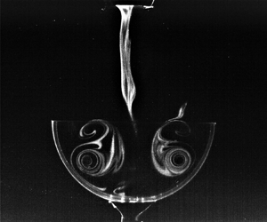
Figure 9. PLIF visualization of the SVR development following collision of a PVR with  ${{Re}}_\varGamma = 1450$ and $F = 2.67$ interacting with (i) $\gamma = 1/4$, (ii) $\gamma = 1/3$, (iii) $\gamma = 2/5$, at six different instances in time: (a) $t^* = 0.00$, (b) $t^* = 5.33$, (c) $t^* = 8.67$, (d) $t^* = 12.00$, (e) $t^* =18.67$, and (f) $t^* = 21.33$.
When the PVR approaches the hemisphere, a very small amount of edge vorticity is generated at the lip (figure 7a) due to separation of the velocity induced by the PVR. Because the hemisphere radius is at least twice the vortex ring radius for each of these cases, this vorticity does not influence the primary ring significantly as it advects towards the bottom of the hemisphere. Preceding contact with the hemisphere, a thin sheet of opposite sign vorticity is generated on the inner surface of the concave wall (figure 7b), as occurs in previously investigated vortex dipole–concave surface interactions (Jianhua et al. Reference Jianhua, Xiaohai, Dong, Zeqing, Zhihua and Andreopoulos2018) and vortex ring–wall interactions (Cerra & Smith Reference Cerra and Smith1983; Verzicco & Orlandi Reference Verzicco and Orlandi1994). As the vortex ring continues to approach the wall, the primary ring diameter increases (figure 7) and the core radius decreases (see figures 7b,c). From figure 8, it can be seen that the initial diameter of the vortex ring for all three cases is  $r^* \approx 1.33$. As the ring comes into contact with the wall, the diameter begins to increase but is ultimately constrained by the geometry. Consequently, the maximum diameter of the vortex ring reaches decreasing values $r^* \approx 2.13$, $1.96$ and $1.87$ for $\gamma =1/4$, $1/3$ and $2/5$, respectively (see figure 8). Note that all of these values are lower than the maximum diameter observed for the flat wall ( $\gamma = 0$) case, which was $r^* = 2.41$ (see figure 5).
An SVR is generated due to separation of the induced vortex sheet (figures 7(b,c) and 9(b,c)), after which mutual induction between the PVR and SVR causes the secondary ring to orbit the primary ring (figures 7(c) and 9(c)), as occurs during the flat plate interactions. This produces a rebound in the PVR trajectory after which it moves back towards the wall and experiences a second impact (see insets of figure 8). This is clearly visible in supplementary movie 4. Due to the second impact, a TVR is generated from the wall-bounded vorticity (figures 7(c) and 9(e)). The TVR also rotates around the PVR due to mutual induction (figure 8). At the conclusion of the interaction, the core of the PVR moves towards the centreline of the hemisphere (see insets of figure 8). This is similar to prior work showing that vortex rings move towards the valley of a V-shaped wall following impact (New et al. Reference New, Long, Zang and Shi2020).
Because the diameter of the PVR is constrained by the geometry (compare figures 7(i–iii) with figure 4), the diameters of the SVR and TVR are also smaller. Subsequently, as the secondary and tertiary rings orbit the primary ring, portions of them appear to experience a head-on collision, as seen in figures 7(d,e) and 9(d,e). To elucidate the physics of this behaviour, flow visualization of the SVR and TVR kinematics for each of the ratios of  $\gamma$ was performed from a front view (figure 10) and an oblique view ( $30^\circ$ from the PVR advection axis; figure 11) by seeding the hemisphere surface with dye. In figure 11, only the first three instances are presented for brevity. The entire interactions can be seen in supplementary movies 5 and 6. Again, the columns differentiate the values of $\gamma$, while the rows indicate the temporal evolution. Note that for all cases, the PVR was stable with no instabilities observed before impact (not shown for brevity) with a constant ring diameter (see figure 8). After impact, an SVR is produced, which is initially symmetric (see figures 10(a) and 11(a)). However, once the SVR starts rotating around the primary ring, the confinement of the ring leads to azimuthal instabilities, evidenced by the emergence of a loop-like instability (figures 11b,c). Each loop has two extremities: a lower end, which corresponds to the minimal ring diameter, and an upper end, which corresponds to the maximum diameter of the deformed ring (figure 10c). The lower ends of the loop are positioned closer to the centre of the PVR, whereas the upper ends are farther away. The proximity of the lower ends of the SVR to the primary ring results in the lower ends orbiting the primary ring in a tighter arc, ultimately being ingested into the the core of the PVR (see figures 10d,e). The relatively longer distance from the upper ends of the secondary vortex loops to the primary ring results in a lower induced velocity. Consequently, the upper ends transcribe a longer arc. As a result, the opposing sides of the upper ends of the secondary vortex loops, now oriented transversely, experience a head-on collision as they orbit around the primary ring (figures 7(d,e), 9(d,e) and 10(d,e)). The subsequent mutual induction between the colliding upper ends moves the looped regions up and away from the hemisphere surface (figures 7(e,f), 9(e,f) and 10(e,f)). The same interaction appears to also happen with the TVR, but the interaction is much weaker. As the upper ends of the SVR and TVR move away from the hemispherical surface, they merge (figure 7e). The strength of this interaction, and the distance the ejected vorticity travels away from the hemisphere, increases with increasing $\gamma$. The ejected secondary vorticity travels the farthest for $\gamma = 2/5$ (figures 7(f), 9(f) and 10(f)), which is the case that experiences the greatest confinement of the primary ring and for which the loops in the SVR/TVR are closest.

Figure 10. Front view of dye flow visualization for a vortex ring with  ${{Re}}_\varGamma = 1450$ and $F = 2.67$ interacting with (i) $\gamma = 1/4$, (ii) $\gamma = 1/3$, (iii) $\gamma = 2/5$, at six different instances in time: (a) $t^* = 0.00$, (b) $t^* = 5.33$, (c) $t^* = 8.67$, (d) $t^* = 12.00$, (e) $t^* =18.67$, and (f) $t^* = 21.33$.

Figure 11. Top view of dye flow visualization for a vortex ring with  ${{Re}}_\varGamma = 1450$ and $F = 2.67$ interacting with (i) $\gamma = 1/4$, (ii) $\gamma = 1/3$, (iii) $\gamma = 2/5$, at three different instances in time: (a) $t^* = 4.67$, (b) $t^* = 5.33$, and (c) $t^* = 8.67$.
Figure 12 presents the non-dimensionalized circulation of the primary, secondary and tertiary vortex rings as functions of non-dimensionalized time. Again, the circulation is non-dimensionalized as the ratio of the corresponding instantaneous circulation to the maximum circulation of the PVR for each case (i.e. value of  $\gamma$), and the dashed vertical line indicates the time when the PVR first impacts the concave surface. Like the flat plate case, the circulation of the PVR increases slightly for all three cases as the PVR comes into proximity with the concave surface (see figures 6 and 12). After impact, the PVR circulation decreases dramatically, similar to what was observed in the flat plate case (see figure 6). It is notable that the slope of the curve after impact is not as steep as in the flat plate case, and becomes progressively shallower with increasing $\gamma$. Conversely, the circulation of the SVR and TVR increases accordingly. This happens for two reasons. First, the distance that the PVR travels prior to contact decreases with increasing $\gamma$ because contact occurs higher up on the hemisphere wall. This means that the strength of the PVR is slightly higher for increasing values of $\gamma$. In addition, the curvature of the surface influences the resultant separation and formation of the secondary and tertiary vorticity by reducing the magnitude of the adverse pressure gradient. This leads to higher circulation values in the SVR and TVR. Second, because of the head-on collision experienced by the SVR and TVR, they do not fully rotate around the PVR, which results in less cross-sign annihilation.

Figure 12. Circulations of the PVR (circle), SVR (diamond) and TVR (square) as functions of time. All values are non-dimensionalized by the maximum circulation of the PVR.
3.3. Edge vorticity dominated interactions ($\gamma > 2/5$)

In § 3.2 it was evident that when the vortex rings passed the edge of the hemisphere, a small amount of vorticity was generated at the edge of the hemisphere. For  $\gamma \leq 2/5$, this edge vorticity slowly dissipated without influencing the subsequent interactions. However, for $\gamma > 2/5$, the closer proximity of the PVR to the edge of the cavity increased the strength of the edge vorticity that was produced. This gave rise to much different interactions. In this regime, two distinct cases will be discussed: $\gamma = 1/2$ and $2/3$.
3.3.1. $\gamma = 1/2$

Figure 13 shows the corresponding vorticity plots using the same graphical representation as introduced previously. The entire interaction can be seen in supplementary movie 7. Similar to what has been shown previously, figure 14 presents the vortex ring core locations. Note that PLIF and flow visualization were not performed for these regimes. This is because these regimes were dominated by vorticity interactions at the lip of the hemisphere, which proved prohibitively difficult to seed adequately with dye.

Figure 13. Vorticity contours with velocity vectors overlaid, interacting with a hemispherical cavity with ( $\gamma = 1/2$), at six different instances in time: (a) $t^* = 0.00$, (b) $t^* = 5.33$, (c) $t^* = 8.67$, (d) $t^* = 12.00$, (e) $t^* =18.67$, and (f) $t^* = 21.33$. A reference vector $0.5\,\mathrm {mm}\,\mathrm {s}^{-1}$ is shown in each plot. The PVR (circle) and E1 (diamond) vortex ring cores are labelled.

Figure 14. Positions of the PVR (circle), SVR (diamond) and TVR (square) cores. Non-dimensional time is indicated by the colours of the symbols.
As the PVR approaches the hemisphere, opposite sign edge-one vorticity (denoted E1) is induced on the lip of the hemisphere due to the proximity of the PVR, as seen in figure 13a). This vorticity is much stronger than for the previously discussed cases  $\gamma = 1/4, 1/3, 2/5$. The smaller hemisphere radius also results in the primary ring impacting the hemisphere higher up on the wall. As this occurs, the vorticity induced on the hemisphere surface has the same sense of rotation as the E1 vorticity. Due to their close proximity, these two regions merge (see figure 13b). This merging phenomenon was not observed in prior works investigating vortex dipole interactions with a concave hemicylindrical cavity for $\gamma = 1/2$ (Jianhua et al. Reference Jianhua, Xiaohai, Dong, Zeqing, Zhihua and Andreopoulos2018). As the primary ring continues to feed the merged (wall-bounded and edge) vorticity, it ultimately separates from the edge of the hemisphere (see figure 13c). Interestingly, this then induces flow at the edge of the hemisphere that subsequently separates, producing a vorticity sheet with an opposite sense of rotation. This region of vorticity is referred to as edge-two (E2) vorticity. The E1 vortex ring begins rotating around the PVR due to mutual induction, while the E2 vorticity remains on the lip of the hemisphere (see figure 13d). As the E1 vorticity grows in strength, due to being continually fed by the wall-bounded vorticity induced by the PVR, the E2 vorticity strengthens accordingly (see figure 13d). Interestingly, this symbiotic relationship ends when the E2 vorticity becomes sufficiently strong that it interrupts the connection created by the wall-bounded vorticity feeding the E1 vorticity. Consequently, the E1 vorticity pinches off from the remaining wall-bounded vorticity (figure 13f). Throughout the interaction, the E1 vorticity slowly migrates towards the centreline. The interaction between the E1 and E2 vorticities leads to cross-sign annihilation that decreases the rate of approach of the E1 vorticity towards the centreline (see figures 13d–f) and the subsequent strength of interaction that, for previous cases, resulted in the pronounced ejection of vorticity away from the hemisphere surface.
The inducement of E2 vorticity on the lip of the hemisphere also produces significant differences in the trajectories of the primary and secondary regions of vorticity, as shown in figure 14. Note that as the PVR approaches the hemisphere surface, contact occurs at  $t^* \approx 5.33$, after which the radius of the primary ring does not increase because it is confined by the hemisphere. Similarly, as discussed above, the E2 vorticity pinches off the merged wall-bounded and E1 vorticity. This also prevents any SVR from forming and orbiting the primary ring. Consequently, no rebound or reversal in the motion of the primary ring trajectory is observed in the inset of figure 14. Instead, after the initial impact, the PVR core trajectory continues to move slowly downwards.
Figure 15 shows how the non-dimensional circulations of the PVR and E1 vortices change in time. Similar to the previous cases, the circulation of the PVR increases slightly as it approaches the concave surface. After the initial impact, the circulation decreases more rapidly than the cases with lower values of  $\gamma$ (see figure 12). This is likely due to cross-sign annihilation that arises from the E2 vorticity. Similar to the prior regime ( $\gamma = 1/4$, $1/3$ and $2/5$) the reduction of circulation in the PVR is not as steep as in the flat plate interactions. The circulation of the E1 vorticity initially increases as it is being fed by the wall-bounded vorticity induced by the PVR (see figures 13 and 15). After reaching its peak circulation, ${\approx }20\,\%$, the circulation slowly decreases after the E2 vorticity pinches it off from the wall-bounded vorticity. At the end of the acquisition time, the circulation of the E1 vorticity is ${\approx }15\,\%$ of the PVR, which is similar to the SVR circulation for the previously reported values of $\gamma$.

Figure 15. Circulation of the PVR (circle) and E1 (diamond) vortex rings as functions of time. All values are non-dimensionalized by the maximum circulation of the PVR.
3.3.2. $\gamma = 2/3$

The second case ( $\gamma = 2/3$) of edge vorticity dominated interactions is explored in the vorticity plots of figure 16, where the same graphical formatting as in prior cases is followed. Again, the entire interaction can be seen in supplementary movie 8. As the PVR approaches the hemisphere (figure 16a) opposite sign edge vorticity (E1) is generated along the top of the hemisphere lip. In addition, wall-bounded vorticity is induced on the hemisphere surface and is driven up the wall such that it merges with the E1 vorticity. However, as the PVR breaks the plane of the hemisphere, the outer circumference of the primary ring impacts the edge of the hemisphere wall, causing significant stretching of the primary core and formation of the edge-one vortex ring (figure 16b). Due to mutual induction between the primary and edge-one vortex ring, the E1 vortex ring orbits partially around the PVR before continuing on a trajectory away from the hemispherical surface (figures 16c–f). The rotation of the E1 vortex ring around the PVR produces a pronounced rebound in the primary trajectory (see figure 16c). After the E1 vortex ring separates and is ejected away from the hemisphere (figure 16d), the strength of the primary ring is still sufficient for the ring to self-advect back towards the surface of the hemisphere. It subsequently induces wall-bounded vorticity on the hemisphere surface, but its reduced strength combined with the confines of the hemispherical geometry prevents the subsequent separation of secondary vorticity from the wall (figures 16e,f). It is notable that in figures 16(d–f), additional regions of vorticity that are not centred around the edge vorticity are evident. This is likely due to loop-like instabilities forming in the edge vorticity. Because they can form at different azimuthal locations relative to the PIV data plane for each trial, in the phase-averaged images they appear as ‘smeared’ regions of vorticity.

Figure 16. Vorticity contours with velocity vectors overlaid, interacting with a hemispherical cavity with  $\gamma = 2/3$, at six different instances in time: (a) $t^* = 0.00$, (b) $t^* = 5.33$, (c) $t^* = 8.67$, (d) $t^* = 12.00$, (e) $t^* =18.67$, and (f) $t^* = 21.33$. A reference vector $0.5\,\mathrm {mm}\,\mathrm {s}^{-1}$ is shown in each plot. The PVR (circle) and E1 (diamond) vortex ring cores are labelled.
The trajectory of this interaction is quantified for the PVR and the E1 vortex ring in figure 17. Similar to prior interactions, the diameter of the PVR increases as it approaches the hemisphere. Initially, the diameter is  $r^*\approx 1.33$. However, immediately before the initial impact with the edge of the hemisphere, it increases to $r^*\approx 1.40$ (figure 17). The trajectory of the E1 vorticity around the PVR, and the subsequent advection away from the hemisphere, is evident in the trajectory plot. It is interesting to note that unlike prior cases for $\gamma = 1/4$, $1/3$ and $2/5$, the E1 vorticity is not ingested into the centre of the PVR (see figures 16d–f), which may be due to the lack of azimuthal instabilities forming in the edge vortex ring. Because it was prohibitively difficult to seed the edge of the hemisphere to enable flow visualization of the edge vortex ring, this could not be determined definitively. The increased strength of the edge vorticity appears to result in an interaction with the primary ring that is more representative of two vortex rings advecting in opposing directions, with one (the primary ring) passing through the centre of the other (the edge vortex ring) (Cheng, Lou & Lim Reference Cheng, Lou and Lim2015). Following a slight rebound in the PVR trajectory as the E1 vortex ring orbits over and around it, the primary ring then continues to self-advect towards the hemisphere surface, as evidenced in figure 17. However, the interaction with the E1 vortex ring results in a weakening of the vortex strength and a subsequent decrease in the diameter. The E1 vortex ring continues its upward trajectory until impacting the vortex generator nozzle figures 16(e,f).

Figure 17. Position of the PVR (circle) and E1 (diamond) vortex ring cores. Time is indicated by the fill colour of the symbols.
Figure 18 presents the non-dimensional circulation of the primary and E1 vortex rings as a function of time, in the same manner as for previous regimes. Four different regimes of behaviour can be identified in the temporal variation of the PVR circulation. First, before impact, the circulation increases slightly due to the vortex stretching at the proximity of the hemisphere lip. Second, after impact, the circulation decays sharply due to diffusion with the surface. Third, the PVR rebounds from the lip of the hemisphere, during which time there is no surface connection. Consequently, vorticity diffusion to the surface is reduced, and the rate of decay lessens. Finally, as the PVR impacts the hemisphere again, the circulation decays sharply (see figure 18). The initial circulation of the E1 vorticity is high, reaching as much as  $40\,\%$ of the PVR's circulation. Because the E1 vorticity has limited surface contact, diffusion at the boundary is also reduced. Furthermore, because the E1 vortex ring advects away from the wall while the PVR impacts the surface again, the final values of the E1 circulation are higher than that of the PVR (see figure 18).

Figure 18. Circulations of the PVR (circle) and E1 (diamond) vortex rings as functions of time. All values are non-dimensionalized by the maximum circulation of the PVR.
4. Discussion
The kinematics of low-Reynolds-number axisymmetric vortex ring–hemispherical surface interactions have been shown to be strongly dependent on the ratio of vortex ring to cavity radius ( $\gamma$).
The main features of the flow regimes as functions of  $\gamma$ are presented schematically in figure 19. In the first regime ( $\gamma = 1/4$, $1/3$ and $2/5$), the kinematics were similar to the those arising from vortex ring–flat plate interactions, albeit with some significant differences. Most notably, as $\gamma$ increases, confinement of the PVR with the surface of contact results in progressively higher values of circulation in the SVR (figure 12). This leads to a loop-like instability in the SVR. Although these instabilities have been observed in flat plate interactions (Walker et al. Reference Walker, Smith, Cerra and Doligalski1987; Orlandi & Verzicco Reference Orlandi and Verzicco1993; Archer, Thomas & Coleman Reference Archer, Thomas and Coleman2010; Cheng et al. Reference Cheng, Lou and Luo2010), the confinement of the PVR facilitates more robust collisions between the opposing outer ends of the loops in the SVR because they are in closer proximity due to the reduced radius increment of the PVR. Consequently, the subsequent head-on collision, re-connection and advection of the secondary vorticity are significantly more pronounced. These interactions become stronger with increasing values of $\gamma$ until a new dynamic emerges as the vorticity induced on the edge of the hemisphere begins to influence the interaction.

Figure 19. Schematic representation of two regimes of vortex ring interaction with hemispherical concave cavities.
As discussed previously, and shown in Regime-2 of figure 19, the growth of the edge vorticity due to the closer proximity of the PVR drastically alters the vortex ring–hemisphere interactions. Note that while these edge vortices were observed in the first regime, they did not influence the subsequent interactions due to their low circulation strength and their distance from the primary ring. For  $\gamma = 1/2$, the E1 vorticity is initially produced by the flow induced by the PVR separating from the lip of the hemisphere. It grows in strength as it is fed continuously by the wall-bounded vorticity along the hemisphere surface. As discussed previously, ironically this process is broken up when the E1 vorticity becomes strong enough to induce flow separation at the hemisphere lip, which induces opposite-sign E2 vorticity that then interferes with and pinches off the transfer of vorticity from the wall-bounded region to the E1 vortex. Nevertheless, this scenario leads to much higher transfer of vorticity from the primary ring to the edge vortex ring than what occurs for the cases found in Regime-1. It should be emphasized that the hemispherical surface is produced as a shell, with a defined lip at the equator. It is anticipated that if, instead, the hemisphere were to be embedded in a plane wall, then the physics would likely be different due to increased diffusion of the edge vorticity with the plane wall.
Finally, as  $\gamma$ increases to $2/3$, the PVR to hemisphere radius is ideally sized such that the velocity induced by the PVR impacts the hemispherical surface at the lip. This causes the induced flow to separate from the lip and orbit the PVR before breaking away from it and self-advecting away from the surface. This is a fascinating finding as it demonstrates a mechanism whereby the energy in a vortex ring can be converted such that a new vortex ring is generated and propagates at $180^{\circ }$ relative to the original trajectory, with up to $40\,\%$ of the circulation of the original vortex ring. Additional work is needed to determine the precise value of $\gamma$ that optimizes this particular interaction and the transfer of circulation to the edge vortex.
Although very distinct behaviours were identified for the values of  $\gamma$ that were investigated, the circulation of the secondary/edge vorticity increased progressively and consistently with increasing values of $\gamma$. These findings provide important insight into the fundamental mechanics of vortex–surface interactions that influence energy transfer (Sotiropoulos et al. Reference Sotiropoulos, Le and Gilmanov2016; Costello et al. Reference Costello, Colin, Dabiri, Gemmell, Lucas and Sutherland2021), acoustic sound production (Ho & Nosseir Reference Ho and Nosseir1979; Erath & Hemsing Reference Erath and Hemsing2016; Liu et al. Reference Liu, Li, Liu, Hao, Zhang and He2021) and convective heat transfer enhancement (Cornaro et al. Reference Cornaro, Fleischer and Goldstein1999).
5. Conclusions
Experimental investigations of axisymmetric vortex rings impinging on axisymmetric concave hemispherical cavities were performed. Vortex rings with formation number  $F = 2.67$ and Reynolds number ${{Re}}_{\varGamma } = 1450$ were generated using a piston–cylinder vortex generator in a water tank. Five different ratios of vortex ring radius $R_{V}$ to hemisphere cavity radius $R_{H}$ ( $\gamma = R_{V}/R_{H}$) were explored, namely, $\gamma = 1/4$, $1/3$, $2/5$, $1/2$ and $2/3$. The interactions exhibited unique behaviours, with two distinct regimes of interaction identified, namely: (i) surface vorticity interactions ( $\gamma = 1/4$, $1/3$ and $2/5$); and (ii) edge vorticity dominated interactions ( $\gamma = 1/2$ and $2/3$).
For all of the cases, the transfer of vorticity from the PVR to a secondary/edge vortex ring increased with increasing values of  $\gamma$, even though the mechanics by which this transfer occurred varied. Notably, the largest value of $\gamma$ resulted in the circulation of the secondary/edge vorticity being almost $10$ times greater than for the canonical case of a vortex ring impacting a flat wall. Interestingly, this interaction also led to the clear formation and detachment of a coherent ring that then advected $180^{\circ }$ relative to the initial trajectory of the PVR.
Supplementary material and movies
Supplementary material and movies are available at https://doi.org/10.1017/jfm.2023.501.
Acknowledgements
The authors would like to thank the Clarkson University Makerspace and Machine Shop for their support fabricating the experimental facility.
Funding
This work was supported by the National Science Foundation (CBET 2211294).
Declaration of interests
The authors report no conflict of interest.
Data availability statement
The authors confirm that the data supporting the findings of this study are available within the paper and its supplementary materials.
Author contributions
T.A.: data acquisition, formal analysis, investigation, methodology, software, visualization, writing (original draft), writing (review and editing). B.D.E.: funding acquisition, methodology, supervision, writing (review and editing).


