


1. Introduction
This study is concerned with the possibility of maintenance of smoothness in Navier–Stokes flows by viscous effects. The Navier–Stokes equations governing the motion of a viscous incompressible fluid are
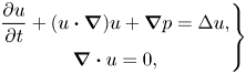 \begin{equation} \left.\begin{gathered} \frac{\partial u}{\partial t} + (u\boldsymbol{\cdot}\boldsymbol{\nabla})u + \boldsymbol{\nabla} p = \Delta u, \\ \boldsymbol{\nabla}\boldsymbol{\cdot} u = 0, \end{gathered}\right\} \end{equation}
where  $u(x,t):\mathbb {R}^3\times [0,T]\rightarrow \mathbb {R}^3$ and $p(x,t):\mathbb {R}^3\times [0,T]\rightarrow \mathbb {R}$ are, respectively, the velocity and pressure fields. The viscosity is set to one for convenience and the initial velocity $u(x,0):=\boldsymbol{u}_0(x)$ satisfies $\boldsymbol {\nabla }\boldsymbol {\cdot } \boldsymbol{u}_0=0$ and $\boldsymbol{u}_0\in L^2(\mathbb {R}^3)$, i.e.
 \begin{equation} \left|\mkern-2mu\left|\boldsymbol{u}_0\right|\mkern-2mu\right|_{L^2(\mathbb{R}^3)}^2:=\int_{\mathbb{R}^3}|\boldsymbol{u}_0|^2\,{\textrm{d} x} < \infty. \end{equation}
 The Cauchy problem of (1.1) is an outstanding issue in classical mechanics and applied mathematics. The pioneering studies by Leray (Reference Leray1934) and Hopf (Reference Hopf1951) have established the existence of a weak (Leray–Hopf) solution(s) that attains the initial velocity  $\boldsymbol{u}_0(x)$ in the $L^2$ sense and satisfies the energy inequality
 \begin{equation} \left|\mkern-2mu\left|u\right|\mkern-2mu\right|_{L^2(\mathbb{R}^3)}^2 + 2\int_0^T\left|\mkern-2mu\left|\boldsymbol{\nabla} u\right|\mkern-2mu\right|_{L^2(\mathbb{R}^3)}^2\, \mathrm{d}t \le \left|\mkern-2mu\left|\boldsymbol{u}_0\right|\mkern-2mu\right|_{L^2(\mathbb{R}^3)}^2, \end{equation}
for all  $T>0$. However, smoothness and uniqueness (regularity) of such solutions are not known. What has been known since Leray's work is that if a Leray–Hopf solution becomes singular at $t=T_*$, then
 \begin{equation} \left|\mkern-2mu\left|u\right|\mkern-2mu\right|_{L^s(\mathbb{R}^3)} \ge \frac{c}{(T_*-t)^{(s-3)/2s}}, \quad \mbox{for}\ s>3,\ \mbox{as}\ t\to T_*, \end{equation}
where  $c>0$ is an absolute constant. Apparently, the borderline case $s=3$ is not included in (1.4). This case turns out to be critical, due to the criticality of the $L^3(\mathbb {R}^3)$ norm, and has recently been addressed by Tao (Reference Tao2019) in the following singularity criterion (see also the regularity criterion of Escauriaza, Seregin & Šverák (Reference Escauriaza, Seregin and Šverák2003) below):
 \begin{equation} \limsup_{t\to T_*}\frac{\left|\mkern-2mu\left|u\right|\mkern-2mu\right|_{L^3(\mathbb{R}^3)}}{\left(\log\log\log1/(T_*-t)\right)^c} = \infty, \end{equation}
for an absolute constant  $c>0$.
To date, regularity has only been established under certain preconditions, known as regularity criteria. The most well-known results are the classical criteria
 \begin{equation} \int_0^T\left|\mkern-2mu\left|u\right|\mkern-2mu\right|_{L^s(\mathbb{R}^3)}^{2s/(s-3)}\,\mathrm{d}t < \infty, \quad \mbox{for}\ s>3, \end{equation}
of Ladyzhenskaya (Reference Ladyzhenskaya1967), Prodi (Reference Prodi1959) and Serrin (Reference Serrin1962), and
 \begin{equation} \mathop{\mathrm{esssup}}\limits_{(0,T)}\left|\mkern-2mu\left|u\right|\mkern-2mu\right|_{L^3(\mathbb{R}^3)} < \infty \end{equation}
of Escauriaza et al. (Reference Escauriaza, Seregin and Šverák2003), for regularity up to  $t=T$. Note that Tao's singularity criterion (1.5) represents a quantitative improvement to (1.7), albeit by an exceedingly weak triple logarithmic factor. This is a convincing confirmation of the critical and optimal status of (1.7). Criterion (1.6) remains valid when the norm $\left |\mkern -2mu\left |u\right |\mkern -2mu\right |_{L^s(\mathbb {R}^3)}$ is replaced by its scale-equivalent but marginally weaker counterpart $\left |\mkern -2mu\left |p\right |\mkern -2mu\right |_{L^{s/2}(\mathbb {R}^3)}^{1/2}$. Indeed the criterion
 \begin{equation} \int_0^T\left|\mkern-2mu\left|p\right|\mkern-2mu\right|_{L^s(\mathbb{R}^3)}^{2s/(2s-3)}\mathrm{d}t < \infty, \quad \mbox{for}\ s>3/2, \end{equation}
was derived by Chae & Lee (Reference Chae and Lee2001) and Berselli & Galdi (Reference Berselli and Galdi2002).
Evidently, the above criteria imply that singularity would require both  $|u|$ and $|p|$ to become infinite. We could furthermore expect all three quantities $|u|$, $|p|$ and $|\boldsymbol {\nabla } p|$ to diverge concurrently at points where the flow becomes singular. The reason is that fluid particles are locally accelerated by $-\boldsymbol {\nabla } p$, which, because of criterion (1.8), may become infinite only if $p$ does. More precisely, let $T_\ast >0$ be the first singularity time, then it is necessary that $\|u\|_{L^r}\to \infty$ for some $r\geqslant 3$. Setting
 \begin{equation} \varOmega(t):=\{x:|u(x,t)|>c_1 \|u\|_{L^r}\} \end{equation}
as in Tran & Yu (Reference Tran and Yu2017a), it has been shown in Lemma 3 there that as long as  $\|p\|_{L^{3/2}(\varOmega (t))} < c_0$ for some constant $c_0$, the solution remains regular. As the volume $|\varOmega (t)|$ necessarily vanishes in the limit $t\to T_\ast$, it must be the case that $\sup _{\varOmega (t)}|p(\cdot ,t)|\to \infty$ as $t\to T_\ast$. A similar blow-up criterion can be derived for $\boldsymbol {\nabla } p$, leading to the conclusion that $\sup _{\varOmega (t)}|\nabla p(\cdot ,t)|\to \infty$ as well.
There is no guarantee that in the singularity limit  $t\to T_\ast$, $\varOmega (t)$ would reduce to a set with some simple geometric structures. Nonetheless, Choe, Wolf & Yang (Reference Choe, Wolf and Yang2020) have shown that under favourable conditions (considered in the present study and further elaborated in § 4.2), a finite collection of isolated points would be the only outcome for the limiting singularity set. Hence, it is reasonable to focus on a single ‘singular point’. Let $x=x_0$ be such a point where the flow becomes singular at a finite time $T_\ast$. We would have both $|u(x_0)|=\infty$ and $|\boldsymbol {\nabla } p(x_0)|=\infty$, and furthermore $p(x_0)=-\infty$. Here $p(x_0)=-\infty$ and not $p(x_0)=+\infty$, because fluid particles are accelerated as they are heading towards lower and not higher pressure. For a rigorous and detailed account of how the pressure would blow up ( $p\to -\infty$) in Navier–Stokes singularity, see Seregin & Šverák (Reference Seregin and Šverák2002).
The requirement of simultaneous blow-up of  $|u|$ and $|p|$ at a singular point gives a relatively clear picture of Navier–Stokes singularity: high-velocity fluid particles crashing upon a global pressure minimum (or multiple minima) that decreases to negative infinity in a finite time. Hence, the spatial correlation between $|u|$ and $|p|$ is a matter of utmost importance, which nonetheless has never been addressed in the literature. This appears to be an oversight with possible groundbreaking implications.
This study examines the growth rate of  $\left |\mkern -2mu\left |u\right |\mkern -2mu\right |_{L^q(\mathbb {R}^3)}$, for $q\ge 3$, which controls the flow regularity. With the stringent constraint on singularity development described above in mind, we present and discuss regularity criteria that encapsulate the velocity–pressure correlation as an essential feature. The results confirm that exceedingly high velocity–pressure correlation is required for strong local momentum growth. Furthermore, it is shown that as long as local velocity maxima and pressure minima are mutually exclusive then singularity is unrealisable. We examine the plausibility of the derived criteria for flow scenarios satisfying the critical scaling of the Navier–Stokes equations and find that singularity may not develop while respecting such scaling.
2. Motivation
The evolution of the local energy  $|u|^2/2$ is governed by
 \begin{equation} \frac{\partial}{\partial t}\frac{|u|^2}{2} + u\boldsymbol{\cdot}\boldsymbol{\nabla}\frac{|u|^2}{2} + u\boldsymbol{\cdot}\boldsymbol{\nabla} p = \varDelta\frac{|u|^2}{2}-|\boldsymbol{\nabla} u|^2. \end{equation}
Multiplying (2.1) by  $|u|^{q-2}$ and integrating the resulting equation over $\mathbb {R}^3$ we obtain the evolution equation for $\left |\mkern -2mu\left |u\right |\mkern -2mu\right |_{L^q(\mathbb {R}^3)}:=\left |\mkern -2mu\left |u\right |\mkern -2mu\right |_{L^q}$:
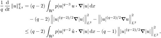 \begin{align} \frac{1}{q}\,\frac{\mathrm{d}}{\mathrm{d}t}\left|\mkern-2mu\left|u\right|\mkern-2mu\right|_{L^q}^q &= (q-2)\int_{\mathbb{R}^3} p|u|^{q-3}\,u\boldsymbol{\cdot}\boldsymbol{\nabla}|u|\,{\textrm{d} x} \nonumber\\ &\quad - (q-2)\left|\mkern-2mu\left||u|^{(q-2)/2}\boldsymbol{\nabla}|u|\right|\mkern-2mu\right|_{L^2}^2 - \left|\mkern-2mu\left||u|^{(q-2)/2}\boldsymbol{\nabla} u\right|\mkern-2mu\right|_{L^2}^2 \nonumber\\ &\le (q-2)\int_{\mathbb{R}^3} p|u|^{q-2}\,\hat{u}\boldsymbol{\cdot}\boldsymbol{\nabla}|u|\,{\textrm{d} x} - (q-1)\left|\mkern-2mu\left||u|^{(q-2)/2}\boldsymbol{\nabla}|u|\right|\mkern-2mu\right|_{L^2}^2, \end{align}
where  $\hat {u}:=u/|u|$ is the unit vector along streamlines.
The integral in the driving term in (2.2) may be estimated in a variety of ways. To facilitate a comparison with its dissipation counterpart, a commonly used estimate via the Cauchy–Schwarz inequality is
 \begin{equation} \int_{\mathbb{R}^3} p|u|^{q-2}\,\hat{u}\boldsymbol{\cdot}\boldsymbol{\nabla}|u|\, {\textrm{d} x} \le \left(\int_{\mathbb{R}^3} p^2|u|^{q-2}\, {\textrm{d} x}\right)^{1/2} \left|\mkern-2mu\left||u|^{(q-2)/2}\boldsymbol{\nabla}|u|\right|\mkern-2mu\right|_{L^2}. \end{equation}
When dealing with estimates involving  $p$, such as the integral on the right-hand side of the above equation, it is customary to rely on the Calderón–Zygmund inequality $\left |\mkern -2mu\left |p\right |\mkern -2mu\right |_{L^s}\le c_s\left |\mkern -2mu\left |u\right |\mkern -2mu\right |_{L^{2s}}^2$, for $s\in (1,\infty )$, as virtually no other quantitative knowledge of $p$ is available (for a mathematical exposition centred around the Poisson equation for the pressure, see Li & Zhang (Reference Li and Zhang2019)). Upon application of this inequality, together with the Hölder inequality, one obtains
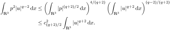 \begin{align} \int_{\mathbb{R}^3} p^2|u|^{q-2}\,{\textrm{d} x} &\le \left(\int_{\mathbb{R}^3} |p|^{(q+2)/2}\,{\textrm{d} x}\right)^{4/(q+2)} \left(\int_{\mathbb{R}^3} |u|^{q+2}\, {\textrm{d} x}\right)^{(q-2)/(q+2)} \nonumber\\ &\le c^2_{{(q+2)/2}}\int_{\mathbb{R}^3} |u|^{q+2}\,{\textrm{d} x}. \end{align}
In effect, one replaces  $|p|$ by $|u|^2$ under the integral sign. But doing so results in an unrecoverable loss of velocity–pressure correlation, which is a favourable feature for regularity. In order to appreciate the extent of this loss, consider the following illustration which motivates the present study.
Let  $B(x_0,\delta )$ be a ball centred at $x_0$ with radius $\delta$ and $x'_0\in B(x_0,\delta )$. Let $\psi (x)$ and $\phi (x)$ be two singular distributions in $B(x_0,\delta )$ given by
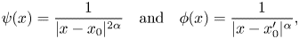 \begin{equation} \psi(x) = \frac{1}{|x-x_0|^{2\alpha}}\quad \mbox{and}\quad \phi(x) = \frac{1}{|x-x'_0|^\alpha}, \end{equation}
for some  $\alpha \ge 1$. Figure 1 illustrates in the spherical coordinate setting the locations of the (singular) peaks of $\psi$ and $\phi$ at $x=x_0$ and $x=x'_0$, respectively. The origin of the system is conveniently set at $x_0$. The separation of the singular peaks of $\psi (x)$ and $\phi (x)$ is denoted by $\epsilon :=|x_0-x'_0|$. The parameter $\epsilon$ may be used as a simple measure of the correlation between $\psi (x)$ and $\phi (x)$ in $B$. When $\epsilon =0$, the correlation is said to be perfect. High but imperfect correlation corresponds to small but non-zero $\epsilon$. For most of this study, we consider $\alpha =1$, so that $\psi$ and $\phi$, when likened respectively to $|p|$ and $|u|$, correspond to the critical scaling of the Navier–Stokes equations. Now let $\chi (x):=\psi ^{1/4}(x)\phi ^{1/2}(x)$. As can be seen from figure 1, $\chi$ is given in terms of $r$,
$r$,  $\epsilon$ and $\theta$ by $\chi =r^{-1/2}(r^2+\epsilon ^2-2r\epsilon \cos \theta )^{-1/4}$. For $\epsilon >0$, $\left |\mkern -2mu\left |\chi \right |\mkern -2mu\right |_{L^3(B)}^3$ may be estimated as follows:
 \begin{align} \left|\mkern-2mu\left|\chi\right|\mkern-2mu\right|_{L^3(B)}^3 &= 2{\rm \pi}\int_0^\delta\int_0^{\rm \pi}\frac{r^2\sin\theta\,\mathrm{d}\theta\,\mathrm{d} r} {r^{3/2}(r^2+\epsilon^2-2r\epsilon\cos\theta)^{3/4}} \nonumber\\ &=\frac{4{\rm \pi}}{\xi}\int_0^1\frac{|\rho+\xi|^{1/2}-|\rho-\xi|^{1/2}} {\rho^{1/2}}\,\mathrm{d}\rho \nonumber\\ &=\frac{4{\rm \pi}}{\xi}\int_0^1\frac{|\rho+\xi|-|\rho-\xi|} {\rho^{1/2}\left(|\rho+\xi|^{1/2}+|\rho-\xi|^{1/2}\right)} \,\mathrm{d}\rho \nonumber\\ &\le\frac{8{\rm \pi}}{\xi}\int_0^\xi{\mathrm{d}}\rho + 8{\rm \pi}\int_\xi^1\frac{\mathrm{d}\rho}{\rho} = 8{\rm \pi}(1 + \log(1/\xi)), \end{align}
where  $\xi :=\epsilon /\delta$. It is clear that $\left |\mkern -2mu\left |\chi \right |\mkern -2mu\right |_{L^3(B)}<\infty$ for $\xi >0$. Furthermore, in the limit of small $\xi$, $\left |\mkern -2mu\left |\chi \right |\mkern -2mu\right |_{L^3(B)}^3$ diverges logarithmically as expected. Obviously, higher correlation gives rise to stronger mixed norm $\left |\mkern -2mu\left |\chi \right |\mkern -2mu\right |_{L^3(B)}$. Here neither $\psi ^{1/2}\in L^3(B)$ nor $\phi \in L^3(B)$, yet $\chi$, which has the same scaling as $\phi$ and $\psi ^{1/2}$, can be in $L^3(B)$ for imperfect correlation. In fact, we have $\chi \in L^{6^-}(B)$ when $\xi >0$, and the loss of optimality is enormous if $\psi$ and $\phi$ are decoupled in estimation. For example, in the usual Cauchy–Schwarz estimate $\left |\mkern -2mu\left |\chi \right |\mkern -2mu\right |_{L^4(B)}\le \left |\mkern -2mu\left |\psi \right |\mkern -2mu\right |_{L^2(B)}^{1/4}\left |\mkern -2mu\left |\phi \right |\mkern -2mu\right |_{L^4(B)}^{1/2}$, the left-hand side is finite while the right-hand side strongly diverges as $\left |\mkern -2mu\left |\psi \right |\mkern -2mu\right |_{L^2(B)}$ and $\left |\mkern -2mu\left |\phi \right |\mkern -2mu\right |_{L^4(B)}$ each diverges. This illustrates the significance of the correlation between $\psi$ and $\phi$ in determining the magnitude of their mixed norms.

Figure 1. An illustration of the respective locations of (singular) peaks of  $\psi$ and $\phi$ at $x_0$ and $x'_0$ in $B(x_0,\delta )$. Here, $\epsilon := |x_0-x'_0|$ is the separation of the peaks. For a given point $x\in B(x_0,\delta )$, let $r := |x-x_0|$ and $r' := |x-x'_0|$. The latter is given in terms of $\epsilon$, $r$ and the polar angle $\theta$ by $r'=(\epsilon ^2+r^2-2\epsilon r\cos \theta )^{1/2}$.
3. Results
3.1. Velocity–pressure correlation
Let  $U(t,q)>0$ be a reference velocity that can depend on time (and $q$). Following Tran & Yu (Reference Tran and Yu2016, Reference Tran and Yu2018, Reference Tran and Yu2019), we partition $\mathbb {R}^3$ into high- and low-velocity regions $\varOmega (t,q)$ and $\varOmega ^c(t,q)$ by $\varOmega := \{x\mid |u(x,t)| > U\}$ and $\varOmega ^c:=\mathbb {R}^3\setminus \varOmega$. This partition allows us to write (2.2) in the form
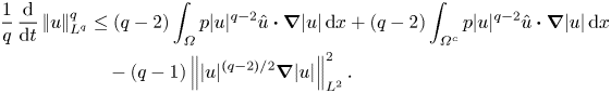 \begin{align} \frac{1}{q}\,\frac{\mathrm{d}}{\mathrm{d}t}\left|\mkern-2mu\left|u\right|\mkern-2mu\right|_{L^q}^q&\le (q-2)\int_\varOmega p|u|^{q-2}\hat{u}\boldsymbol{\cdot}\boldsymbol{\nabla}|u|\, {\textrm{d} x} + (q-2)\int_{\varOmega^c}p|u|^{q-2}\hat{u}\boldsymbol{\cdot}\boldsymbol{\nabla}|u|\,{\textrm{d} x} \nonumber\\ &\quad - (q-1)\left|\mkern-2mu\left||u|^{(q-2)/2}\boldsymbol{\nabla}|u|\right|\mkern-2mu\right|_{L^2}^2. \end{align}
The integral over  $\varOmega ^c$ in (3.1), which represents the contribution to the driving term from the low-velocity region $\varOmega ^c$, can be bounded above by
 \begin{align} \int_{\varOmega^c} p|u|^{q-2}\hat{u}\boldsymbol{\cdot}\boldsymbol{\nabla}|u|\, {\textrm{d} x} &\le U^{(q-2)/2}\left|\mkern-2mu\left|p\right|\mkern-2mu\right|_{L^2(\varOmega^c)}\left|\mkern-2mu\left||u|^{(q-2)/2}\boldsymbol{\nabla}|u|\right|\mkern-2mu\right|_{L^2(\varOmega^c)}\nonumber\\ &\le \frac{1}{2}\left|\mkern-2mu\left||u|^{(q-2)/2}\boldsymbol{\nabla}|u|\right|\mkern-2mu\right|_{L^2}^2, \end{align}
where we have used the Cauchy–Schwarz inequality and set
 \begin{equation} U := \left(\frac{R}{2}\frac{\left|\mkern-2mu\left||u|^{(q-2)/2}\boldsymbol{\nabla}|u|\right|\mkern-2mu\right|_{L^2}}{\left|\mkern-2mu\left|p\right|\mkern-2mu\right|_{L^2}}\right)^{2/(q-2)} \quad \mbox{and}\quad R:= \frac{\left|\mkern-2mu\left||u|^{(q-2)/2}\boldsymbol{\nabla}|u|\right|\mkern-2mu\right|_{L^2}}{ \left|\mkern-2mu\left||u|^{(q-2)/2}\boldsymbol{\nabla}|u|\right|\mkern-2mu\right|_{L^2(\varOmega^c)}}. \end{equation}
Substituting the above estimate into (3.1) yields
 \begin{equation} \frac{1}{q}\,\frac{\mathrm{d}}{\mathrm{d}t}\left|\mkern-2mu\left|u\right|\mkern-2mu\right|_{L^q}^q \le(q-2)\int_{\varOmega} p|u|^{q-2}\,\hat{u}\boldsymbol{\cdot}\boldsymbol{\nabla}|u|\,{\textrm{d} x} - \frac{q}{2}\left|\mkern-2mu\left||u|^{(q-2)/2}\boldsymbol{\nabla}|u|\right|\mkern-2mu\right|_{L^2}^2. \end{equation}
Remark We note that the definition of  $\varOmega$ (and $\varOmega ^c$) is implicit through
 \begin{equation} \varOmega := \left\{x\mid |u(x,t)| >\left(\frac{\left|\mkern-2mu\left||u|^{(q-2)/2}\boldsymbol{\nabla}|u|\right|\mkern-2mu\right|_{L^2}^2}{2\left|\mkern-2mu\left||u|^{(q-2)/2} \boldsymbol{\nabla}|u|\right|\mkern-2mu\right|_{L^2(\varOmega^c)}\left|\mkern-2mu\left|p\right|\mkern-2mu\right|_{L^2}}\right)^{2/(q-2)} \right\}. \end{equation}
Nonetheless,  $\varOmega$ is well defined by an argument similar to that in § 3 of Tran & Yu (Reference Tran and Yu2018). A sketch of proof of this fact is presented in appendix A for completeness.
Remark The number  $R^2\ge 1$ is the ratio of the total dissipation to that in the low-velocity region $\varOmega ^c$.
Applying the Sobolev inequality  $\left |\mkern -2mu\left |h\right |\mkern -2mu\right |_{L^6}\le c_0\left |\mkern -2mu\left |\boldsymbol {\nabla } h\right |\mkern -2mu\right |_{L^2}$, where $c_0=(2/{\rm \pi} )^{2/3}/\sqrt 3$ (cf. Talenti Reference Talenti1976), to $h=|u|^{q/2}$ yields
 \begin{equation} \frac{2}{c_0q}\left|\mkern-2mu\left|u\right|\mkern-2mu\right|_{L^{3q}}^{q/2}\le\left|\mkern-2mu\left||u|^{(q-2)/2}\boldsymbol{\nabla}|u|\right|\mkern-2mu\right|_{L^2}. \end{equation}
This means that
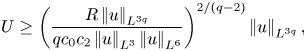
 \begin{equation} U \ge \left(\frac{R\left|\mkern-2mu\left|u\right|\mkern-2mu\right|_{L^{3q}}}{c_0q\left|\mkern-2mu\left|p\right|\mkern-2mu\right|_{L^2}}\right)^{2/(q-2)}\left|\mkern-2mu\left|u\right|\mkern-2mu\right|_{L^{3q}}, \end{equation}
which is comparable to  $\left |\mkern -2mu\left |u\right |\mkern -2mu\right |_{L^{3q}}$ in the limit of large $q$. For moderate $q$, the Calderón–Zygmund inequality $\left |\mkern -2mu\left |p\right |\mkern -2mu\right |_{L^2}\le c_2\left |\mkern -2mu\left |u\right |\mkern -2mu\right |_{L^4}^2$ and the interpolation inequality $\left |\mkern -2mu\left |u\right |\mkern -2mu\right |_{L^4}^2\le \left |\mkern -2mu\left |u\right |\mkern -2mu\right |_{L^3}\left |\mkern -2mu\left |u\right |\mkern -2mu\right |_{L^6}$ allow us to write
 \begin{equation} U \ge \left(\frac{R\left|\mkern-2mu\left|u\right|\mkern-2mu\right|_{L^{3q}}}{qc_0c_2\left|\mkern-2mu\left|u\right|\mkern-2mu\right|_{L^3}\left|\mkern-2mu\left|u\right|\mkern-2mu\right|_{L^6}}\right)^{2/(q-2)} \left|\mkern-2mu\left|u\right|\mkern-2mu\right|_{L^{3q}}, \end{equation}
which can be far greater than  $\left |\mkern -2mu\left |u\right |\mkern -2mu\right |_{L^{3q}}$, provided that $R\left |\mkern -2mu\left |u\right |\mkern -2mu\right |_{L^{3q}}/\left |\mkern -2mu\left |u\right |\mkern -2mu\right |_{L^3}\left |\mkern -2mu\left |u\right |\mkern -2mu\right |_{L^6}\gg 1$. This condition holds in the limit of large $\left |\mkern -2mu\left |u\right |\mkern -2mu\right |_{L^{3q}}$ if $\left |\mkern -2mu\left |u\right |\mkern -2mu\right |_{L^3}$ grows relatively weakly in that limit. In any case, the present reference velocity $U$ is significantly more optimal than its previous counterpart, which is only comparable to $\left |\mkern -2mu\left |u\right |\mkern -2mu\right |_{L^{3q-6}}$.
The driving set  $\varOmega$ may be further localised by a condition on $p$ in $\varOmega$ similar to $|u|>U$. Indeed, defining $\varOmega ' := \varOmega \cap \{x\mid |p(x,t)| \le P(t)\}$, where $P(t)$ is some reference pressure, then we can apply the Cauchy–Schwarz inequality to obtain
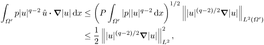 \begin{align} \int_{\varOmega'}p|u|^{q-2}\,\hat{u}\boldsymbol{\cdot}\boldsymbol{\nabla}|u|\,{\textrm{d} x} &\le \left(P\int_{\varOmega'}|p||u|^{q-2}\,{\textrm{d} x}\right)^{1/2} \left|\mkern-2mu\left||u|^{(q-2)/2}\boldsymbol{\nabla}|u|\right|\mkern-2mu\right|_{L^2(\varOmega')}\nonumber\\ &\le \frac{1}{2}\left|\mkern-2mu\left||u|^{(q-2)/2}\boldsymbol{\nabla}|u|\right|\mkern-2mu\right|_{L^2}^2, \end{align}
as long as
 \begin{equation} P\leqslant \frac{R'^2\left|\mkern-2mu\left||u|^{(q-2)/2}\boldsymbol{\nabla}|u|\right|\mkern-2mu\right|_{L^2}^2}{4 \int_{\varOmega'}|p||u|^{q-2}\, {\textrm{d} x}} \quad \mbox{with}\ R':=\frac{\left|\mkern-2mu\left||u|^{(q-2)/2}\boldsymbol{\nabla}|u|\right|\mkern-2mu\right|_{L^2}} {\left|\mkern-2mu\left||u|^{(q-2)/2}\boldsymbol{\nabla}|u|\right|\mkern-2mu\right|_{L^2(\varOmega')}}\ge 1. \end{equation}
The existence of such  $\varOmega '$ can be established in a similar manner to that of $\varOmega$ above.
Substituting the above estimate into (3.4) yields
 \begin{equation} \frac{1}{q}\,\frac{\mathrm{d}}{\mathrm{d}t}\left|\mkern-2mu\left|u\right|\mkern-2mu\right|_{L^q}^q \le (q-2)\int_{\varOmega_0} p|u|^{q-2}\,\hat{u}\boldsymbol{\cdot}\boldsymbol{\nabla}|u|\, {\textrm{d} x} - \frac{q}{4}\left|\mkern-2mu\left||u|^{(q-2)/2}\boldsymbol{\nabla}|u|\right|\mkern-2mu\right|_{L^2}^2, \end{equation}
where  $\varOmega _0:=\varOmega \setminus \varOmega '$.
Remark By the Sobolev and Calderón–Zygmund inequalities, together with the interpolation inequality  $\left |\mkern -2mu\left |u\right |\mkern -2mu\right |_{L^q}\le \left |\mkern -2mu\left |u\right |\mkern -2mu\right |_{L^3}^{2/(q-1)}\left |\mkern -2mu\left |u\right |\mkern -2mu\right |_{L^{3q}}^{(q-3)/(q-1)}$, we have
 \begin{equation} P \ge \frac{R'^2\left|\mkern-2mu\left|u\right|\mkern-2mu\right|_{L^{3q}}^q}{c_0^2q^2c_{q/2}^2\left|\mkern-2mu\left|u\right|\mkern-2mu\right|_{L^q}^q} \ge \frac{R'^2\left|\mkern-2mu\left|u\right|\mkern-2mu\right|_{L^{3q}}^q}{c_0^2q^2c_{q/2}^2\left|\mkern-2mu\left|u\right|\mkern-2mu\right|_{L^3}^{2q/(q-1)}\left|\mkern-2mu\left|u\right|\mkern-2mu\right|_{L^{3q}}^{q(q-3)/(q-1)}} = \frac{R'^2\left|\mkern-2mu\left|u\right|\mkern-2mu\right|_{L^{3q}}^{2q/(q-1)}}{c_0^2q^2c_{q/2}^2\left|\mkern-2mu\left|u\right|\mkern-2mu\right|_{L^3}^{2q/(q-1)}}. \end{equation}
In the limit of large  $\left |\mkern -2mu\left |u\right |\mkern -2mu\right |_{L^{3q}}$, $P$ is comparable to $\left |\mkern -2mu\left |u\right |\mkern -2mu\right |_{L^{3q}}^2$ if $\left |\mkern -2mu\left |u\right |\mkern -2mu\right |_{L^3}$ grows relatively weakly. This remains true for moderate $q$.
$q$.
Remark It is apparent that  $|u|$ and $|p|$ are required to be highly correlated in the reduced driving set $\varOmega _0$: both $|u|^2$ and $|p|$ are of the order of $\left |\mkern -2mu\left |u\right |\mkern -2mu\right |_{L^{3q}}^2$ or greater.
Let  $|\varOmega |$ and $|\varOmega _0|$ denote the measures of $\varOmega$ and $\varOmega _0$, respectively. By the very definitions of $\varOmega$ and $\varOmega _0$ we have
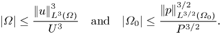 \begin{equation} |\varOmega| \le \frac{\left|\mkern-2mu\left|u\right|\mkern-2mu\right|_{L^3(\varOmega)}^3}{U^3}\quad\mbox{and}\quad |\varOmega_0| \le \frac{\left|\mkern-2mu\left|p\right|\mkern-2mu\right|_{L^{3/2}(\varOmega_0)}^{3/2}}{P^{3/2}}. \end{equation}
These measures diminish rapidly as  $\left |\mkern -2mu\left |u\right |\mkern -2mu\right |_{L^{3q}}$ increases. If $|\varOmega _0(T,q)|=0$, then the reduced driving term in (3.11) vanishes, $\left |\mkern -2mu\left |u\right |\mkern -2mu\right |_{L^q}$ decays and regularity persists beyond $t=T$. This possibility seems unlikely but nonetheless may not be ruled out.
In passing, it is worth emphasising that the dependence on  $t$ of dynamical entities, including the sets $\varOmega$, $\varOmega '$ and $\varOmega _0$, has been suppressed for clarity. This practice will be continued for the remainder of this study.
3.2. Regularity criteria
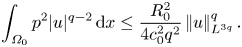
In this section we derive and discuss several regularity criteria. Returning to (3.11) we have
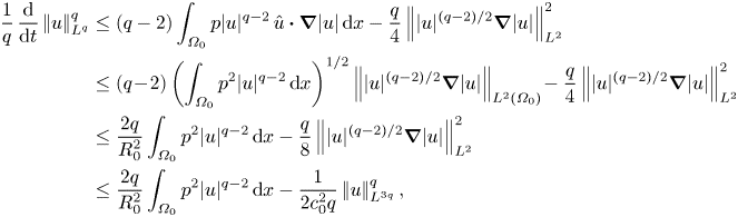 \begin{align} \frac{1}{q}\,\frac{\mathrm{d}}{\mathrm{d}t}\left|\mkern-2mu\left|u\right|\mkern-2mu\right|_{L^q}^q &\le(q-2)\int_{\varOmega_0} p|u|^{q-2}\,\hat{u}\boldsymbol{\cdot}\boldsymbol{\nabla}|u|\, {\textrm{d} x} - \frac{q}{4}\left|\mkern-2mu\left||u|^{(q-2)/2}\boldsymbol{\nabla}|u|\right|\mkern-2mu\right|_{L^2}^2 \nonumber\\ &\le (q\!-\!2)\left(\int_{\varOmega_0}p^2|u|^{q-2}\,{\textrm{d} x}\right)^{1/2} \left|\mkern-2mu\left||u|^{(q-2)/2}\boldsymbol{\nabla}|u|\right|\mkern-2mu\right|_{L^2(\varOmega_0)} \!- \frac{q}{4}\left|\mkern-2mu\left||u|^{(q-2)/2}\boldsymbol{\nabla}|u|\right|\mkern-2mu\right|_{L^2}^2 \nonumber\\ &\le \frac{2q}{R_0^2}\int_{\varOmega_0}p^2|u|^{q-2}\, {\textrm{d} x} - \frac{q}{8}\left|\mkern-2mu\left||u|^{(q-2)/2}\boldsymbol{\nabla}|u|\right|\mkern-2mu\right|_{L^2}^2 \nonumber\\ &\le \frac{2q}{R_0^2}\int_{\varOmega_0}p^2|u|^{q-2}\,{\textrm{d} x} - \frac{1}{2c_0^2q}\left|\mkern-2mu\left|u\right|\mkern-2mu\right|_{L^{3q}}^q, \end{align}
where  $R_0:=\left |\mkern -2mu\left ||u|^{(q-2)/2}\boldsymbol {\nabla }|u|\right |\mkern -2mu\right |_{L^2}/\left |\mkern -2mu\left ||u|^{(q-2)/2}\boldsymbol {\nabla }|u|\right |\mkern -2mu\right |_{L^2(\varOmega _0)}\ge 1$ and the Sobolev inequality has been used. For a quantitative description of the velocity–pressure correlation in further analysis, we define the correlation coefficient $\varGamma _q$ by
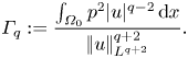 \begin{equation} \varGamma_q := \frac{\int_{\varOmega_0}p^2|u|^{q-2}\,{\textrm{d} x}}{\left|\mkern-2mu\left|u\right|\mkern-2mu\right|_{L^{q+2}}^{q+2}}. \end{equation}
This enables us to present modified versions of the classical result (1.6) and its recent improvements by Tran & Yu (Reference Tran and Yu2017b) in the following theorem.
Theorem 3.1 Let  $\{u,p\}$ be a Leray–Hopf solution to the initial-value problem of the three-dimensional Navier–Stokes equations. Assume that $\{u,p\}$ is smooth on the time interval $(0,T)$. Then the solution remains smooth up to and beyond $t=T$, if one of the following holds.
(a) For some $s\in (3,\infty )$,
(3.16)\begin{equation} \int_0^T\left(\frac{\varGamma_s}{R_0^2}\right)^{s/(s-3)} \left|\mkern-2mu\left|u\right|\mkern-2mu\right|_{L^s}^{2s/(s-3)}\,\mathrm{d} t < \infty. \end{equation}
$s\in (3,\infty )$,
(3.16)\begin{equation} \int_0^T\left(\frac{\varGamma_s}{R_0^2}\right)^{s/(s-3)} \left|\mkern-2mu\left|u\right|\mkern-2mu\right|_{L^s}^{2s/(s-3)}\,\mathrm{d} t < \infty. \end{equation}(b) For some
$s\in (3,5]$,
(3.17)\begin{equation} \int_0^T\left(\frac{\varGamma_3}{R_0^2}\right)^{(9-s)/(2s-6)} \frac{\left|\mkern-2mu\left|u\right|\mkern-2mu\right|_{L^s}^{2s/(s-3)}}{\left|\mkern-2mu\left|u\right|\mkern-2mu\right|_{L^3}^3}\,\mathrm{d} t < \infty. \end{equation}(c) For some
$s>5$,
(3.18)\begin{equation} \int_0^T\frac{\varGamma_3}{R_0^2}\, \frac{\left|\mkern-2mu\left|u\right|\mkern-2mu\right|_{L^s}^{2s/(s-3)}}{\left|\mkern-2mu\left|u\right|\mkern-2mu\right|_{L^3}^{6/(s-3)}}\,\mathrm{d} t < \infty. \end{equation}


A proof of this theorem is given in appendix B.
Remark Criterion (3.16) features a refinement over the classical result (1.6). On the one hand, application of the Hölder inequality and the Calderón–Zygmund inequality leads to  $\varGamma _s\leqslant C$ for some absolute constant $C$. Together with $R_0\geqslant 1$, this implies that the factor $(\varGamma _s/R_0^2)^{s/(s-3)}$ is bounded by an absolute constant, and (1.6) implies (3.16). On the other hand, as we can see from its very definition (3.14), $\varGamma _s$ is small when the correlation between $|u|$ and $|p|$ is low. Further discussion of this favourable feature is delayed to § 4.2.
Criteria (3.17) and (3.18) further refine (3.16), as each has two improvements over their classical counterpart (1.6). One is the factor concerning  $\varGamma _3$ and the other is the factor concerning $\left |\mkern -2mu\left |u\right |\mkern -2mu\right |_{L^3}$.
In comparison with (3.16), (3.17) and (3.18) have the favourable factors  $1/\left |\mkern -2mu\left |u\right |\mkern -2mu\right |_{L^3}^3$ and $1/\left |\mkern -2mu\left |u\right |\mkern -2mu\right |_{L^3}^{6/(s-3)}$, respectively. However, it is not known with certainty whether their optimality compares favourably to that of (3.16) since we lack a quantitative knowledge of the coefficients $\varGamma _3$ and $\varGamma _q$. The answer to this question undoubtedly requires a mathematical theory of the velocity–pressure correlation beyond the present work, which provides rather qualitative treatment of this correlation (see further examination in § 4).
Criteria similar to (3.16), (3.17) and (3.18), albeit expressible in terms of  $\left |\mkern -2mu\left |p\right |\mkern -2mu\right |_{L^s(\varOmega _0)}$, for $s>3/2$, can be derived by the same method. Here we present the result for $s\in (3/2,9/4]$ only. By Hölder's inequality we have
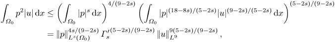 \begin{align} \int_{\varOmega_0}p^2|u|\,{\textrm{d} x} &\le \left(\int_{\varOmega_0}|p|^s\,{\textrm{d} x}\right)^{4/(9-2s)} \left(\int_{\varOmega_0}|p|^{(18-8s)/(5-2s)}|u|^{(9-2s)/(5-2s)}\,{\textrm{d} x}\right)^{(5-2s)/(9-2s)}\nonumber\\ &= \left|\mkern-2mu\left|p\right|\mkern-2mu\right|_{L^s(\varOmega_0)}^{4s/(9-2s)}{\varGamma_s'}^{(5-2s)/(9-2s)}\left|\mkern-2mu\left|u\right|\mkern-2mu\right|_{L^9}^{9(5-2s)/(9-2s)}, \end{align}
which is valid for  $s\le 9/4$. Here
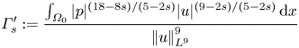 \begin{equation} \varGamma_s' := \frac{\int_{\varOmega_0}|p|^{(18-8s)/(5-2s)}|u|^{(9-2s)/(5-2s)}\, {\textrm{d} x}}{\left|\mkern-2mu\left|u\right|\mkern-2mu\right|_{L^9}^9} \end{equation}
is another velocity–pressure correlation coefficient. With the above estimate, instead of (B4) we have
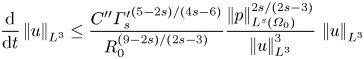
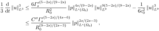 \begin{align} \frac{1}{3}\,\frac{\mathrm{d}}{\mathrm{d}t}\left|\mkern-2mu\left|u\right|\mkern-2mu\right|_{L^3}^3 &\le \frac{6{\varGamma_s'}^{(5-2s)/(9-2s)}}{R_0^2} \left|\mkern-2mu\left|p\right|\mkern-2mu\right|_{L^s(\varOmega_0)}^{4s/(9-2s)} \left|\mkern-2mu\left|u\right|\mkern-2mu\right|_{L^9}^{9(5-2s)/(9-2s)} - \frac{1}{6c_0^2}\left|\mkern-2mu\left|u\right|\mkern-2mu\right|_{L^9}^3 \nonumber\\ &\le \frac{C''{\varGamma_s'}^{(5-2s)/(4s-6)}}{R_0^{(9-2s)/(2s-3)}} \left|\mkern-2mu\left|p\right|\mkern-2mu\right|_{L^s(\varOmega_0)}^{2s/(2s-3)}, \end{align}
where Young's inequality, which is valid for  $s>3/2$, has been used. Here $C''$ depends on $s$ only. It follows that
 \begin{equation} \frac{\mathrm{d}}{\mathrm{d}t}\left|\mkern-2mu\left|u\right|\mkern-2mu\right|_{L^3} \le \frac{C''{\varGamma_s'}^{(5-2s)/(4s-6)}}{R_0^{(9-2s)/(2s-3)}}\frac{\left|\mkern-2mu\left|p\right|\mkern-2mu\right|_{L^s(\varOmega_0)}^{2s/(2s-3)}} {\left|\mkern-2mu\left|u\right|\mkern-2mu\right|_{L^3}^3}\,\left|\mkern-2mu\left|u\right|\mkern-2mu\right|_{L^3} \end{equation}
and we have the regularity criterion
 \begin{equation} \int_0^T \frac{{\varGamma_s'}^{(5-2s)/(4s-6)}}{R_0^{(9-2s)/(2s-3)}}\frac{\left|\mkern-2mu\left|p\right|\mkern-2mu\right|_{L^s(\varOmega_0)}^{2s/(2s-3)}} {\left|\mkern-2mu\left|u\right|\mkern-2mu\right|_{L^3}^3}\,\mathrm{d} t<\infty,\quad \mbox{for}\ s\in(3/2,9/4]. \end{equation}
Remark It can be seen that  $\varGamma _2'=\varGamma _7$. However, criterion (3.16) for $s=7$ and criterion (3.23) for $s=2$ are quite distinct.
Another family of regularity criteria can be deduced immediately from the evolution equation for  $\left |\mkern -2mu\left |u\right |\mkern -2mu\right |_{L^q}$. Indeed (3.14) implies that $\left |\mkern -2mu\left |u\right |\mkern -2mu\right |_{L^q}$ decays if
 \begin{equation} \int_{\varOmega_0}p^2|u|^{q-2}\, {\textrm{d} x} \le \frac{R_0^2}{4c_0^2q^2}\left|\mkern-2mu\left|u\right|\mkern-2mu\right|_{L^{3q}}^q. \end{equation}
This raw, unprocessed result seems to be the strongest here and its plausibility can be readily examinable. The case  $q=3$ is of special interest, which is treated in more detail in § 4. For this case, we start from (3.1), slightly decrease $U$, say
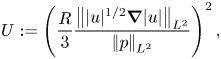 \begin{equation} U := \left(\frac{R}{3}\frac{\left|\mkern-2mu\left||u|^{1/2}\boldsymbol{\nabla}|u|\right|\mkern-2mu\right|_{L^2}}{\left|\mkern-2mu\left|p\right|\mkern-2mu\right|_{L^2}}\right)^2, \end{equation}
ignore the reduction of the driving set from  $\varOmega$ to $\varOmega _0$ and a ratio similar to $R_0$ and obtain the criterion
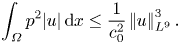 \begin{equation} \int_{\varOmega}p^2|u|\, {\textrm{d} x} \le \frac{1}{c_0^2}\left|\mkern-2mu\left|u\right|\mkern-2mu\right|_{L^9}^3. \end{equation}
In comparison with (3.24), there is clear gain here by a factor of  $32$, but with some loss due to the fact that $\varOmega _0\subseteq \varOmega$ (and $\varOmega$ is slightly larger than its original counterpart due to the decrease in $U$).
$U$).
4. Further estimates
This section examines a feature in the driving term of the evolution equation for  $\left |\mkern -2mu\left |u\right |\mkern -2mu\right |_{L^q}$ that can improve the results presented in § 3. We discuss the plausibility of the derived criteria. It is argued that singularity via the critical scaling $|u(x)|\sim 1/|x-x'_0|$ may not be realisable.
4.1. Pressure moderation
In a neighbourhood of a local velocity maximum, such as the set  $\varOmega$ presently considered, the integrand $p|u|^{q-2}\,\hat {u}\boldsymbol {\cdot }\boldsymbol {\nabla }|u|$ of the integral driving the evolution of $\left |\mkern -2mu\left |u\right |\mkern -2mu\right |_{L^q}$ is not sign definite. Indeed, for $p<0$, along a streamline $\ell$ within $\varOmega$, $p|u|^{q-2}\,\hat {u}\boldsymbol {\cdot }\boldsymbol {\nabla }|u|<0$ when $\hat {u}\boldsymbol {\cdot }\boldsymbol {\nabla }|u|>0$ (upstream portion of $\ell$ up to the point where $\hat {u}\boldsymbol {\cdot }\boldsymbol {\nabla }|u|=0$) and $p|u|^{q-2}\,\hat {u}\boldsymbol {\cdot }\boldsymbol {\nabla }|u|>0$ when $\hat {u}\boldsymbol {\cdot }\boldsymbol {\nabla }|u|<0$ (downstream portion of $\ell$). As a result, some partial cancellation takes place in the driving term. One may appreciate the significance of this cancellation by considering the case in which a local velocity maximum coincides with a local pressure minimum, whereby the fluid particle with the maximum velocity has zero acceleration. This may be called the case of ‘maximal’ cancellation. In order to exploit (and not to lose) this favourable feature, Tran & Yu (Reference Tran and Yu2016, Reference Tran and Yu2018, Reference Tran and Yu2019) have replaced the physical pressure $p$ in (2.2) by an effective pressure $\mathcal {P}$. Here we consider the version of $\mathcal {P}$ in Tran & Yu (Reference Tran and Yu2019). Let $f(x)$ be differentiable and $g(v)$, where $v\ge 0$, be locally integrable. Furthermore assume that $u\boldsymbol {\cdot }\boldsymbol {\nabla } f=0$. Now let $H(\sigma )$ be defined by
 \begin{equation} H(\sigma) := \int_0^\sigma g(v)v^q\,\mathrm{d}v, \end{equation}
for  $\sigma \in [0,\left |\mkern -2mu\left |u\right |\mkern -2mu\right |_{L^\infty }]$. Then $H(|u|)$ is differentiable and we have
 \begin{equation} fu\boldsymbol{\cdot}\boldsymbol{\nabla} H(|u|) = fg(|u|)|u|^qu\boldsymbol{\cdot}\boldsymbol{\nabla}|u|. \end{equation}
Integrating the above equation, noting that  $u\boldsymbol {\cdot }\boldsymbol {\nabla } f=0$ and $\boldsymbol {\nabla }\boldsymbol {\cdot } u=0$, yields
 \begin{equation} \int_{\mathbb{R}^3}fg|u|^qu\boldsymbol{\cdot}\boldsymbol{\nabla}|u|\,{\textrm{d} x} = 0. \end{equation}
Replacing  $p$ in (2.2) by $\mathcal {P}:=p+fg$ yields
 \begin{equation} \frac{1}{q}\,\frac{\mathrm{d}}{\mathrm{d}t}\left|\mkern-2mu\left|u\right|\mkern-2mu\right|_{L^q}^q \le (q-2)\int_{\mathbb{R}^3}\mathcal{P}|u|^{q-2}\hat{u}\boldsymbol{\cdot}\boldsymbol{\nabla}|u|\,{\textrm{d} x} - (q-1)\left|\mkern-2mu\left||u|^{(q-2)/2}\boldsymbol{\nabla}|u|\right|\mkern-2mu\right|_{L^2}^2. \end{equation}
 We set  $g(v)=0$ for $v\le U$ while $g(v)$ for $v>U$ is unspecified for now, where $U$ has been defined earlier in § 3. This means that $\mathcal {P}=p+fg$ in $\varOmega$ while $\mathcal {P}=p$ in $\varOmega ^c$ and $U$ and $\varOmega$ remain unchanged. In essence the physical pressure in $\varOmega$ is ‘moderated’ by the ‘moderator’ $fg$. Equations (3.1), (3.4) and (3.11) and all subsequent derivations and results remain valid with $p$ replaced by $\mathcal {P}$.
We assume that  $\varOmega$ is a simple set (or comprises a finite number of such sets). Figure 2 illustrates $\varOmega$ and its constituents $\varOmega '$ and $\varOmega _0$. Let $S\subset \varOmega$ denote the surface on which $|u|$ achieves a maximum along each streamline $\ell$, i.e. $\hat {u}\boldsymbol {\cdot }\boldsymbol {\nabla }|u|=0$ on $S$. On each $\ell$ within $\varOmega$, we set $f=-p(x'_0)$ and $g=1$, where $x'_0 := S\cap \ell$ (the coordinates of the streamline), so that $\mathcal {P}(x'_0)=0$. This choice of $f(x)$ satisfies the requirement $u\boldsymbol {\cdot }\boldsymbol {\nabla } f=0$ and ensures that $|u|$ and $|\mathcal {P}|$ are anti-correlated in the usual sense (peak $|u|$ coupled with vanishing $|\mathcal {P}|$), not only in $\varOmega$ but also on each streamline within $\varOmega$. Intuitively, replacing $p$ by $\mathcal {P}$ improves $\varGamma _q$ and all results derived thus far.
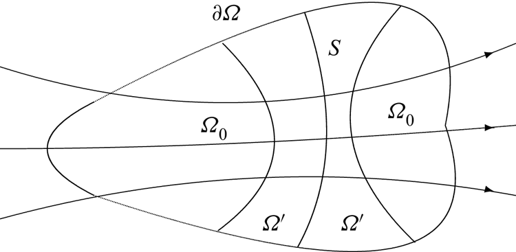
Figure 2. A schematic description of the high-velocity region  $\varOmega$, with boundary $\partial \varOmega$, and its constituents. The directed curves represent streamlines and $S\subset \varOmega$ is the surface where $u\boldsymbol {\cdot }\boldsymbol {\nabla }|u|=0$. Also on $S$, the effective pressure $\mathcal {P}=0$ for a simple pressure moderation scheme. That is on each streamline maximum $|u|$ is coupled with minimum $|\mathcal {P}|$. The set $\varOmega '$ (region of greatest velocity and smallest effective pressure $|\mathcal {P}|$) embraces $S$, and $\varOmega _0$ consists of two separated pieces on the sides of $\varOmega '$. The case of interest here is that the physical pressure p is lower downstream, so that high-velocity fluid on $S$ is accelerated.
There is a simple pressure moderation scheme, which is particularly effective when  $|u|$ and $|p|$ can be approximated by spherically symmetric functions like $\phi$ and $\psi$. Indeed, let $f(x)=-p(x'_0)/|u(x'_0)|^2$ and $g(|u|)=|u|^2$, so that $\mathcal {P}(x)$ be given by
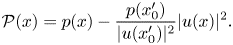 \begin{equation} \mathcal{P}(x) = p(x) - \frac{p(x'_0)}{|u(x'_0)|^2}|u(x)|^2. \end{equation}
Clearly  $\mathcal {P}(x'_0)=0$. Now if $|u(x)|$ and $p(x)$ are spherically symmetric about their peaks and can be approximated by $\phi$ and $\psi$, respectively, then $\mathcal {P}(x)\approx 0$ for perfect velocity–pressure correlation. Hence for this case, it seems plausible that $\varGamma _q$ becomes vanishingly small in the limit of perfect velocity–pressure correlation (perfect $|u|$– $|\mathcal {P}|$ anti-correlation). Thus, the extent of the improvement discussed in the preceding paragraph can be enormous.
4.2. The critical scaling
We now examine the plausibility of the criteria, particularly (3.26), presented in § 3 for flows with finitely many point singularities blowing up with the profile  $|x|^{-1}$. As is well known by the classical result of Caffarelli, Kohn & Nirenberg (Reference Caffarelli, Kohn and Nirenberg1982) (also see Lin (Reference Lin1998) and Robinson & Sadowski (Reference Robinson and Sadowski2012) and references therein), the parabolic Hausdorff dimension of alleged singular sets in space–time is strictly less than one. Consequently $|u|$ cannot blow up over a line segment of positive length. Furthermore, due to the scaling invariance of the Navier–Stokes system, a point blow-up with some local self-similarity should behave like $|x|^{-1}$. Note that although the blow-up of globally self-similar solutions has been disproved by Nečas, Røužicčka & Šverák (Reference Nečas, Røužicčka and Šverák1996), the possibility of solutions with local growth ${\sim }|x|^{-1}$, which may not be strictly self-similar, has not been ruled out. In fact, such solutions belong to the weak $L^3$ space, a slightly larger space than $L^3$, and it is not known whether solutions with uniform weak $L^3$ bounds remain globally smooth. In any case, Choe et al. (Reference Choe, Wolf and Yang2020) have recently proved that such solutions would become singular at (at most) finitely many points at the first singularity time. In what follows we work through some qualitative calculations for flows with this particular type of singular behaviour. More precisely, we assume that $\varOmega$ can be covered by finitely many balls, within each of which $|u|$ and $|p|$ can be approximated by $\phi$ and $\psi$ from (2.5a,b), respectively.
We recall the profiles of  $\phi$ and $\psi$ as defined in (2.5a,b), with $\alpha =1$, and identify $|u|$ with $\phi$, $|p|$ with $\psi$ and $\varOmega$ (and $\varOmega _0$) with $B(x_0,\delta )$. In essence, we assume $\varOmega \subset B(x_0,\delta )$, $|u|\approx \phi$ and $|p|\approx \psi$ in $B(x_0,\delta )$. As $\phi$ and $\psi$ are a priori singular while $u$ and $p$ are regular before the alleged singularity time $t=T_*$, this identification requires the following minor modification. Let $B(x_0,\epsilon _0)$, where $\epsilon _0\le \epsilon$, be embedded in $B(x_0,\epsilon )$, with the understanding that $\epsilon _0\to 0$ as $t\to T_*$. We regularise $p$ by setting $|p|\approx \epsilon _0^{-2}$ within $B(x_0,\epsilon _0)$ while still letting $|p|\approx \psi$ in the punctured ball $B^0(x_0,\delta ):=B(x_0,\epsilon )\setminus B(x_0,\epsilon _0)$. As will be seen shortly, it is not necessary to regularise $u$ in the estimation of mixed norms of $u$ and $p$. Now note that $B(x_0,\delta )$ and $B(x'_0,\delta )$ become indistinguishable in the limit $\epsilon _0\le \epsilon \to 0$. Hence while we use $B^0(x_0,\delta )$ and $B(x_0,\epsilon _0)$ in the estimation of mixed norms of $u$ and $p$, we use $B^0(x'_0,\delta ):=B(x'_0,\delta )\setminus B(x'_0,\epsilon _0)$ and $B(x'_0,\epsilon _0)$ in the estimation of pure norms of $u$. In this case, we regularise $u$ by setting $|u|\approx \epsilon _0^{-1}$ in $B(x'_0,\epsilon _0)$.
The coefficient  $\varGamma _3$ can be readily evaluated with the above approximations and the steps go as follows:
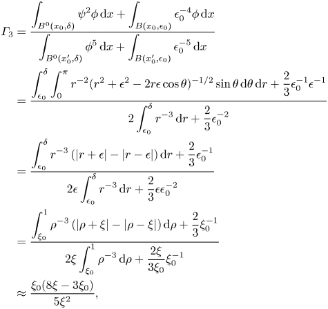 \begin{align} \displaystyle \varGamma_3&= \dfrac{\displaystyle\int_{B^0(x_0,\delta)}\psi^2 \phi\, {\textrm{d} x} +\int_{B(x_0,\epsilon_0)}\epsilon_0^{-4}\phi\,{\textrm{d} x}}{\displaystyle\int_{B^0(x_0',\delta)}\phi^5 \, {\textrm{d} x} +\int_{B(x_0',\epsilon_0)}\epsilon_0^{-5} \,{\textrm{d} x} }\nonumber\\ &= \dfrac{\displaystyle\int_{\epsilon_0}^\delta\int_0^{\rm \pi} r^{-2}(r^2+\epsilon^2-2r\epsilon\cos\theta)^{-1/2} \sin\theta\,\mathrm{d} \theta\,{\mathrm{d}} r + \dfrac{2}{3}\epsilon_0^{-1} \epsilon^{-1}}{\displaystyle2\int_{\epsilon_0}^\delta r^{-3}\,\mathrm{d} r + \dfrac{2}{3}\epsilon_0^{-2}}\nonumber\\ &= \dfrac{\displaystyle\int_{\epsilon_0}^\delta r^{-3}\left(|r+\epsilon|-|r-\epsilon|\right)\mathrm{d} r + \dfrac{2}{3}\epsilon_0^{-1}} {\displaystyle2\epsilon\int_{\epsilon_0}^\delta r^{-3}\,\mathrm{d} r+\dfrac{2}{3}\epsilon \epsilon_0^{-2}}\nonumber\\ &= \dfrac{\displaystyle\int_{\xi_0}^1 \rho^{-3}\left(|\rho+\xi|-|\rho-\xi|\right)\mathrm{d}\rho +\dfrac{2}{3}\xi_0^{-1}} {\displaystyle2\xi\int_{\xi_0}^1 \rho^{-3}\,\mathrm{d}\rho+\dfrac{2\xi}{3\xi_0}\xi_0^{-1}}\nonumber\\ &\approx \dfrac{\displaystyle\xi_0(8\xi-3\xi_0)}{5\xi^2}, \end{align}
where, again,  $\xi :=\epsilon /\delta$ while $\xi _0:=\epsilon _0/\delta$. Note that in the final step we only keep the leading-order contributions. It is clear that $\varGamma _3$ is an increasing function of $\xi _0$, achieving a maximum of one at $\xi _0=\xi$ (for a priori perfect correlation). An important implication of (4.6) is that in the limit of perfect correlation, $\varGamma _3$ vanishes as $\xi _0/\xi \to 0$. The interpretation is that if the growth rate of $\left |\mkern -2mu\left |u\right |\mkern -2mu\right |_{L^\infty }$ (represented by $\xi _0\to 0$) outperforms that of the degree of velocity–pressure correlation (represented by $\xi \to 0$), then $\varGamma _3\to 0$.
We now estimate the ratio  $\int _{\varOmega }p^2|u|\,{\textrm {d} x}/\left |\mkern -2mu\left |u\right |\mkern -2mu\right |_{L^9}^3$ and compare the result with $1/c_0^2=3/(2/{\rm \pi} )^{4/3}$ for a sense of the plausibility of criterion (3.26). Similar to (4.6) we have
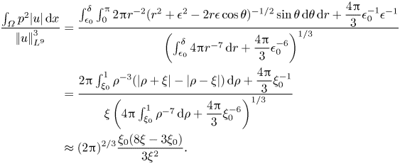 \begin{align} \frac{\int_{\varOmega}p^2|u|\,{\textrm{d} x}}{\left|\mkern-2mu\left|u\right|\mkern-2mu\right|_{L^9}^3} &= \dfrac{\int_{\epsilon_0}^\delta\int_0^{\rm \pi}2{\rm \pi} r^{-2} (r^2+\epsilon^2-2r\epsilon\cos\theta)^{-1/2}\sin\theta\,\mathrm{d} \theta\,\mathrm{d} r + \dfrac{4{\rm \pi} }{3}\epsilon_0^{-1}\epsilon^{-1} } {\left(\int_{\epsilon_0}^\delta 4{\rm \pi} r^{-7}\,\mathrm{d} r +\dfrac{4{\rm \pi}}{3} \epsilon_0^{-6}\right)^{1/3}} \nonumber\\ &= \frac{2{\rm \pi}\int_{\xi_0}^1\rho^{-3}(|\rho+\xi|-|\rho-\xi|)\,\mathrm{d}\rho+ \dfrac{4{\rm \pi}}{3}\xi_0^{-1}} {\xi\left(4{\rm \pi}\int_{\xi_0}^1\rho^{-7}\,\mathrm{d}\rho +\dfrac{4{\rm \pi}}{3}\xi_0^{-6}\right)^{1/3}} \nonumber\\ &\approx (2{\rm \pi})^{2/3}\frac{\xi_0(8\xi-3\xi_0)}{3\xi^2}. \end{align}
Hence, criterion (3.26) holds and  $\left |\mkern -2mu\left |u\right |\mkern -2mu\right |_{L^3}$ decays if
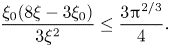 \begin{equation} \frac{\xi_0(8\xi-3\xi_0)}{3\xi^2} \le \frac{3{\rm \pi}^{2/3}}{4}. \end{equation}
We are primarily interested in the situation where  $|u|$ and $p$ are not a priori perfectly correlated, i.e. $\xi >0$. In this case we may, without loss of generality, impose an upper bound (arbitrarily small) on the ratio $\xi _0/\xi$. By setting this bound slightly less than one, we see that (4.8) holds. This means that viscous forces have an edge over their nonlinear counterparts if $|u|$ and $|p|$ obey the critical scalings. Now, if we factor in the effect of pressure moderation, i.e. replacing $p$ by $\mathcal {P}$, then an improvement would mean that viscous forces overwhelm those of nonlinearity. Note that (4.8) does not depend explicitly on the growth rate of $\left |\mkern -2mu\left |u\right |\mkern -2mu\right |_{L^3}$. For the critical scaling under the present consideration, one may expect $\left |\mkern -2mu\left |u\right |\mkern -2mu\right |_{L^3}$ to have a temporal dependence of the form $\left |\mkern -2mu\left |u\right |\mkern -2mu\right |_{L^3}\approx (\log 1/\xi _0)^{1/3}\approx (\log 1/(T_*-t))^{1/3}$ near the alleged singularity time $T_*$. This satisfies the singularity criterion (1.5), yet (4.8) suggests no blow-up.
Finally, we consider  $1<\alpha <3/2$ but require $\epsilon >0$ in the definition of $\phi$ and $\psi$ in § 2. The upper bound $\alpha <3/2$ is to ensure that $\phi \in L^2(B)$, just like $u\in L^2(\mathbb {R}^3)$. It is straightforward to verify that $\chi :=\phi ^{1/2}\psi ^{1/4}\in L^4(B)$. Now by the Cauchy–Schwarz and Calderón–Zygmund inequalities we have
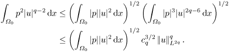 \begin{align} \int_{\varOmega_0}p^2|u|^{q-2}\,{\textrm{d} x} &\le \left(\int_{\varOmega_0}|p||u|^2\,{\textrm{d} x}\right)^{1/2} \left(\int_{\varOmega_0}|p|^3|u|^{2q-6}\,{\textrm{d} x}\right)^{1/2} \nonumber\\ &\le \left(\int_{\varOmega_0}|p||u|^2\,{\textrm{d} x}\right)^{1/2} c_q^{3/2}\left|\mkern-2mu\left|u\right|\mkern-2mu\right|_{L^{2q}}^q. \end{align}
It follows that criterion (3.24) holds and  $\left |\mkern -2mu\left |u\right |\mkern -2mu\right |_{L^q}$ decays if
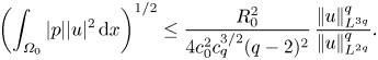 \begin{equation} \displaystyle \left(\int_{\varOmega_0}|p||u|^2\,{\textrm{d} x}\right)^{1/2} \le \frac{R_0^2}{4c_0^2c_q^{3/2}(q-2)^2}\, \frac{\left|\mkern-2mu\left|u\right|\mkern-2mu\right|_{L^{3q}}^q}{\left|\mkern-2mu\left|u\right|\mkern-2mu\right|_{L^{2q}}^q}. \end{equation}
By identifying  $|p||u|^2$ with $\chi ^4$ and $\varOmega _0$ with $B$, we see that the left-hand side of (4.10) remains finite while the right-hand side (strongly) diverges in the limit of large $\left |\mkern -2mu\left |u\right |\mkern -2mu\right |_{L^{3q}}$. Hence (4.10) holds when $\left |\mkern -2mu\left |u\right |\mkern -2mu\right |_{L^{3q}}$ becomes sufficiently large, and singularity is ruled out. Note that pressure moderation is unnecessary in this case, where the velocity and pressure extrema are mutually exclusive.
5. Conclusion
We have studied the evolution equation for the velocity norm  $\left |\mkern -2mu\left |u\right |\mkern -2mu\right |_{L^q}$, where $q\ge 3$, in Navier–Stokes flows, with an emphasis on the effects of the spatial correlation between the velocity and pressure on the growth rate of $\left |\mkern -2mu\left |u\right |\mkern -2mu\right |_{L^q}$. When the term driving the evolution of $\left |\mkern -2mu\left |u\right |\mkern -2mu\right |_{L^q}$ in this equation does not exceed its dissipation counterpart, $\left |\mkern -2mu\left |u\right |\mkern -2mu\right |_{L^q}$ does not grow and regularity persists. This ‘raw’ regularity criterion is strongest in the sense that any results derived from it cannot render improvements.
It has been found that strong growth of  $\left |\mkern -2mu\left |u\right |\mkern -2mu\right |_{L^q}$ necessarily requires a high correlation between low pressure and high velocity. Furthermore, singularity requires a coalescence of the velocity maximum and pressure minimum in the final stage of their singular growth. This constraint is quite stringent as a priori alignment of these extrema means that the fluid particle with the maximum velocity resides at the centre of the pressure minimum and therefore does not accelerate, hence regularity persists.
We have considered the possibility of blow-up via the critical scaling of the Navier–Stokes system. It has been shown that  $u$ and $p$ may not become singular at $t=T_*$ in the manner $|u(x,t)|\to 1/|x-x'_0|$ and $|p(x,t)|\to 1/|x-x_0|^2$, in which $\epsilon (t):=|x_0(t)-x'_0(t)|\to 0$ as $t\to T_*$. This result does not depend on how $\epsilon (t)$ approaches zero. Here, $\epsilon$ represents a straightforward measure of the spatial correlation between $u$ and $p$ approximated by simple functions. In general, a more sophisticated measure of this correlation is desirable. We have considered a mathematical measure arising naturally from the evolution equation for $\left |\mkern -2mu\left |u\right |\mkern -2mu\right |_{L^q}$. Admittedly, the consideration falls short of a quantitative mathematical theory to address the regularity problem in a rigorous manner, beyond approximations of $u$ and $p$ by simple functions. Such a theory should desirably be dynamically bound, addressing local behaviour of the hybrid dynamical quantities $|u|^a|p|^b$ (or $|u|^a|\mathcal {P}|^b$), where $a,b>0$, and their various Lebesgue norms. A detailed understanding of $\left |\mkern -2mu\left ||u|^a|p|^b\right |\mkern -2mu\right |_{L^s}$ entails a firm knowledge of the correlation coefficient $\varGamma _q$ put forward in this work.
Intuitively, energetic fluid particles are optimally accelerated when progressively lower-pressure regions form in front of them, thereby guiding and driving them to progressively higher velocity, without encountering much viscous resistance. This seems to be a plausible scenario for singularity, but a mechanism underpinning the formation of such a continuous (and accelerating) chain of dynamic low-pressure regions appears to be non-existent. On the other hand, fluid particles can be accelerated towards a relatively static low-pressure region. For singularity, the pressure of the region must decrease to negative infinity, but the incoming incompressible fluid works against the maintenance of such a static region, let alone driving its pressure ever lower. Hence, it is inconceivable that a relatively static minimum pressure can become singular. In naive but informative terms, on the verge of singularity, the pre-singular low-pressure region ( $\varOmega$ or $\varOmega _0$ in the present study) would act as a black hole that is unable to accommodate any incoming material. Apparently, this is physically if not mathematically self-contradictory.
It is well known in fluid mechanics that the pressure achieves a local minimum at the centre of a vortex, where the vorticity is greatest but the velocity is low or moderate. This corresponds to high vorticity–pressure correlation but relatively low velocity–pressure correlation in the present sense. The former is consistent with the diagnostic equation
 \begin{equation} \Delta p = -\boldsymbol{\nabla}\boldsymbol{\cdot}(u\boldsymbol{\cdot}\boldsymbol{\nabla})u = |\boldsymbol{\nabla}\times u|^2 - |\boldsymbol{\nabla} u|^2, \end{equation}
where a minimum pressure requires relatively large vorticity  $|\boldsymbol {\nabla }\times u|$. It appears that (5.1), which is a direct consequence of the incompressibility condition, may shed some light on the compatibility between velocity maxima and pressure minima. If these extrema are mutually exclusive, then Navier–Stokes flows are regular.
Acknowledgements
We thank the editor and the anonymous referees for invaluable and insightful comments.
Funding
X.Y. is supported by an NSERC Discovery grant.
Declaration of interests
The authors report no conflict of interest.
Appendix A
This appendix presents a sketch of proof of the existence of  $\varOmega (t)$ (as well as $U$).
$U$).
Define  $\varOmega (s):=\{x\mid |u(x,t)|>s\}$ and $F(s):=\left |\mkern -2mu\left ||u|^{(q-2)/2}\boldsymbol {\nabla }|u|\right |\mkern -2mu\right |_{L^2(\varOmega (s)^c)}^{2/(q-2)}$, for $s\in (0,\infty )$. It can be seen that the existence of $s$ satisfying $s\ F(s) = \big(\left |\mkern -2mu\left ||u|^{(q-2)/2}\boldsymbol {\nabla }|u|\right |\mkern -2mu\right |_{L^2}^2/2\ |\mkern -2mu |p |\mkern -2mu |_{L^2}\big)^{2/(q-2)}$ entails the existence of $\varOmega (s)$. Now observe that $F(s)\to 0$ as $s\to 0$ and $F(s)\to \left |\mkern -2mu\left ||u|^{(q-2)/2}\nabla |u|\right |\mkern -2mu\right |_{L^2(\mathbb {R}^3)}^{2/(q-2)}>0$ as $s\to \infty$. We further claim that $F(s)$ is a continuous function, from which the desired existence of $s$ follows. To justify this claim, let $s_0\in (0,\infty )$ be arbitrary. It is clear that
 \begin{equation} \varOmega(s)\to \varOmega(s_0) \text{ when }s\to s_0 \quad\text{and}\quad \varOmega(s)\to \varOmega(s_0)\cup \varOmega_0 \text{ when }s\to s_0, \end{equation}
where  $\varOmega _0:=\{x\mid |u(x,t)|=s_0\}$. Continuity of $F(s)$ now follows from Lebesgue's dominated convergence theorem and the fact that $\boldsymbol {\nabla }|u|=0$ almost everywhere on $\varOmega _0$. A more detailed presentation of this step can be found in § 3 of Tran & Yu (Reference Tran and Yu2018).
Appendix B
This appendix presents a proof of theorem 3.1.
(a) Substituting (3.15) into (3.14), we obtain
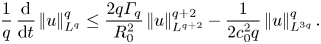 \begin{equation} \frac{1}{q}\,\frac{\mathrm{d}}{\mathrm{d}t}\left|\mkern-2mu\left|u\right|\mkern-2mu\right|_{L^q}^q \le \frac{2q\varGamma_q}{R_0^2}\left|\mkern-2mu\left|u\right|\mkern-2mu\right|_{L^{q+2}}^{q+2} - \frac{1}{2c_0^2q}\left|\mkern-2mu\left|u\right|\mkern-2mu\right|_{L^{3q}}^q. \end{equation}
By applying the interpolation inequality  $\left |\mkern -2mu\left |u\right |\mkern -2mu\right |_{L^{q+2}}^{q+2}\le \left |\mkern -2mu\left |u\right |\mkern -2mu\right |_{L^q}^{q-1}\left |\mkern -2mu\left |u\right |\mkern -2mu\right |_{L^{3q}}^3$ to the driving term in (B1) we obtain
 \begin{align} \frac{1}{q}\,\frac{\mathrm{d}}{\mathrm{d}t}\left|\mkern-2mu\left|u\right|\mkern-2mu\right|_{L^q}^q &\le \frac{2q\varGamma_q}{R_0^2}\left|\mkern-2mu\left|u\right|\mkern-2mu\right|_{L^q}^{q-1}\left|\mkern-2mu\left|u\right|\mkern-2mu\right|_{L^{3q}}^3 - \frac{1}{2c_0^2q}\left|\mkern-2mu\left|u\right|\mkern-2mu\right|_{L^{3q}}^q \nonumber\\ &\le C\left(\frac{\varGamma_q}{R_0^2}\right)^{q/(q-3)}\left|\mkern-2mu\left|u\right|\mkern-2mu\right|_{L^q}^{q(q-1)/(q-3)} \nonumber\\ &= C\left(\frac{\varGamma_q}{R_0^2}\right)^{q/(q-3)}\left|\mkern-2mu\left|u\right|\mkern-2mu\right|_{L^q}^{2q/(q-3)}\left|\mkern-2mu\left|u\right|\mkern-2mu\right|_{L^q}^q, \end{align}
where Young's inequality, which is valid for  $q>3$, has been used. Here $C$ depends on $q$ (and $c_0$) only. Integrating (B2) yields
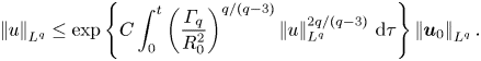 \begin{equation} \left|\mkern-2mu\left|u\right|\mkern-2mu\right|_{L^q} \le \exp\left\{C\int_0^t\left(\frac{\varGamma_q}{R_0^2}\right)^{q/(q-3)} \left|\mkern-2mu\left|u\right|\mkern-2mu\right|_{L^q}^{2q/(q-3)}\,\mathrm{d}\tau\right\}\left|\mkern-2mu\left|\boldsymbol{u}_0\right|\mkern-2mu\right|_{L^q}. \end{equation}
This result means that  $\left |\mkern -2mu\left |u\right |\mkern -2mu\right |_{L^q}$ is finite as long as the time integral on the right-hand side remains finite, hence criterion (3.16).
(b) For  $q=3$, (B1) becomes
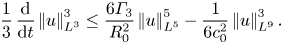 \begin{equation} \frac{1}{3}\,\frac{\mathrm{d}}{\mathrm{d} t}\left|\mkern-2mu\left|u\right|\mkern-2mu\right|_{L^3}^3 \le \frac{6\varGamma_3}{R_0^2}\left|\mkern-2mu\left|u\right|\mkern-2mu\right|_{L^5}^5 - \frac{1}{6c_0^2}\left|\mkern-2mu\left|u\right|\mkern-2mu\right|_{L^9}^3. \end{equation}
Following Tran & Yu (Reference Tran and Yu2017b), we use the interpolation inequality
 \begin{equation} \left|\mkern-2mu\left|u\right|\mkern-2mu\right|_{L^5}^5 \le \left|\mkern-2mu\left|u\right|\mkern-2mu\right|_{L^s}^{4s/(9-s)}\left|\mkern-2mu\left|u\right|\mkern-2mu\right|_{L^9}^{9(5-s)/(9-s)}, \end{equation}
for  $s\le 5$. Substituting this estimate into (B4) and invoking Young's inequality, which is valid for $s>3$, yield
 \begin{align} \frac{1}{3}\,\frac{\mathrm{d}}{\mathrm{d} t}\left|\mkern-2mu\left|u\right|\mkern-2mu\right|_{L^3}^3 &\le \frac{6\varGamma_3}{R_0^2}\left|\mkern-2mu\left|u\right|\mkern-2mu\right|_{L^s}^{4s/(9-s)}\left|\mkern-2mu\left|u\right|\mkern-2mu\right|_{L^9}^{9(5-s)/(9-s)} - \frac{1}{6c_0^2}\left|\mkern-2mu\left|u\right|\mkern-2mu\right|_{L^9}^3 \nonumber\\ &\le C'\left(\frac{\varGamma_3}{R_0^2}\right)^{(9-s)/(2s-6)}\left|\mkern-2mu\left|u\right|\mkern-2mu\right|_{L^s}^{2s/(s-3)}, \end{align}
where  $C'$ depends on $s$ only. It follows that
 \begin{equation} \frac{\mathrm{d}}{\mathrm{d} t}\left|\mkern-2mu\left|u\right|\mkern-2mu\right|_{L^3} \le C'\left(\frac{\varGamma_3}{R_0^2}\right)^{(9-s)/(2s-6)}\frac{\left|\mkern-2mu\left|u\right|\mkern-2mu\right|_{L^s}^{2s/(s-3)}}{\left|\mkern-2mu\left|u\right|\mkern-2mu\right|_{L^3}^3}\, \left|\mkern-2mu\left|u\right|\mkern-2mu\right|_{L^3}. \end{equation}
By integrating (B7) one immediately deduces criterion (3.17) after invoking the concluding argument in (a).
(c) Again following Tran & Yu (Reference Tran and Yu2017b) we apply the interpolation inequality
 \begin{equation} \left|\mkern-2mu\left|u\right|\mkern-2mu\right|_{L^5}^5 \le \left|\mkern-2mu\left|u\right|\mkern-2mu\right|_{L^3}^{3(s-5)/(s-3)}\left|\mkern-2mu\left|u\right|\mkern-2mu\right|_{L^s}^{2s/(s-3)} \end{equation}
to (B4) to obtain
 \begin{equation} \frac{1}{3}\,\frac{\mathrm{d}}{\mathrm{d} t}\left|\mkern-2mu\left|u\right|\mkern-2mu\right|_{L^3}^3 \le \frac{6\varGamma_3}{R_0^2}\left|\mkern-2mu\left|u\right|\mkern-2mu\right|_{L^3}^{3(s-5)/(s-3)}\left|\mkern-2mu\left|u\right|\mkern-2mu\right|_{L^s}^{2s/(s-3)} - \frac{1}{6c_0^2}\left|\mkern-2mu\left|u\right|\mkern-2mu\right|_{L^9}^3. \end{equation}
It follows that
 \begin{equation} \frac{\mathrm{d}}{\mathrm{d} t}\left|\mkern-2mu\left|u\right|\mkern-2mu\right|_{L^3} \le \frac{6\varGamma_3}{R_0^2}\frac{\left|\mkern-2mu\left|u\right|\mkern-2mu\right|_{L^s}^{2s/(s-3)}}{\left|\mkern-2mu\left|u\right|\mkern-2mu\right|_{L^3}^{6/(s-3)}}\, \left|\mkern-2mu\left|u\right|\mkern-2mu\right|_{L^3}, \end{equation}
which implies criterion (3.18) upon integration.


 Open access