2. Background and literature review

Major changes in food consumption patterns and shifts in composition of consumer diets have been a noteworthy phenomenon observed in many parts of the world in recent decades (Hovhannisyan and Devadoss, Reference Hovhannisyan and Devadoss2020; Hovhannisyan and Gould, Reference Hovhannisyan and Gould2011; Regmi, Reference Regmi2001; Sharma, Nguyen, and Grote, Reference Sharma, Nguyen and Grote2018). Some of the most important changes have been the increased consumer demand for organic, local, environmentally friendly, sustainable, and functional foods that offer benefits beyond basic nutrition (e.g., Kearney, Reference Kearney2010). Despite these commonalities in food consumption trends, transition in dietary patterns has been found to vary by country due mainly to economic, socio-demographic and cultural differences, as well as urbanization and trade liberalization policies (Kearney, Reference Kearney2010; Popkin, Adair, and Ng, Reference Popkin, Adair and Ng2012).

Similar to the rest of the world, Russia has not been immune to nutrition transition. However, several special drivers set the country apart from many other consumer markets, an important one of which is the transition from a centrally planned to a market economy. Prior to this transition, the bulk of the nation’s food supply was provided by large state collective farms that were guided by 5-year long centralized economic plans. These plans were determined by state planning commissions that followed a top-down approach to policy decisions, oftentimes with little regard for consumer tastes, preferences, and desires (Sachs and Woo, Reference Sachs and Woo1994). Given the lack of foreign-supplied alternatives, consumer food choices were heavily influenced by planners’ preferences, which sought to expand the production of high-value livestock and dairy products (Liefert, Lohmar, and Serova, Reference Liefert, Lohmar and Serova2003). Consequently, the initial years of post-transformation went hand-in-hand with increasing consumer sovereignty and saw a considerable decline in per capita consumption of meat and dairy products. Meanwhile, consumption of bread, potatoes, and other food staples remained relatively stable (Liefert and Swinnen, Reference Liefert and Swinnen2002).Footnote ³

Trade liberalization that was carried out as an integral part of the economic transition is widely thought to have further contributed to changing consumer diets (Liefert, Lohmar, and Serova, Reference Liefert, Lohmar and Serova2003). Specifically, free trade with the rest of the world revealed Russia’s competitive disadvantage in the production of a number of agricultural products, including livestock and related products. As a result, the share of foreign-supplied agricultural products in domestic consumption increased, and as imports continued to grow and Russian consumers became increasingly reliant on imported food products, the drop in the consumption of livestock and similar products were somewhat mitigated (Liefert, Reference Liefert2002). Finally, price liberalization brought by the economic transition led to prices outstripping consumer incomes, which consequently reduced real income. This further reinforced the changes in livestock and dairy consumption, given the relatively higher income elasticities of demand for these food products (Liefert, Lohmar, and Serova, Reference Liefert, Lohmar and Serova2003).

Evidence suggests that consumer food tastes and preferences have continued to evolve during the early 2000s and through modern-day Russia. For example, meat consumption bounced back after years of decline and eventually exceeded the Soviet-era levels when per capita meat consumption reached 75 kg in 2017 (Vorotnikov, Reference Vorotnikov2017). An even more important change may have been a compositional shift in meat consumption with poultry and pork having gained popularity in recent years, while beef consumption remained relatively stable (FAS/USDA, 2015). Recent years have also seen a considerable increase in fresh fruit and vegetable consumption, which has been occurring at an average annual rate of 4% (WorldFood Moscow, 2018a). As a result, per capita vegetable consumption reached 112 kg in 2016, with potato, the “almighty Russian crop” continuing to be the most widely consumed vegetable (Fresh Plaza, 2017). With a steady rise in disposable income, however, potatoes are expected to be slowly replaced by other food products that are perceived as normal goods by Russian consumers.

In contrast, per capita consumption of dairy products stagnated and eventually declined to 233.4 kg in 2016, with the decline amounting to 9 kg over 2013–2015 alone (Meatinfo, 2020). This change in dairy consumption may be partially due to various milk adulteration practices such as substituting palm oil for milk, which, according to some expert estimates, have been affecting a quarter of dairy production in Russia (Barsukova, Reference Barsukova2016). This creates important opportunities for Russia’s trade partners, given the sizable gap between the actual and recommended dairy consumption (i.e., 325 kg annually) and the fact that Russian consumers expressed willingness to increase their dairy consumption, provided that product quality improves (Dairy Global, 2019).

A final important group of food categories deserving scrutiny comprises bread, pastry, other bakery goods, and cereals. Despite their historical significance from the perspective of dietary composition, consumption of many of these products has been on a decline due in part to high caloric intake and resultant health issues (Harvard Medical School, 2015). Evidence also suggests that artisan and whole grain breads have become increasingly popular with younger consumers, who highly value food freshness and quality. As a result, artisan bread became a market leader in 2016 with a 32% market share (ITEFood&Drink, 2017). In addition to quality features, consumers have also shown growing interest in cereal products that are convenient to store and offer longer-shelf-life. This led to an 11% increase in demand for these products in 2014 alone (ITEFood&Drink, 2017).

Consumption changes immediately following the break-up of the command economy were clearly a result of consumer preferences taking precedence over planners’ preferences. Later changes, however, were in all likelihood driven by a combination of factors such as the economic growth in the mid-2000s, improved food accessibility and availability, and more recent food safety issues that altered consumer incomes, food prices, and tastes and preferences.Footnote ⁴ The series of recent economic sanctions imposed by Russia on a range of imported agricultural products from a number of western nations may have further contributed to changes in food consumption patterns through their effects on the availability, variety, and accessibility of food products in the country’s domestic markets (Liefert and Liefert, Reference Liefert and Liefert2015). Nevertheless, the extent to which these recent consumption changes are tied to shifting consumer tastes and preferences rather than being reflective of sheer consumer response to changing economic circumstances under stable preferences has not received adequate research interest. Previous studies have almost exclusively focused on estimating the structure of demand for various food products based on an implicit assumption of fixed and exogenously given consumer preferences, where consumption changes are fully attributed to consumer response to changing opportunity set (e.g., Burggraf et al., Reference Burggraf, Kuhn, Qi-ran, Teuber and Glauben2015; Elsner, Reference Elsner1999; Hovhannisyan and Shanoyan, Reference Hovhannisyan and Shanoyan2019; and Staudigel and Schröck, Reference Staudigel and Schröck2015). However, structural changes can have significant effects on food preferences, the omission of which can result in inaccurate price and income effects, ultimately leading to erroneous policy implications.

We fill this gap by conducting a formal analysis of structural food preference change in Russia by adopting an advanced demand model and by utilizing the best time series of provincial-level panel data available. More specifically, we follow a large strand of literature by adopting a parametric approach to the analysis of consumer tastes and preferences (Okrent and Alston, Reference Okrent and Alston2011). Earlier studies in this line of literature evaluated structural change in terms of the inconsistency of model parameters with restrictions stemming from consumer theory (e.g., Blanciforti, Green, and King, Reference Blanciforti, Green and King1986) or relied on a Chow-type test for assessing the stability of behavioral parameters (e.g., Chavas, Reference Chavas1983; Goodwin, Reference Goodwin1989; Menkhaus, Clair and Hallingbye, Reference Menkhaus, Clair and Hallingbye1985).

We follow the most recent studies that adopt a more direct approach, whereby the structural parameters underlying consumer preferences are allowed to vary according to a variety of time transition functions, tested for stability, with a finding of instability interpreted as evidence of preference change (e.g., Dong and Fuller, Reference Dong and Fuller2010; Hovhannisyan and Gould, Reference Hovhannisyan and Gould2014; Moschini, Moro, and Green, Reference Moschini, Moro and Green1994). In an empirical application of this framework to the analysis of food demand in China, for example, Hovhannisyan and Gould (Reference Hovhannisyan and Gould2014) found that consumers had undergone considerable preference changes in the recent years with meats and fruits replacing roots and tubers in the traditional Chinese food diet, while relatively older consumers with lower levels of educational attainment were found to be immune to these dietary transitions. However, these results need to be interpreted with caution as econometric issues such as price endogeneity were not addressed in the previous analyses. Our study, on the other hand, provides the first attempt at addressing food price endogeneity in a structural preference change context.

A nonparametric method represents an alternative way of analyzing consumer preference change that has been used extensively in the past literature. The essence of this approach consists in assessing the consistency of food consumption data in hand with the generalized (GARP), strong (SARP), and weak axioms of revealed preferences (WARP), with a finding of consistency interpreted as a lack of preference change (e.g., Bergtold, Akobundu, and Peterson, Reference Bergtold, Akobundu and Peterson2004; Brester and Schroeder, Reference Brester and Schroeder1995; Chalfant and Alston, Reference Chalfant and Alston1988). However, a major downside of this test has been found to be the lack of power in detecting preference change when aggregate data are utilized in the analyses, which may paradoxically lead to a conclusion of stable consumer preferences even when the actual reality is different (Okrent and Alston, Reference Okrent and Alston2011). Therefore, we confine our attention to the parametric methods that utilize a switching regression framework developed by Ohtani and Katayama (Reference Ohtani and Katayama1986) and popularized by a number of studies such as Moschini and Meilke (Reference Moschini and Meilke1989) and Dong and Fuller (Reference Dong and Fuller2010). This analytical framework allows for estimating potential change in structural parameters of the model by specifying all the possible permutations of starting and ending points of the change, thus allowing for the possibility of both abrupt and gradual change.

3. Methodology

In this section, we provide a brief discussion of the GEASI demand system underlying our empirical analysis. Next, we extend the GEASI via the incorporation of a time transition function that allows for evaluating structural food preference changes. Finally, we discuss price endogeneity and the resulting effects brought by the constant shifts of supply and demand curves, as well as present an identification strategy to address this econometric issue.

3.1. A Generalized Exact Affine Stone Index demand specification

Let ${w_i}$, ${p_i}$, and ${c_i}$denote the budget share, price, and pre-committed demand (i.e., invariant to income and price changes) for product i, respectively, X denote household total food and non-food expenditures, ${\varepsilon _i}$ reflect unobserved preference heterogeneity, and ${\alpha _{ik}}$, ${\beta _{ir}}$be parameters representing the price and income effects on demand. The GEASI demand model can then be represented by the following system of equations (Hovhannisyan and Shanoyan, Reference Hovhannisyan and Shanoyan2019):

(1)$${w_i} = {{{c_i}{p_i}} \over X} + \left( {1 - {{c'p} \over X}} \right)\left( {\sum\limits_{l = 0}^L {{\beta _{il}}} {{\left( {\ln \left( {X - c'p} \right) - w'\ln p} \right)}^l} + \sum\limits_{k = 1}^N {{\alpha _{ik}}\ln {p_k}} } \right) + {\varepsilon _i},\,\,\forall i = 1,...,N,$$

where $\left( {\ln \left( {X - c'p} \right) - w'\ln p} \right)$is price and pre-commitment (c)-adjusted total expenditure that captures the effects of real income; r denotes the order of the polynomial function of real income; $c'p$ represents pre-committed expenditures; and $\left( {X - c'p} \right)$ reflects supernumerary expendituresFootnote ⁵ that are driven by economic variables. The demand system in (1) is subject to the theoretical restrictions of adding-up $\sum\limits_{i = 1}^N {{\beta _{i0}} = 1;\,} \sum\limits_{i = 1}^N {{\beta _{il}} = 0,\,\forall l = 1,...,L;\sum\limits_{i = 1}^N {{\alpha _{ik}} = 0} } \,\left( {\forall k = 1,...,N} \right)$, and symmetry ${\alpha _{ik}} = {\alpha _{ki}}$$\left( {\,\forall i,k = 1,...,N} \right)$.

An important advantage of modeling pre-committed consumption that the GEASI provides is the more accurate estimation of price and income elasticities of demand. Specifically, elasticities measured in a given empirical setting reflect a summary estimate of consumer income and price responsiveness over both pre-committed and discretionary portions of a demand curve; thus, overlooking pre-committed quantities wrongly attributes consumer insensitivity to all consumption and results in less elastic estimates of economic effects (Rowland et al., Reference Rowland, Mjelde and Dharmasena2017).

3.2. A Generalized Exact Affine Stone Index-based analytical framework for structural preference change

We modify the GEASI model by introducing a time transition function that resembles a gradual switching regression and is adopted from Ohtani and Katayama (Reference Ohtani and Katayama1986):

$${h_t} = 0,\,\,\,\,\,{\rm{for}}\,\,\,\,\,t = 1,...,{\tau _1}$$

(2)$${h_t} = \frac{{{\left( {t - {\tau _1}} \right)}}\over{{\left( {t - {\tau _2}} \right)}}},\,\,\,\,\,{\rm{for}}\,\,\,\,\,t = {\tau _1} + 1,...,{\tau _2} - 1$$

$${h_t} = 1,\,\,\,\,\,{\rm{for}}\,\,\,\,\,t = {\tau _2},...,T,$$

where ${\tau _1}$denotes the end of the first regime, and ${\tau _2}$ indicates the beginning of the second regime (i.e., ${\tau _1}$<${\tau _2}$), and the period between ${\tau _1}$ and ${\tau _2}$captures the transition path (i.e., ${\tau _1} + 1$ = ${\tau _2}$ is indicative of an abrupt change, whereas ${\tau _1} + 1$<${\tau _2}$is interpreted as gradual transition).

Incorporation of the time transition function in equation (2) into the GEASI system in equation (1) generates the following model that allows for the evaluation of preference change:Footnote ⁶

(3)$${w_{irt}} = {{c_i^h{p_{irt}}} \over {{X_{rt}}}} + \left( {1 - {\rm{ }}{{{c^h}^\prime p} \over {{X_{rt}}}}} \right)\left( {\sum\limits_{l = 0}^L {\beta _{il}^h} {{\left( {\ln \left( {{X_{rt}} - {c^h}^\prime p} \right) - w'\ln p} \right)}^l} + \sum\limits_{k = 1}^N {\alpha _{ik}^h\ln {p_{krt}}} } \right) + {\xi _{irt}},$$

where $c_i^h = {c_{i0}} + c_{i1}^h{h_t}$, $\beta _{il}^h = {\beta _{il0}} + \beta _{il1}^h{h_t}$, $\alpha _{ik}^h = {\alpha _{ik0}} + \alpha _{ik1}^h{h_t}$; and $\sum\limits_{i = 1}^N {\beta _{il1}^h = 0;\,} \forall l = 1,...,L$, $\sum\limits_{i = 1}^N {\alpha _{ik1}^h = 0,\,\forall k = 1,...,N} $ present an additional set of restrictions to be imposed on the system.

Finally, we adjust the elasticity formulas derived by Hovhannisyan and Shanoyan (Reference Hovhannisyan and Shanoyan2019) to reflect the underlying demand specification in equation (3) and to allow for the assessment of potential structural parameter change.

3.3. Price endogeneity and the identification strategy

An important distinguishing characteristic of agricultural production is its exposure to disease, weather, climate, and natural calamities, which usually generate large swings in the supply of food commodities. When combined with the inelastic food demand, supply instability can generate considerable price variability in agriculture. Evidence suggests that these unpredictable supply forces are indeed some of the most important drivers behind agricultural price volatility (Gilbert, Reference Gilbert2010). Despite this reality, literature on food demand in Russia has overlooked this particular source of price variation because of limited data, thus relying only on demand factors for the identification of structural demand parameters (Shiptsova, Goodwin, and Holcomb, Reference Shiptsova, Goodwin and Holcomb2004; Staudigel, and Schröck, Reference Staudigel and Schröck2015). This creates an endogeneity bias given that the error terms in the commodity demand equations reflect both unobserved demand and supply effects and can generate inconsistent parameter estimates and economic effects, ultimately leading to erroneous policy recommendations (Hovhannisyan and Bozic, Reference Hovhannisyan and Bozic2017). For example, the recent expansion in the Russian grain, pork, and poultry production driven by the country’s desire for self-sufficiency in light of the recent developments in the global trade protectionism may be wrongly attributed to growing demand for these products and not the push from the government to expand these industries. Similarly, drought-induced feed price spikes and resulting beef cow herd liquidation may create an impression of structural changes in consumer tastes and preferences, when no such changes are present.

To address price endogeneity, we follow Dhar, Chavas, and Gould (Reference Dhar, Chavas and Gould2003) to supplement our demand system by reduced-form supply equations. These equations express food commodity prices in terms of exogenous supply determinants such as temperature, rainfall, and pollution,Footnote ⁷ thus making it possible to disentangle the simultaneous effects of demand and supply forces on agricultural prices and quantities, as presented below:Footnote ⁸

(4)$$\ln \left( {{p_{irt}}} \right) = {\mu _{i0}} + {\mu _{i1}}{\rm{RF}}\_{{\rm{1}}_{rt}} + {\mu _{i2}}{\rm{RF}}\_{{\rm{2}}_{rt}} + {\mu _{i3}}{\rm{TP}}\_{{\rm{1}}_{rt}} + {\mu _{i4}}{\rm{TP}}\_{{\rm{2}}_{rt}} + {\mkern 1mu} {\mu _{i5}}{\rm{GS}}{{\rm{E}}_{rt}} + {\mu _{i6}}{\rm{P}}{{\rm{W}}_{rt}}{\mkern 1mu} {\mkern 1mu} {\mkern 1mu} {\mkern 1mu} + {\rm{ }}{\mu _{i7}}{\rm{ALP}}{{\rm{C}}_{rt}} + {\mu _{i8}}{\rm{F}}{{\rm{W}}_{rt}} + {\rm{ }}{\varsigma _{irt}},\;\forall i = 1,...,{\mkern 1mu} N;{\mkern 1mu} {\mkern 1mu} r = 1,...,R;{\mkern 1mu} {\mkern 1mu} t = 1,...,T.$$

where ${\rm{RF\_}}{{\rm{1}}_{rt}}$ and ${\rm{RF\_}}{{\rm{2}}_{rt}}$measure January and July rainfall in region r in year t (mm),${\rm{TP\_}}{{\rm{1}}_{rt}}$ and ${\rm{TP\_}}{{\rm{2}}_{rt}}$ denote January and July temperatures in region r in year t (°C), respectively, ${\rm{GS}}{{\rm{E}}_{rt}}$ denotes the amount of gas emitted (1,000 metric tons), ${\rm{P}}{{\rm{W}}_{rt}}$ represents the amount of polluted water used in region r in year t (million ${m^3}$), ${\rm{ALP}}{{\rm{C}}_{rt}}$ reflects agricultural land per rural resident (1,000 ha), ${\rm{F}}{{\rm{W}}_{rt}}$ measures the amount of freshwater used in agricultural production (million ${m^3}$), ${\varsigma _{irt}}$ is the residual of the ${i^{th}}$ reduced-form supply equation, and ${\mu _{i0}}$–${\mu _{i8}}$ are parameters.

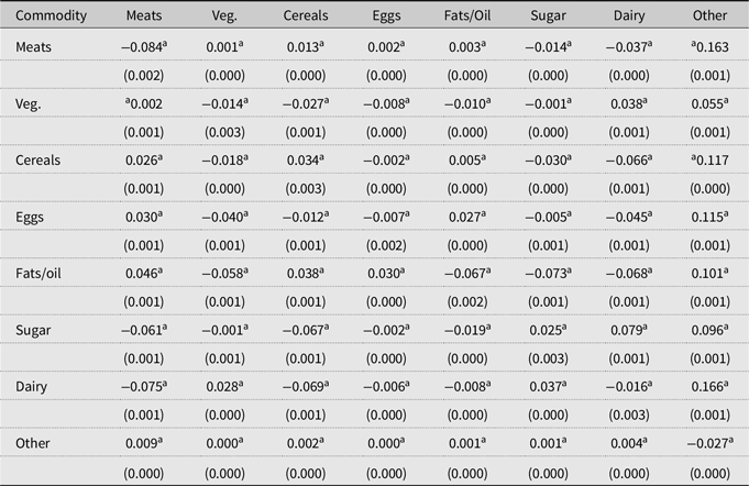
The agricultural commodity supply determinants utilized in this study are expected to affect prices through their influence on commodity stocks (Headey and Fan, Reference Headey and Fan2008). For example, extremely high temperatures and lack of rainfall can lead to an unfavorable impact on crop yields and food supply, thus generating upward pressure on prices, ceteris paribus. Similarly, expanding agricultural land base can lead to crop production growth and subsequent downward pressure on agricultural prices. Therefore, we anticipate that our supply shifters satisfy the instrument relevance condition. Additionally, our supply factors, especially the ones related to weather, climate, and pollution, reflect unforeseeable supply shocks that are properly excluded from commodity demand equations and are distinct from unobserved demand determinants, thus satisfying the instrument exogeneity requirement.

4. Provincial-level food consumption data

Our empirical application is based on provincial-level food consumption data obtained from the Federal State Statistics Service (FSSS) of Russia. The FSSS compiles information regarding household income, food consumption, expenditures, consumer socio-economic and demographic characteristics, as well as agricultural production and other related aspects of Russian households using a representative sample of consumers from more than 70 administrative divisions (e.g., oblasts and autonomous republics). Quarterly surveys are conducted within the framework of the Household Income and Food Expenditure Survey based on a two-stage stratified systematic random sampling method. Specifically, a third of the households sampled are dropped each period and replaced with a new sample of the same size using a rotating-sample design. The household-level data are subsequently aggregated by the FSSS to the administrative division level, and from quarterly to annual level before the data are made publicly available (Hovhannisyan and Shanoyan, Reference Hovhannisyan and Shanoyan2019).

In the current study, we confine our analysis to the consumer demand structure for seven food commodity aggregates, namely meats, vegetables, cereals, eggs, vegetable oils, sugar, and dairy, which we supplement by a composite numéraire good to account for the consumption of other food and non-food goods (denoted by “other”). Our choice of this approach reflects its advantage in sidestepping potential undesirable consequences of two-stage budgeting or separability assumptions that have been used widely in previous literature (e.g., Moschini, Moro, and Green, Reference Moschini, Moro and Green1994; Zhen et al., Reference Zhen, Finkelstein, Nonnemaker, Karns and Todd2013). Categorizing the seven commodity groups and numéraire good generates 5,896 total observations over 11 years (i.e., 2006–2016) and across 67 regions. We limit our empirical analysis to 67 regions/administrative units (mainly called oblasts) due to limited data on price instruments from the remaining regions. Online supplementary appendix presents all the regions comprising Russia, meanwhile highlighting the ones underlying the current study.

As can be seen from the descriptive statistics presented in Table 1, food expenditures continue to make up an important share of consumer income in Russia. Specifically, meats, cereals, dairy, vegetables, sugar, eggs, and vegetable oils collectively account for 47.8% of income, while the remaining 52.1% is allocated to other food and non-food items purchased by a typical Russian consumer. Using commodity expenditures and the respective consumption amounts, we further compute commodity unit values as proxies for food category prices.

Table 1. Descriptive statistics

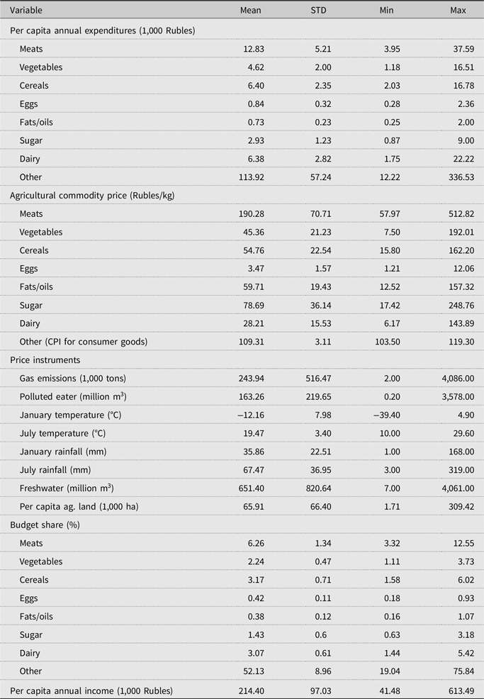
Source: Federal State Statistics Service of Russian Federation, 2006–2016.

Table 1 also provides descriptive statistics for a variety of weather-related variables and those reflecting agricultural production capacity that have been utilized in the demand system estimation to address food price endogeneity resulting from the simultaneous determination of supply and demand. These instruments manifest considerable spatial variation across the Russian regions, which is essential from the identification perspective. For example, agricultural land availability ranges from as low as 1.7 ha per rural resident in Murmansk to as high as 309.4 ha in Saratov. Similarly, greenhouse gas emissions extend from two thousand tons in Kabardino-Balkaria to 4,086 thousand tons in Tyumen, where the majority of oil and gas reserves and processing industries are concentrated. Due in part to this reason, Tyumen is also responsible for the highest amount (4,061 million m³) of freshwater use, while annual average freshwater consumption in Altai barely reached seven million m³. Additionally, we utilize data on polluted water in an attempt to account for the potential adverse effects of deteriorating water quality on agricultural production and commodity prices. Similar to other price instruments, water pollution appears to vary appreciably from 0.2 million m³ in the Altai Republic to 3,578 million m³ in Perm. Finally, Russian climate is continental and characterized by dry warm/hot summers (June temperature is 29.6°C in Samara) to cold winters (January temperature is −39.4°C in Yakutia), given the high latitude of the country (i.e., 40–75°N), with considerable provincial heterogeneity in terms of precipitation (e.g., 1–168 mm in January for Primorsk and Kaliningrad, respectively, and 3–319 mm in June for Astrakhan and Primorsk, respectively).

To explore the possibility of food preference change in Russia, as well as to shed light on the directions of potential dietary transition, we utilize spatial and temporal analyses of food consumption and income. As a first step, we perform a simple comparison of consumption of select food commodities (i.e., dairy, meat, and vegetables) in years 2006 and 2016. Specifically, vegetable consumption has undergone the most impressive change in this 11-year span, with almost all the provinces considered experiencing a sizable rise in the consumption of this food category. In contrast, dairy consumption has been on a decline in the majority of provinces under scrutiny, while increasing in a relatively small number of regions. Some of these changes may be driven by the food safety concerns triggered by a series of fraudulent activities in the country’s dairy industry. Finally, meat consumption seems to have increased across the most provinces, although at a lower rate vis-à-vis vegetable consumption, which may be reflective of the increased government role in promoting the domestic consumption of meats.

Next, we juxtapose dynamics in meat consumption and income distributions over the sample period. As can be observed from online supplementary appendix, both meat consumption and income have undergone notable changes during this period, with both distributions shifting rightward, in the meantime becoming more dispersed. However, the rate of increase in income appears to have outstripped that in meat consumption, which may be reflective of Engel’s law. Alternatively, this finding may be indicative of changes in consumer preferences for meat products. Finally, we recognize the possibility of a host of other important factors affecting food consumption, which cannot be fully accounted for in our graphical analysis. Therefore, next we turn to a formal econometric analysis of possible food preference change in Russia.

We acknowledge that our use of the household food expenditure data aggregated to oblast level may present some challenges that are not straightforward to address, the most important of which is, perhaps, the accurate representation of unobserved consumer heterogeneity. More specifically, location-based aggregation of individual consumers may mask the true effects of unobserved consumer characteristics on consumption-related decisions, ultimately affecting multilevel inferences on consumer behavior (Clark and Avery, Reference Clark and Avery1976). As a side note, however, the effects of data aggregation remain an empirical issue that may vary by the empirical setting considered (Cramer, Reference Cramer1964). Further, we recognize that limited data restrict our ability to investigate consumer behavior in the early years of the economic transition, which would most likely uncover even more impressive shifts in consumer preferences, when the latter took precedence over planners’ preferences. Therefore, future studies should take advantage of more disaggregate data.

5. Empirical strategy and results

We estimate the following simultaneous system of demand and reduced-form price equations via the full information maximum likelihood (FIML) estimation procedure:Footnote ⁹

(5)$${\mkern 1mu} {\mkern 1mu} {\mkern 1mu} {\mkern 1mu} {\mkern 1mu} {\mkern 1mu} {w_{irt}} = {{\tilde c_i^h{p_{irt}}} \over {{X_{rt}}}} + \left( {1 - {{{{\tilde c}^h}^\prime p} \over {{X_{rt}}}}} \right)\left( {\sum\limits_{l = 0}^L {\beta _{il}^h} {{\left( {\ln \left( {{X_{rt}} - {{\tilde c}^h}^\prime p} \right) - w'\ln p} \right)}^l} + \sum\limits_{k = 1}^N {\alpha _{ik}^h\ln {p_{krt}}} } \right) + {\xi _{irt}},$$

(6)$$\displaylines{ \ln \left( {{p_{irt}}} \right) = {\mu _{i0}} + {\mu _{i1}}{\rm{RF}}\_{{\rm{1}}_{rt}} + {\mu _{i2}}{\rm{RF}}\_{{\rm{2}}_{rt}} + {\mu _{i3}}{\rm{TP}}\_{{\rm{1}}_{rt}} + {\mu _{i4}}{\rm{TP}}\_{{\rm{2}}_{rt}} + {\mkern 1mu} {\mu _{i5}}{\rm{GS}}{{\rm{E}}_{rt}} + {\mu _{i6}}{\rm{P}}{{\rm{W}}_{rt}}{\mkern 1mu} \cr + {\mu _{i7}}{\rm{ALP}}{{\rm{C}}_{rt}} + {\mu _{i8}}{\rm{F}}{{\rm{W}}_{rt}} + {\varsigma _{irt}},\,\, \cr \forall i = 1,...,{\mkern 1mu} 8;{\mkern 1mu} {\mkern 1mu} r = 1,...,68;{\mkern 1mu} {\mkern 1mu} t = 1,...,11, \cr} $$

where province fixed-effects are incorporated into the commodity demand functions through a demographic translation of pre-committed demand $\tilde c_i^h = {c_{i0}} + \sum\nolimits_{r = 1}^{11} {{c_{ir}}{f_{ir}} + } \left( {c_{i0}^h + \sum\nolimits_{r = 1}^{11} {c_{ir}^h{f_{ir}} + } } \right)h$ (Pollak and Wales, Reference Pollak and Wales1981). When applied to the GEASI model, demographic translation assures invariance of elasticity estimates to the data measurement units, an important feature the EASI model lacks (Alston, Chalfant, and Piggott, Reference Alston, Chalfant and Piggott2001).

Table 2 presents the results from a series of econometric tests. First, we determine the proper Engel curve structure by fitting polynomials of different orders that vary from a first to a seventh degree. Based on a likelihood ratio test outcome, we find that the quartic Engel curve provides the best fit of the data, and thus adding higher degrees of curvilinearity does not significantly enhance the explanatory power of the model.Footnote ¹⁰ Second, we find strong empirical evidence for pre-committed demand, which indicates that the GEASI system is the proper demand model to be utilized in further empirical welfare analysis. Third, we find that unobserved provincial heterogeneity has significant effects on food consumption patterns in Russia. Fourth, the results from the Durbin–Wu–Hausman test show that food commodity prices are endogenous and, unless accounted for, would lead to inconsistent estimates of demand parameters. Finally, we estimate the complete system of the GEASI demand and reduced-form price equations with 55 different time transition structures (h) and find that h=8 provides the best fit of the data based on the Akaike information criterion (Akaike, Reference Akaike1974). This is most consistent with the hypothesis that consumers underwent structural preference change that began in 2007 and lasted until 2014.

Table 2. Summary of the model diagnostic tests

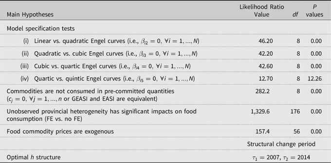
Note: The GEASI specifications are estimated on household food expenditure panel data obtained from the FSSS of Russian Federation. The data cover 67 oblasts/administrative units over the period 2006–2016 and include 7 widely consumed food commodity groups and a numeraire good (i.e., the remaining food and non-food items). A total of 5,896 observations have been utilized in the demand system estimation.

To shed light on the effects of the restrictive assumptions examined above, we evaluate the effect on own-price and income elasticity of demand resulting of the omission of (i) pre-committed demand; (ii) regional fixed-effects, and (iii) supply side of the agricultural commodity price determination mechanism. As can be observed from online supplementary appendix, the own-price and income elasticity differences appear to be statistically and economically significant for a majority of food commodities in our sample. Therefore, future studies should take advantage of these flexible modeling strategies, especially when analyzing various policies concerning such important aspects of economies as food consumption, population health, foreign trade, and food security.

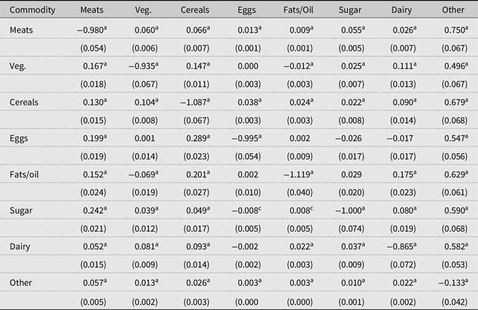
Table 3 presents the demand parameter estimates from the full model. Importantly, pre-committed demand is found to be positive and statistically significant for meats (24.8 kg or 36.7% total meat consumption), cereals (72.1 kg or 60.4% total cereal consumption), and vegetable oils (5.3 kg or 42.4% total vegetable oil consumption). These results indicate the lack of Russian consumer flexibility when purchasing these food commodities (in the same vein, consumers appear to be relatively more responsive to income and price changes when purchasing the remaining commodities). Additionally, time variable parameter estimates are insignificant for pre-committed demand across all the equations, which suggests that this demand component has not been subject to structural preference change over our sample period. Table 4 provides the parameter estimates from the reduced-form price equations. It can be seen that many estimates are statistically significant and are compatible with supply side effects on prices. For example, higher temperatures are found to have negative effects on food prices due probably to their favorable effects on crop production.

Table 3. Parameter estimates from the GEASI expenditure share equations

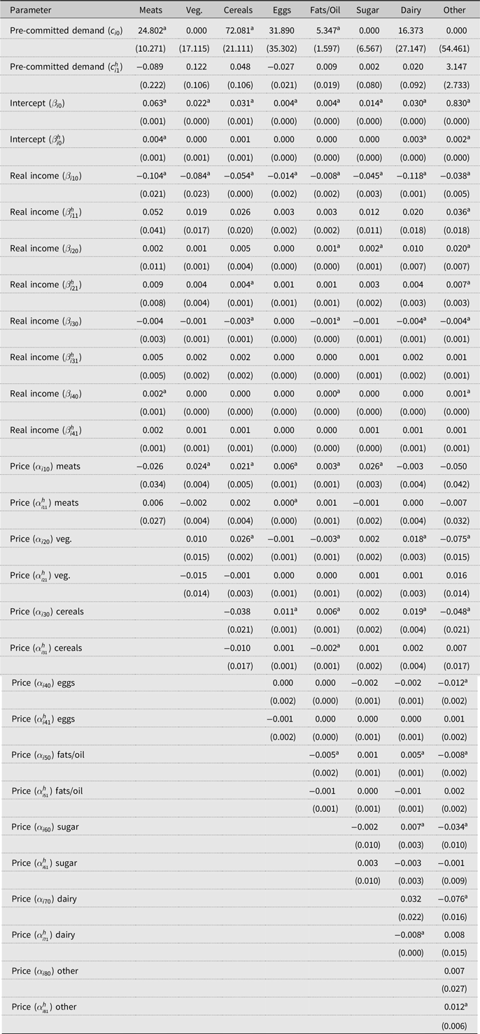
^{a, b, c}Parameter estimates that are statistically different from 0 at the 0.01, 0.05, and 0.10 significance levels, respectively.

Note: The standard errors are in parenthesis.

Table 4. Parameter estimates from the reduced-price equations

^{a, b, c}Parameter estimates that are statistically different from 0 at the 0.01, 0.05, and 0.10 significance levels, respectively.

Note: The standard errors are in parenthesis.

Tables 5 and 6 report the Marshallian, Income and Hicksian elasticity estimates, all of which appear to be consistent with consumer theory. Specifically, Marshallian own-price elasticity estimates are negative, statistically significant, and fall in the range of −1.11 for fats/oil to −0.88 for dairy, pointing to the fact that despite the lack of substitutes for these aggregately defined food commodities, Russian consumers are generally price-sensitive. Our own-price elasticities of demand for cereals (−1.11) and dairy (−0.88) are similar to those provided in other studies (e.g., Burggraf et al., Reference Burggraf, Kuhn, Qi-ran, Teuber and Glauben2015; Hovhannisyan and Shanoyan, Reference Hovhannisyan and Shanoyan2019; Staudigel and Schröck, Reference Staudigel and Schröck2015). However, our own-price elasticity for meats (−1.03) is larger in absolute value vis-à-vis the respective estimates in Goodwin et al. (Reference Goodwin, Holcomb and Shiptsova2002), Staudigel and Schröck (Reference Staudigel and Schröck2015), and Hovhannisyan and Shanoyan (Reference Hovhannisyan and Shanoyan2019), due perhaps to our inclusion of pre-committed consumption and addressing of price endogeneity. Our income elasticity varies from 0.62 for dairy to 1.05 for other food and non-food products and services, which agrees with the Engel’s law and the findings from Zhen et al. (Reference Zhen, Finkelstein, Nonnemaker, Karns and Todd2013). Income elasticity for meats (0.833) is similar to that in Hovhannisyan and Shanoyan (Reference Hovhannisyan and Shanoyan2019). However, our estimate is considerably higher than that in Goodwin et al. (Reference Goodwin, Holcomb and Shiptsova2002).Footnote ¹¹

Table 5. Marshallian price and income elasticity estimates from the GEASI system

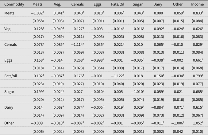
^{a, b, c}Parameter estimates that are statistically different from 0 at the 0.01, 0.05, and 0.10 significance levels, respectively.

Notes: The standard errors are in parenthesis. The first column represents commodities with price change.

Table 6. Hicksian elasticity estimates from the GEASI system

^{a, b, c}Parameter estimates that are statistically different from 0 at the 0.01, 0.05, and 0.10 significance levels, respectively.

Notes: The standard errors are in parenthesis. The first column represents commodities with price change.

To examine the effects of structural food preference change on the elasticity estimates, we use paired t-test of difference to compute the change in Marshallian price elasticity estimates over the span of 2006–2015 (Table 7). Our findings indicate that all Marshallian price effects have undergone significant changes, with a majority of own-price estimates having increased in magnitude (i.e., became more negative). We further compute provincial-level income and price elasticities to illustrate the effects of structural preference change across commodities and provinces. The income elasticity estimates graphically presented for select commodities such as vegetables (Figure 1, Panel A) and meats (Figure 1, Panel B) may be indicative of vegetables having gained popularity as is evidenced by the rising magnitude of the respective income elasticities of demand, while consumer preferences for meat products (and cereals, as can be seen in Figure 2) have declined in the majority of the provinces in our sample, suggesting perhaps consumer saturation in these food categories.

Table 7. Change in Marshallian price elasticity estimates induced by preference change

^{a, b, c}Parameter estimates that are statistically different from 0 at the 0.01, 0.05, and 0.10 significance levels, respectively.

Notes: The standard errors are in parenthesis. The first column represents commodities with price change.

Note: Elasticities for 2006 appear in blue, and those for 2015 are in red.

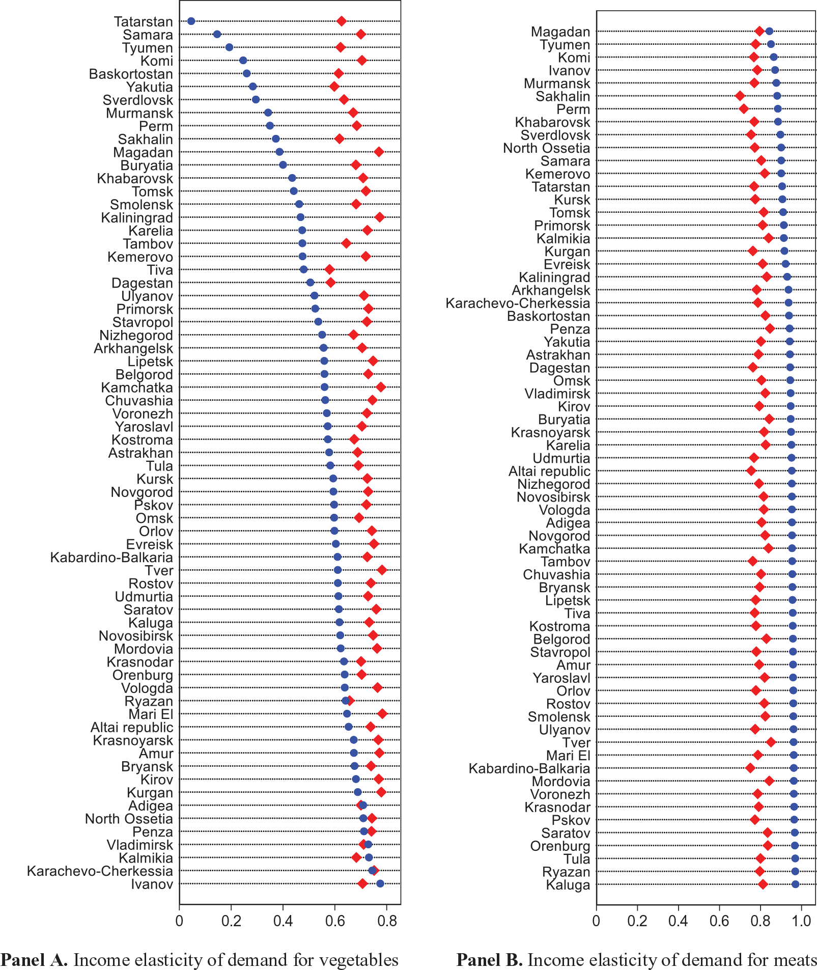
Figure 1. Provincial-level income elasticity of demand for vegetables and meats in 2006 and 2015.

Note: Elasticities for 2006 appear in blue, and those for 2015 are in red.

Figure 2. Provincial-level income elasticity of demand for cereal products in 2006 and 2015.

As a final exercise, we evaluate consumer welfare effects of actual food price changes in Russia over our sample period, with allowance made for structural food preference changes. This analysis is important, given that the rapid rise in food prices brought by global commodity price spikes over 2006–2008 adversely affected a number of countries and created serious welfare concerns among the population segments most vulnerable to food price volatility (Attanasio et al., Reference Attanasio, Di Maro, Lechene and Phillips2013). We perform this computation for all the provinces under study based on the compensating variation (CV) method that utilizes compensated elasticity estimates obtained from our empirical framework, as well as the actual food price changes for the seven food aggregates. Online supplementary appendix reveals that the per capita average annual CV estimates range from 2,500 Rubles (about $83) for Tambov to 7,000 Rubles (about $233) for Magadan, indicating a welfare loss that an average Russian consumer has undergone annually over 2006–2016. When extrapolated to the entire sample period of 11 years, these estimates are equivalent to $913 for Tambov and $2,563 for Magadan, computed on a per capita basis. We further evaluate the difference in the estimates of the welfare consequences of actual price changes in the country, as well as those of hypothetical scenarios of 15% and 25% uniform price increases, resulting from ignoring food preference changes. The respective CV estimates are found to be positive under both frameworks that ignore and address structural food preference transition, which is indicative of welfare loss. We find that disregarding preference dynamics overstates the welfare loss by $37 million for the actual price changes, and by $46 million and $77 million for the simulated uniform price increase by 15% and 25%, respectively.Footnote ¹² These estimates further illustrate the importance of understanding potential food preference changes in Russia.