


Introduction
Depending on its thermal history, growth conditions and age, sea ice contains typically 5–50% of the salts dissolved in the sea water from which it grows. While the composition of sea salts is rather constant in the world ocean, considerable variation of the proportions of ions has been observed in sea ice (e.g. Reference TsurikovTsurikov, 1974; Reference Weeks, Ackley and UntersteinerWeeks and Ackley, 1986). Note that in standard sea water the six major ions account for ∼99.35% of the overall mass of dissolved salts: 55.03% Cl − ; 30.66% Na+; 3.65% Mg2+; 7.71% SO4 2− ; 1.17% Ca2+; and 1.13% K+. For a recent review, see Reference Millero, Feistel, Wright and McDougallMillero and others (2008). This observation has often been associated with the temperature-dependent formation of cryohydrates from concentrated sea-water brine, first illustrated by Reference Pettersson, ld, Stockholm and BeijersPettersson (1883). This has since been studied in detail by chemical analysis of laboratory-grown ice (Reference Anderson and JonesRinger, 1906; Reference GittermanGitterman, 1937; Reference Nelson and ThompsonNelson and Thompson, 1954). These early studies agreed on the following findings for the major sea-water ions during freezing:
-
1. Sulphate and sodium precipitate near –7 to –8 ˚ C in the form of mirabilite (Na2SO410H2O).
-
2. Hydrohalite (NaCl6H2the dominating sea salt, pre-O), cipitates close to –22.9 ˚ C.
-
3. the last two major ions, Mg2+ and K+, do not precipitate above ∼–34 ˚ C.
On the basis of these results, Reference AssurAssur (1960) inferred a composition phase relationship of sea ice which was later refined by Reference RichardsonRichardson (1976). Both authors proposed the crystallization of MgCl28H2O at ∼–18 ˚ C. More recently, Reference Marion, Farren and KomrowskiMarion and others (1999) confirmed by thermodynamic simulations much of the phase relationship, with some exceptions. Their model did not reveal the ∼–18 ˚ C transition for the octahydrate of magnesium and chlorine, and simulated a eutectic temperature for mirabilite precipitation of –6.3 ˚ C (slightly higher than proposed on the basis of laboratory studies). They also noted that, depending on freezing conditions, different pathways might exist below ∼–22 ˚ C where the redissolution of mirabilite, a precipitation of gypsum (Ca2SO42H2O), could occur.
While some details of the sea-water phase diagram have yet to be clarified, the principal result has remained. Major sea-water compositional changes will occur when mirabilite and hydrohalite precipitate as cryohydrates near −7 and −23 ˚ C, respectively. Ion fractionation in bulk sea ice will then depend on whether brine and salt crystals become separated and remain in the ice. For example, the enrichment of SO4 2 − with respect to Cl − (e.g. Reference TsurikovTsurikov, 1974; Reference ReeburghReeburgh and Springer-Young, 1983) indicates that mirabilite, once crystallized, remains in the ice that continues to exchange its brine against sea water. on the other hand, the depletion of sulphate would not only require that the mirabilite crystals leave the ice, but also that they leave some residual depleted brine behind. Observations of old, low-salinity ice samples (Reference ReeburghReeburgh and Springer-Young, 1983; Reference MeeseMeese, 1989) indicate that sulphate is depleted during ageing. However, sulphate depletion has also been found locally in bands of young sea ice (Reference Bennington and KingeryBennington, 1963; Reference AddisonAddison, 1977) and for entire young ice cores in the field (Reference Anderson and JonesAnderson and Jones, 1985). It is currently unclear what conditions determine sulphate depletion and if it is an exception during the growth season.
A more puzzling aspect was reported by Reference Lewis and ThompsonLewis and Thompson (1950) in an early laboratory study of the temperature dependence of sulphate fractionation during freezing. They found maximum SO4 2− /Cl − enrichment for ice that had not cooled below –8 ˚ C. Analysing data from different Russian investigators, Reference TsurikovTsurikov (1974) also emphasized that high probabilities of enrichment in Mg2+ and depletion in K+ were difficult to explain with the proposed phase relation from Assur (1960); temperatures below –30 ˚ C were unlikely for the natural sea-ice samples in question. Similar conclusions may be drawn from further laboratory experiments (Reference AddisonAddison, 1977; Reference Granskog, Virkkunen, Thomas, Ehn, Kola and MartmaGranskog and others, 2004) and field studies in the Baltic Sea (Reference Granskog, Virkkunen, Thomas, Ehn, Kola and MartmaGranskog and others, 2004) and Arctic Ocean (Reference MeeseMeese, 1989). the observed Mg2+ enrichment and K+ depletion cannot be explained by cryohydrate formation on the basis of the presently established eutectic temperatures. Some authors have therefore suggested a revision of the sea-water phase diagram (Reference TsurikovTsurikov, 1974; Reference MeeseMeese, 1989), while others have suggested the possible role of selective ion adsorption or diffusion (Reference Lewis and ThompsonLewis and Thompson, 1950; Reference Malo, Baker and GouldMalo and Baker, 1968; Reference Granskog, Virkkunen, Thomas, Ehn, Kola and MartmaGranskog and others, 2004).
In the present paper, we address these questions of ion fractionation through a study of very young (2–3 weeks) Arctic sea ice, of which few systematic observations exist. To investigate the mechanism of fractionation, we determined the concentration of ions in bulk ice, centrifuged brine and residual ice. We first describe our techniques and sampling approach and give an overview of the general conditions under which the sea ice formed and transformed. After presentation of the results, we interpret them with respect to previous work.
Sampling and Data Analysis
Sea-ice sampling and sample processing
Sea-ice sampling was performed during March 2009 in Kongsfjorden, Svalbard (Fig. 1; Table 1). Repeated sampling (stations 1, 2 and 4) was performed during four successive days ∼500m from the harbour of Ny Ålesund, accessible within a walk of 15 min from the Arctic Marine Laboratory where part of the analysis was performed. Station 3 was obtained 200 m offshore from the harbour within somewhat thicker ice. Two further sampling sites (5 and 6) were located 10 km to the east and accessed by snowmobiles.

Fig. 1. Field sampling in Kongsfjorden, Svalbard, during March 2009: (a) sampling locations and (b) meteorological conditions in Ny Ålesund during (approximate) freeze-up and sampling 2–3 weeks later. Dates are day/month.
Table 1. Sea-ice sampling conditions; superscript numbers indicate the observed variation in the last digit(s). Except for S Water, these variations are larger than the measurement errors. Stations 1, 2 and 4 (denoted with r ) were located at the same site

Ice cores were obtained with a 7.25 cm diameter coring device (Mark III, Kovacs Enterprises), immediately cut into 3–4 cm thick subsamples and packed in their natural orientation into conical lockable plastic beakers. By this method we also collected the brine at the bottom of the beakers that drained prior to centrifugation (in most cases a small fraction and generally <10% of the total drained plus centrifuged brine).
On a first ice core, temperatures were measured with a penetration probe. These bulk ice samples were later melted for electrolytic conductivity and ion concentration measurements. For a second core, different procedures were applied at different stations. At stations close to Ny Ålesund, the plastic boxes were packed into Styrofoamor small dewars and rapidly (within 20 min) transported to the laboratory, where they were set into temperature-controlled freezers (WAECO Coolfreeze T56). the freezers had been preset close to the sample in situ temperatures estimated from an initial surface temperature measurement. the largely linear temperature profiles of the thin ice, with lowest temperatures at the surface, allowed this simple procedure. Due to the small temperature range of the ice cores (1–1.5 K for the thinnest and 3–4 K for the thicker ice) the preset values in most cases agreed with the actual observations within 0.3– 0.5 K. For the remote stations, the temperature-controlled boxes were transported by snowmobiles to the field sites and either powered by the engines or an aggregate. Samples were then directly placed into the corresponding temperature boxes. the procedure ensured that samples to be centrifuged in the laboratory remained close to their respective in situ temperatures. At every station, at least one core for bulk ice and centrifuging was obtained.
After a maximum of 1–2 days of storage in the laboratory, the samples were centrifuged at their respective temperatures. After cooling the centrifuge (Sarstedt LC 1K with minimum –30 ˚ C) for 30 min, specially prepared plastic beakers were set into the stainless-steel beakers of the rotor and centrifuged for 15 min. Since many of our samples were very warm and relatively soft, a value of 10g (10 × gravitational acceleration) was selected. For 3–4 cm thick samples, this corresponds to a pressure of ∼3–4 kPa, well below the lowest tensile strength values (20–50 kPa) observed for natural sea ice (Reference Weeks, Ackley and UntersteinerWeeks and Ackley, 1986). the centrifuged brine was collected and added to the (generally small) amount of brine that had drained during storage in the sample beaker. Its mass was measured and, after equilibration to room temperature, its electrolytic conductivity. the centrifuged ice was immediately packed into plastic bags and put into a –80 ˚ C freezer.
In a further cutting procedure, the ice samples were reduced to 2×2 cm sized cylinders in order to fit them into sample holders for synchrotron-based X-ray microtomography (SXRT) imaging. To minimize the metamorphosis of the centrifuged samples, they were kept near –80 ˚ C prior to imaging by transport and storage on dry ice. During the imaging process, temperatures were kept below –40 ˚ C. SXRT then yielded three-dimensional non-destructive images of 1.3–1.6 cm diameter and 1.7 cm height with 11.84 μm voxel resolution. Compared to earlier methods, SXRT has a large potential to improve the understanding of sea-ice physics (Reference MausMaus and others, 2010). the method exceeds the resolution of recent conventional tomography applications (Reference Golden, Eicken, Heaton, Miner, Pringle and ZhuGolden and others, 2007; Reference Pringle, Miner, Eicken and GoldenPringle and others, 2009) by a factor of four in our case. Analysis of these first SXRT images of natural sea ice is ongoing and will be described elsewhere. For the present study, the images have merely been used to distinguish granular from columnar ice (Fig. 2).

Fig. 2. Horizontal images of 13 cm thick young sea ice, obtained by non-destructive SXRT, at a temperature ≤–40 ˚ C. Air (revealing centrifuged brine) appears bright, ice is grey and residual salt crystals are dark. Left: granular ice ∼2 cm from the surface; right: columnar ice ∼6 cm from the ice–water interface, showing the well-known lammelar plate structure.
Salinity and conductivity
Electrolytic conductivity measurements were performed on melted bulk ice, melted residual ice samples and the centrifuged brine. Conversion to salinity was made using standard equations (e.g. Reference Millero, Feistel, Wright and McDougallMillero and others, 2008). the WTW Cond340i instruments used, with nominal accuracy of 0.5% for conductivity, were first calibrated with a standard KCl solution and later checked for consistency with a conductivity–temperature–depth (CTD) instrument (SD 204, Saiv A/S). the instrument accuracy was 0.03 for salinity and 0.01 K for temperature (this instrument was also used for profiling the water column below the ice to 30 m depth). Ice and brine salinities obtained in this way have an accuracy of better than 0.2. the CTD-derived sea-water salinities, also used for validating the chemistry measurements, have a relative accuracy of 0.1%.
Chemistry
The melted ice and brine samples were kept dark and at a temperature of 4
˚
C before being analysed in the Laboratory of Radiochemistry and Environmental Chemistry of the Paul Scherrer Institute, Villigen, Switzerland. Concentrations of the six major sea-water ions (Cl
−
, Na+, ![]() , Mg2+, Ca2+ and K+) were obtained by standard ion chromatography (IC). Instead of comparing absolute concentrations we investigate the relative deviation of the ratio of these ions to chlorine CX /C
Cl
− from that of Standard Mean Ocean Water (SMOW), i.e.
, Mg2+, Ca2+ and K+) were obtained by standard ion chromatography (IC). Instead of comparing absolute concentrations we investigate the relative deviation of the ratio of these ions to chlorine CX /C
Cl
− from that of Standard Mean Ocean Water (SMOW), i.e.
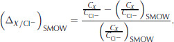
This fractionation measure, first applied by Reference TsurikovTsurikov (1974) to sea ice, makes different salinities and thus the results for ice and brine samples comparable. It also has the advantage of cancelling dilution errors. SMOW ratios are taken from Reference Millero, Feistel, Wright and McDougallMillero and others (2008, Table 2).
From observations by other authors (e.g. Reference Pettersson, ld, Stockholm and BeijersPettersson, 1883; Reference WieseWiese, 1930; Reference Anderson and JonesAnderson and Jones, 1985) we expect that the sea-water ΔX/ Cl − signatures are stable during winter and deviate by <1% from SMOW. To validate our procedure we compare seven sea-water samples resembling winter conditions in Svalbard waters. Four samples were obtained during our fieldwork from 5–20m depth below the ice, while three samples were acquired from Storfjorden.
Figure 3a depicts the relative deviations of absolute concentrations of any ion (including chlorine) from SMOW, and Figure 3b depicts the fractionation (ΔX/ Cl −)SMOW. Prior to IC analysis we often diluted Ca2+ and K+, present in normal sea water as ∼2% weight fraction of Cl − , to concentrations less than 20 times the detection limit (shown in Fig. 3 as thin vertical bars). This dilution may explain the large scatter and a standard deviation of 5–7% for these ions. For SO4 2− and Mg2+ we found a significant systematic deviation of ΔX/ Cl − from SMOW, which we attribute to an uncertainty of ∼5% in the IC calibration and analysis. We therefore reference all results in the following to our slightly different sea-water measurements in Figure 3b.

Fig. 3. Ionic composition of winter sea-water samples from Svalbard: (a) relative deviations from SMOW concentrations for each ion and (b) fractionation or relative deviation of ionic ratios X ion / Cl − from SMOW. the average of seven samples, each processed twice, is shown with ±1 standard deviation (large symbols and thick bars), observations as dots and detection limits as thin bars. the salinity is scaled such that the ticks marking S = 35 for each ion are spaced by 5 units. Two samples with highest salinities are from a laboratory experiment.
Results
Sea-ice growth conditions
The meteorological conditions during and prior to sampling are summarized in Figure 1b. We used daily ice charts produced by the Norwegian Meteorological Institute (mainly based on observations from different satellites), information on freeze-up by the local station staff, our classification of granular/columnar ice as well as other information in Table 1 to propose the following ice-growth history.
Kongsfjorden was ice-free during the exceptionally warm January of 2009. After 2 weeks of persistent low temperatures, some fast ice originated in the inner fjord by mid-February. A warming event with 4 cm of precipitation (17–21 February) was then followed by strong winds and moderate cooling (–14 to –15 ˚ C). This likely created a slushy snow ice cover in many places which then froze under calm cold conditions (–15 to –19 ˚ C) during 25–28 February. on 1 March, temperatures rose again to –14 ˚ C and the first 2mmw.e of snow were deposited on the ice; temperature subsequently rose again (to –10 to –4 ˚ C). Another centimetre of precipitation fell during the following week. the daily average temperature then rose over 2 days to a maximum of –2.4 ˚ C on 9 March. on the first two days of our sampling programme (10 and 11 March), temperature had decreased to –4 to –5 ˚ C. the temperature then fell again and remained mostly between –19 and –15 ˚ C during the other sampling days.
The largest thickness of granular ice from all cores found from the surface downwards was 23 cm (almost the entire core) at station 3 closest to the harbour. This was similar in a bay east of the harbour, likely reflecting the wind-enhanced onshore accumulation of snow slush 2 weeks prior to sampling. the ice at stations 5 and 6 in the inner fjord (Fig. 1a) was thicker. In the structural core of the easternmost station 5, the upper 12 cm of the 32 cm was granular with large grains, followed by an 8 cm transition layer with both columnar and granular ice. At the slightly more western station 6, both the granular ice thickness of 6–7 cm and the total thickness of 22 cm were lower. From the mentioned 4 cm of precipitation between 17 and 21 February, we would expect (assuming a solid packing fraction of 0.4–0.5) an average snow-ice thickness of ∼7–9 cm. Higher thicknesses may accumulate near barriers and coasts. In this sense, the largest eastern granular ice thickness was consistent with the proximity of this station to a shallow called Breskjera. Taking this aspect into account, we suggest that despite varying in thickness the ice at stations 3, 5 and 6 formed at the same time (i.e. 2–3 weeks prior to sampling).
The repeated site (stations 1, 2 and 4) was 300m further offshore than station 3. It only showed 3–4 cm of granular ice at the surface of thinner (13–14 cm) ice. Near this site, which was close to the bottom slope towards the 200m deeper central Kongsfjorden, we observed thin ice and permanent leads. the near-surface water temperatures of –1.5 ˚ C (0.4K above the freezing point) and higher values of –0.9 to –1.0 ˚ C at 20m depth highlight the role of upwelling Atlantic Water in retarding ice growth.
Hydrographic conditions measured by CTD at stations 1–4, which indicate a weakly stratified water column with salinities of 34.3 and 34.4 near the surface and at 20m depth, respectively, favour such upwelling of heat. In contrast, the 20m temperatures were much lower (–1.5 to –1.7 ˚ C) at the eastern stations. Lower near-surface temperatures also indicate that such effects are limited. Considering the precipitation record also, we suggest that this ice has very likely formed 2–3 weeks prior to sampling but has grown less rapidly.
Brine, bulk and residual ice salinity
Profiles of bulk ice salinities for the repeated station (1, 2 and 4) of primarily columnar ice are shown in Figure 4a. an interesting aspect to be discussed is that the ice salinity increased in a stage of warming and slight melting from 10 to 11 March, and then decreased again.
In addition to the bulk salinity, centrifuging provides (1) the hydrodynamically accessible salt fraction and (2) the salt fraction that is hardly extractable, located in disconnected voids or dead ends. the residual salt fraction that remained in the ice after centrifugation as a function of the total volume fraction of brine in the bulk ice is shown for all samples in Figure 4b.

Fig. 4. (a) Bulk ice salinity profiles for the ∼14 cm thick ice during the course of three days at the repeated site (stations 1, 2 and 4) and (b) residual salt fraction (for all stations 1–6) after centrifugation as a function of the overall brine volume fraction in the bulk ice.
For measured salinity and mass of brine (S b and m b) and residual centrifuged ice (S r and m r), the bulk ice salinity is given as
We define the residual salt fraction f r (non-dimensional) as the ratio of non-centrifugable to total mass of salt in the bulk ice:
Under thermodynamic equilibrium, f r is equivalent to the ratio of residual to total brine volume.
The residual salt fraction f r was computed assuming thermodynamic equilibrium with the freezer temperatures, using equations for brine volume from Reference Cox and WeeksCox and Weeks (1983). Our ensemble mean of 0.35 ± 0.09 for the salt fraction that remained in the ice is slightly larger than 0.2– 0.3 obtained by Reference Weissenberger, Dieckmann, Gradinger and SpindlerWeissenberger and others (1992) for older ice in the Southern Ocean, yet comparable to laboratory data of young ice summarized in Reference MausMaus and others (2010). We do not yet know if this difference may be attributed to different ice age and structure or is due to our order-of-magnitude smaller centrifuge acceleration, resulting in the incomplete removal of interconnected brine. the loss of brine would also overestimate the entrapped salt fraction. Since the samples were rapidly placed in beakers to collect brine draining prior to centrifugation, this effect was likely small.
Ion fractionation: brine versus residual ice
We now describe the fractionation of the major sea-water ions with respect to chlorine. Brine, bulk ice and residual ice salinities and ion concentrations scale in our observations typically as S b : S i : S r ∼15 : 3 : 1. We compare them in Figure 5 on a logarithmic scale of the observed Cl − concentration. Brine samples appear as triangles at the high end, residual ice samples as circles at the low end and bulk ice samples as squares in between. For every observation a bar shows either the detection limit or standard error from the sea-water sample calibration in Figure 3, whichever is larger. We also show snow samples and indicate upper ice (3–4 cm) samples exposed to the lowest temperature.

Fig. 5. Ion fractionation for all samples from stations 1–6, comparing brine, bulk ice and residual ice after centrifugation. the vertical bars are the detection limits or one standard error from the sea-water calibration, whichever is larger. Note the different scales for the ions. Surface ice samples are indicated as black dots, and snow samples are shown as stars. A cross on the abscissa indicates the Cl − concentration 19 353 ppm of standard sea water (SMOW) with salinity 35.
Statistics of these groups are summarized in Table 2. In addition, we compute statistics of the difference between brine and residual ice for the two warmest ice cores 1 and 2 (see Table 1).
Table 2. Ion fractionation in young sea ice from Kongsfjorden. Values in parentheses after the class averages are the p-level of the Student’s t test; numbers in italics indicate the 95% level. Superscript a denotes that the t test is passed at 95% but the signal is not larger than the standard error of the sea-water reference measurements from Figure 3b

For sodium ions (Fig. 5a) no dependence on sample type (residual ice, brine, bulk ice, snow) or chlorine concentration was evident. Most observations lie in the range –0.04 to +0.04. We found 0.5–1% fractionation in most samples, differing from 0 at significance levels of 90–95%, with the higher values and significance for the surface and brine samples (Table 2). However, all signals are similar to the uncertainty of our sea-water standard calibration. A few exceptionally low values indicate the method’s reproducability and also appear in Figure 5b and c for the fractionation of Mg2+ and Ca2+. For magnesium ions (Fig. 5b) the spread is somewhat larger, but a significant difference between the ice types (or surface samples) is not present.
The distribution of sulphate ion fractionation (Fig. 5c; third column in Table 2) indicates two findings. First, almost all surface and snow samples (indicated as black dots) show positive values and thus enrichment in sulphate. Second, the brine samples show a clustering of particularly low fractionation values (depletion) at lowest chlorine concentrations in the range 15 000–20 000 ppm Cl − . These samples are from the warmest stations 1 and 2 where centrifuged brine salinities were low. Depletion is found to be highly significant in the difference of brine and residual ice at these two stations (p = 0.004 in Table 2).
The calcium ion does not show a significant fractionation in any of the groups (Fig. 5d). Most observations fall between –0.1 and +0.1, a spread comparable to the standard error.
The most noteworthy ion is potassium. In all classes except the bulk ice (with the smallest number of 20 samples) the hypothesis of zero fractionation is rejected at high levels of significance (fifth column in Table 2). In contrast to SO4 2− , the most anomalous behaviour is observed in the residual ice which is considerably depleted in potassium (Fig. 5e). A low-salinity snow sample behaves in the same manner. To emphasize this signature, in addition to ΔK+/ Cl − the potassium fractionation with respect to Mg2+ is also shown in Figure 5f, revealing similar results.
Depth and time dependence
The significant fractionation results for ![]() and K+ were investigated further by focusing on their depth dependence. the repeated site observations have been averaged at four depths of the 14 cm thick young ice. the mentioned surface enrichment of sulphate in Figure 5c is seen in the ice profile in Figure 6a. Sulphate depletion is seen at all depths below the surface in brine and residual and bulk ice, but is most pronounced in the brine. Figure 6b shows that the depletion of K+ in the residual ice was found at all depths. Figure 6a, c and d indicate for
and K+ were investigated further by focusing on their depth dependence. the repeated site observations have been averaged at four depths of the 14 cm thick young ice. the mentioned surface enrichment of sulphate in Figure 5c is seen in the ice profile in Figure 6a. Sulphate depletion is seen at all depths below the surface in brine and residual and bulk ice, but is most pronounced in the brine. Figure 6b shows that the depletion of K+ in the residual ice was found at all depths. Figure 6a, c and d indicate for ![]() , Na+ and Mg2+ an upwards increase of enrichment with respect to chlorine. the same behaviour is found for the snow on top.
, Na+ and Mg2+ an upwards increase of enrichment with respect to chlorine. the same behaviour is found for the snow on top.

Fig. 6. Ion fractionation averaged for different depths for the repeated station (1, 2 and 4). the upper values are snow samples, while the sea-water zero fractionation reference is emphasized as a dashed vertical line with its uncertainty as a horizontal bar. Slightly larger error bars for the ice and snow values (see Fig. 7) have been omitted for clarity.
As bulk ice samples consist of brine and residual ice, their signatures should fall between them. This is only the case for K+ (Fig. 6b) and consistent with high significance for this ion alone. As shown in Table 2, the results are generally less significant for the relatively small (n = 20) set of bulk ice samples. As these stem from close but different ice cores, the difference may be natural variability. To investigate this question further, we focused on the time dependence of the non-surface (3.5–14 cm) part of the repeated station over the course of three days. In Figure 7a it is seen that while the SO4 2− fractionation in the residual ice did not change during this period, the brine signal changed from depletion to the neutral residual ice level. the bulk ice signature follows the residual ice signature. the brine fractionation also approaches the residual ice level that remains depleted for K+ (Fig. 7b). Here, however, the bulk ice signature shift is similar to the brine. Figure 7 indicates that signatures in brine and bulk ice are much more variable than in the residual ice.

Fig. 7. Temporal evolution of fractionation of (a) ![]() , (b) K+ and (c) Na+ averaged over the 3.5–14 cm columnar ice from the repeated stations 1, 2 and 4. Dates are day/month in 2009. For clarity, values for brine, residual ice and bulk ice are shown slightly lagged.
, (b) K+ and (c) Na+ averaged over the 3.5–14 cm columnar ice from the repeated stations 1, 2 and 4. Dates are day/month in 2009. For clarity, values for brine, residual ice and bulk ice are shown slightly lagged.
Discussion
The goal of the present work was to study the details of chemical fractionation during the formation of sea ice in order to better understand earlier findings of its variability. By sampling, transport and centrifugation of sea ice at its in situ temperature, we have separated samples into (1) the hydrodynamically accessible salt fraction and (2) the part of brine that cannot be extracted, being either disconnected in brine pockets or located in dead-end pores. the analysis was performed on 3–4 cm subsampled profiles of young ice aged 2–3 weeks. In addition to the spatial resolution, one site was repeated while the ice changed from a warm stage of internal melting to a more solid refrozen stage. For most stations we also determined the fractionation of bulk ice cores.
In our data analysis we found three robust results: (1) SO4 2− was found to be depleted in brine samples (5%), particularly during the days when the ice was warmest (stations 1 and 2); (2) K+ showed strong depletion (5–15%) in all samples, with maximum values in the residual ice significantly larger than in the brine; and (3) SO4 2− (and to some degree Na+) is enriched in surface ice and snow.
Considering the mentioned eutectic temperatures and the thermal history of the analysed young ice (Fig. 1), we expect the formation of mirabilite (Na2SO410H2O) as the only precipitation signal for these ions. the eutectic temperatures where Cl − , K+ and Mg2+ are believed to precipitate have not been reached. Also, using the meteorological conditions in one-dimensional heat flux estimates to match the moderate growth rates (not shown), we find it unlikely that the thin ice near the harbour has been cooled to temperatures less than −8 ˚ C. Assuming a linear temperature gradient in the ice and a temperature of −6.3 ˚ C for mirabilite precipitation (Reference Marion, Farren and KomrowskiMarion and others, 1999), we only expect it in the surface samples of stations 1–4. This is qualitatively consistent with the profiles in Figure 6a, showing higher SO4 2− concentration near the surface. We further estimated that, for the thicker ice at stations 5 and 6, the critical temperature may have been reached in the upper third of the ice. the significant surface enrichment of sulphate (Fig. 5c; Table 2) derives strongly from stations 5 and 6 (not shown). the question remains, however, what may explain the depletion of SO4 2− in the brine at stations 1 and 2 and of K+ in most residual ice?
We first considered the possibility that, even if average daily temperatures did not cool the ice below –6.3
˚
C, daily temperature extrema may have done so and also led to mirabilite precipitation below the surface. We note that the depletion of SO4
2−
in the brine was limited to the warm stations 1 and 2, and disappeared when the ice at stations 1 and 2 cooled and likely refroze internally (Fig. 7). We therefore suggest that during warming the pores may have widened without dissolution of the (presumably present) mirabilite crystals. These may then have fallen off the ice, leaving behind depleted brine. While this is plausible, we cannot exclude the possibility that our centrifugation protocol has artificially created this signature (i.e. that mirabilite crystals were centrifuged off the ice yet remained undetected in the collecting beaker). In any case, mirabilite must have formed yet not re-dissolved upon warming, implying its presence at levels where it is not expected on the basis of average growth conditions. As a second explanation we may consider that, when mirabilite is formed near the surface, some remaining brine depleted in SO4
2−
was expelled downwards and decreased the sulphate concentration in the rest of the ice. If SO4
2−
is redistributed in this way, its total vertically integrated concentration in the bulk ice would remain unchanged. This condition would require a ∼0.02 lower true level of zero sulphate fractionation in Figure 6a, still being within one standard error of the sea-water calibration. Both explanations involve the formation of mirabilite, the vertical redistribution of brine and possible loss of both components to sea water, and they cannot be evaluated using the present dataset. (We note that for mirabilite precipitation, creating one unit depletion in ![]() would only create ∼13% depletion in Na+. Our observations are not sufficiently accurate to determine such a signal quantitatively, but support significant surface enrichment of Na+ (see Table 2).) However, the presence of vertical pattern and different fractionation in residual ice and brine, as found for the non-precipitating K+ ion, suggests the possibility of a third mechanism.
would only create ∼13% depletion in Na+. Our observations are not sufficiently accurate to determine such a signal quantitatively, but support significant surface enrichment of Na+ (see Table 2).) However, the presence of vertical pattern and different fractionation in residual ice and brine, as found for the non-precipitating K+ ion, suggests the possibility of a third mechanism.
Depletion of K+, the signal of highest significance that we observe, has to some degree been reported in many earlier studies (Reference TsurikovTsurikov, 1974; Reference AddisonAddison, 1977; Reference MeeseMeese, 1989; Reference Granskog, Virkkunen, Thomas, Ehn, Kola and MartmaGranskog and others, 2004). However, we can exclude the possibility of temperatures where we would expect K+ to precipitate. In particular, the enrichment of K+ in the residual ice with respect to brine points to its origin by a different mechanism: differential molecular diffusion of ions.
To illustrate this we consider a simple model of vertical brine channels connected to fine lateral pore networks in which fluid flow is weak. In our observations, the former corresponds to the centrifuged brine and the latter to the residual ice. We further suggest that the stagnant brine in the residual ice is in thermal equilibrium, and therefore has a higher local concentration than the brine in those channels that take part in intermittent convective exchange with sea water. This sets up (lateral) concentration gradients and creates diffusive solute transport that depends on the molecular diffusivities of the ions. We then expect that those ions that diffuse slower than Cl
−
, namely ![]() Ca+ and Mg2+, will become enriched in the residual ice while the more rapid ion K+ will become depleted.
Ca+ and Mg2+, will become enriched in the residual ice while the more rapid ion K+ will become depleted.
In Figure 8a we show the fractionation contrast between residual ice and brine as a function of the molecular diffusivity of the major ions, estimated by Reference Li and GregoryLi and Gregory (1974) on the basis of electro-neutrality. the enrichment– depletion distribution reasonably scales with ion diffusivity in the expected manner, with maximum depletion of K+ contrasting with maximum enrichment of ![]() While we cannot exclude the possibility that the
While we cannot exclude the possibility that the ![]() depletion derives from brine redistribution during mirabilite formation, this scaling of fractionation with diffusivity is remarkable. We provide further support from a study of Baltic Sea ice by Reference Granskog, Virkkunen, Thomas, Ehn, Kola and MartmaGranskog and others (2004), showing their results in Figure 8b. Disregarding Ca2+, which is likely precipitating at rather high temperatures, enrichment (depletion) also appears to be related to the condition if a specific ion diffuses slower (faster) than chlorine. the robust signatures in Baltic Sea ice are not unexpected as, due to its low porosity and permeability, convective activity is limited, which renders molecular diffusion important.
depletion derives from brine redistribution during mirabilite formation, this scaling of fractionation with diffusivity is remarkable. We provide further support from a study of Baltic Sea ice by Reference Granskog, Virkkunen, Thomas, Ehn, Kola and MartmaGranskog and others (2004), showing their results in Figure 8b. Disregarding Ca2+, which is likely precipitating at rather high temperatures, enrichment (depletion) also appears to be related to the condition if a specific ion diffuses slower (faster) than chlorine. the robust signatures in Baltic Sea ice are not unexpected as, due to its low porosity and permeability, convective activity is limited, which renders molecular diffusion important.

Fig. 8. Fractionation (with respect to Cl
−
) versus molecular diffusivity of several ions; standard deviations shown as vertical bars. Diffusivities are from Li and Gregory (1974) for electro-neutrality at 23.7
˚
C. (a) Difference of residual ice and brine fractionation for the columnar ice (3.5–14 cm) from the multiple sampled young ice at stations 1, 2 and 4. (b) Fractionation of young brackish water ice from the Baltic Sea; smaller symbols indicate spring observations (Reference Granskog, Virkkunen, Thomas, Ehn, Kola and MartmaGranskog and others, 2004). diffusion in complex pore networks, a purely molecular diffusion process may also be operative. A vertical concentration gradient (set up by a temperature gradient) will lead to enrichment (depletion) of slower (more rapid) ions than Cl
−
in the upper part of the ice. the fractionation profiles in Figure 6 may support this: in both the columnar ice (the lowermost three depth levels) and the snow, the fractionation of ![]() and Mg2+ increases upwards yet decreases for the more rapid K+ ion. Unknown loss of brine during sampling may only have biased this fractionation if lost and centrifuged brine had different signatures. For example, if the lost brine had a signature close to sea water (which is plausible near the bottom), then fractionation of brine might be overestimated there. Residual ice signatures would be little affected, however.
and Mg2+ increases upwards yet decreases for the more rapid K+ ion. Unknown loss of brine during sampling may only have biased this fractionation if lost and centrifuged brine had different signatures. For example, if the lost brine had a signature close to sea water (which is plausible near the bottom), then fractionation of brine might be overestimated there. Residual ice signatures would be little affected, however.
The temporal variability in Figure 7, with relatively stable residual ice and more variable brine signatures, is also consistent with the concept of diffusion–convection coupling. Furthermore, during re-cooling and internal re-freezing from 11 to 13 March under still warm conditions when no mirabilite may have formed, there was an increase in the ![]() versus a decrease in K+ fractionation in the brine. For both ions this is the expected signal when freezing and desalination by convection are coupled to differential diffusion.
versus a decrease in K+ fractionation in the brine. For both ions this is the expected signal when freezing and desalination by convection are coupled to differential diffusion.
In addition to this coupling of convection and differential
In our study we were restricted to thin ice and signatures forming over the course of days or weeks. During further vertical ice growth and cooling, and when mirabilite precipitation occurs at different levels, a complicated vertical distribution of sulphate fractionation may evolve. the K+ pattern should, however, still reflect the diffusive–convective coupling. As better understanding of this mechanism requires consideration of the ice character, our first approach in the present study was to compare granular and columnar samples. Disregarding the samples from the surface, we did not find a significant difference between the K+ depletion of granular and columnar ice. Unfortunately, in our young ice, the granular texture was always found on top, which makes it difficult to distinguish the effects of microstructure and vertical position.
To make progress, we need to study the pore network connectivity. A natural macroscopic parameter related to the latter is the salt fraction in the residual ice (not removed by centrifugation) depicted in Figure 4b. While our data (similar to earlier results from Reference Weissenberger, Dieckmann, Gradinger and SpindlerWeissenberger and others, 1992) indicated a slight dependence on brine volume, the entrapped fraction was remarkably constant in the range 0.2– 0.5.We did not find a significant difference between granular and columnar ice, yet note that the three largest residual salt fractions of 0.7–0.8 in Figure 4b are from columnar samples. While high residual fractions are of interest in connection with a pore connectivity threshold, the present data do not extend to the frequently mentioned transition porosity of 0.05 (e.g. Reference Weeks, Ackley and UntersteinerWeeks and Ackley, 1986; Reference Golden, Eicken, Heaton, Miner, Pringle and ZhuGolden and others, 2007). A more detailed analysis of the present tomographic dataset in terms of connectivity and percolation aspects is ongoing.
Conclusion
In most earlier studies, ion fractionation in sea ice has been associated with the formation of cryohydrates at certain eutectic temperatures. Here we have investigated young sea ice of known thermal history and discussed its ion fractionation signatures of centrifuged brine and residual ice.
Based on our finding of significant depletion of the K+ ion, we propose differential diffusion rather than eutectic precipitation as a plausible mechanism (likely relevant for the interpretation of several earlier reports). Although we may not exclude precipitation of sulphate in the present study, we propose that ![]() enrichment, observed earlier in the absence of mirabilite precipitation (Reference Lewis and ThompsonLewis and Thompson, 1950), also appears conclusive in this context since sulphate is the slowest-diffusing major ion in sea water.
enrichment, observed earlier in the absence of mirabilite precipitation (Reference Lewis and ThompsonLewis and Thompson, 1950), also appears conclusive in this context since sulphate is the slowest-diffusing major ion in sea water.
It is remarkable that in both our data and Baltic Sea ice data (Reference Granskog, Virkkunen, Thomas, Ehn, Kola and MartmaGranskog and others, 2004), fractionation scales reasonably with ion diffusivity. Our observations highlight differential diffusion within the sea-ice pore network, rather than in front of the advancing freezing interface (proposed by Reference Malo, Baker and GouldMalo and Baker, 1968), to fractionate ions. We therefore emphasize that the process should be considered when interpreting similar fractionation signals in marine ice cores (e.g. Reference Moore, Reid and KipfstuhlMoore and others, 1994).
Among other topics that we have not touched on here, we mention that calcium carbonate formation and sea-ice surface chemistry (of recent interest due to the impact on gas exchange between the air and sea ice and tropospheric ozone depletion; e.g. Reference DieckmannDieckmann and others, 2008; Reference Marion, Millero and FeistelMarion and others, 2009) may be linked to differential diffusion. the potential to learn about sea-ice physical processes by analysing their chemistry is currently unexplored. the present study highlights the need for good spatial and temporal observations to evaluate the combined effect of convection and diffusion on sea-ice signatures. In particular, the most rapid K+ ion appears to deserve further attention to evaluate models of sea-ice microstructure and phase evolution.
Acknowledgements
We thank the research station staff in Ny Ålesund. We also thank E. Austerheim and A. Kristoffersen from the Arctic Marine Laboratory and E. Borge for his valuable field and laboratory work assistance. We are grateful to A. Eichler and M. Hutterli for support with the IC analysis and E.A. Ersdal for testing the snowmobile-powered temperature boxes. We also thank J.-L. Tison, M. Granskog and two anonymous reviewers for help in improving the manuscript. Tomographic sea-ice images were obtained at the TOMCAT beamline of the Swiss Light Source, Paul Scherrer Institute, Switzerland, with the kind support of the beamline scientists. the project received funding through the project ‘Synchrotron-based X-ray studies of sea ice’, Norwegian Science Foundation and two Arctic fieldwork stipends in 2009 (S. Maus and J. Büttner) from the Svalbard Science Forum.


