


1. Introduction
Shock wave–turbulent boundary layer interaction (SWTBLI) remains among the fundamental problems of modern aerodynamics as adequate modelling has become necessary in the design of efficient control surfaces, high-speed intakes or thermal protection systems. Intensive research, which has been carried out for many years primarily on nominally stationary test configurations, has led to generally good progress in predictability and in understanding phenomena (Dolling Reference Dolling2001; Délery & Dussauge Reference Délery and Dussauge2009; Babinsky & Harvey Reference Babinsky and Harvey2011). However, there are still many open questions, especially concerning unsteady test configurations with forced motions of shock-induced separation.
In reality, the inherently unsteady phenomenon of SWTBLI with mean-flow separation is often superimposed by forced motions of the interacting shock waves, e.g. when operating a rudder or control flap on an aircraft. Although such flows are very relevant in practice, they have hardly been investigated for generic simple-geometry configurations. The reason for this lack of research is the numerous parameters that influence such a flow, such as the Reynolds number, interaction strength, wall thermal condition and travelling velocity of interacting shock waves, making investigations very complicated.
A rough guide value for the mean travelling velocity of the separation shock at a natural large-scale/low-frequency oscillation in the range of ‘quasi-stationary’ SWTBLI was given by Gonsalez & Dolling (Reference Gonsalez and Dolling1993) and independently confirmed in further studies with comparable results (Muck, Bogdonoff & Dussauge Reference Muck, Bogdonoff and Dussauge1985; Dolling & Smith Reference Dolling and Smith1988; Gonsalez & Dolling Reference Gonsalez and Dolling1993; Poggie & Smits Reference Poggie and Smits2000; Beresh, Clemens & Dolling Reference Beresh, Clemens and Dolling2002; Poggie Reference Poggie2019). Notably, the observed trend of decreasing shock oscillation frequency with increasing length of the intermittent region is attributed to the finding that the normalised shock velocity  $U_{trav}/U_{\infty }$ was on average fairly constant at $0.03 \pm 0.01$ and was practically independent of the type of interaction (blunt fin, ramp and sharp fin) and of the size of the intermittent region (Clemens & Narayanaswamy Reference Clemens and Narayanaswamy2014).
With the rough guide value in mind, test configurations can be devised to investigate effects that occur at much higher normalised shock velocities. The independent variation in individual parameters, which must be able to correctly interpret the effects, often fails due to the technical challenges that arise. The most relevant studies carried out thus far in the wide field on the effect of forced, large-scale, shock-front movements are divided into three main groups:
(i) interaction of a steady boundary layer with externally forced oscillating shock fronts (various experimental set-ups based on a cyclic movement or rotation of shock generator by Roberts (Reference Roberts1989), Coon & Chapman (Reference Coon and Chapman1995), Bruce & Babinsky (Reference Bruce and Babinsky2008), Liu & Zhang (Reference Liu and Zhang2011) and Pasquariello et al. (Reference Pasquariello, Hickel, Adams, Hammerl, Wall, Daub, Willems and Gülhan2015));
(ii) interaction between two thin, hot layers extending along the wall or longitudinal coordinate and shocks moving across them (e.g. in the special case of the interaction of an initial shock wave in a shock tube with a thin, hot layer of still air in the area of a locally preheated wall by Hess (Reference Hess1957)); and
(iii) interaction of an unsteady wall boundary layer with a moving normal shock front (specifically, the interaction of a strong reflected shock in the shock tube with the boundary layer on its wall by Mark (Reference Mark1958)).
A detailed review of studies of interacting flows triggered by externally forced oscillating shock fronts (i) is provided in the authors’ earlier publication (Touré & Schülein Reference Touré and Schülein2020). The conclusion presented there is summarised as follows: the realisation of this type of shock excitation in a wind tunnel is quite simple in this way but results in a consistently variable shock intensity and shock-front velocity in the experiment. In contrast, the approaches under points (ii) and (iii) allow a simulation environment with a constant shock-front Mach number, which in principle enables a quasi-stationary consideration of the problem with a coordinate system moving with the shock wave.
Although the assignment of group (ii) seems unexpected, we examine the relevant main results. Hess (Reference Hess1957) was the first to analytically investigate and systematically describe the formation of stagnation bubbles at the foot of a shock wave moving over an encapsulated layer of hot air at rest on a wall. When the shock hits a hot layer, another shock is created that runs into the hot layer, and the interaction starts to build up. To simulate the different possible interaction scenarios, the Mach number of the shock front  $M_{s}$ and the ratio of the temperature of the hot layer to the ambient temperature $T_{hot}/T_{amb}$ were independently varied. The interaction scenario in the coordinate system of the moving shock front was simplified in such a way that a ‘stationary’ solution was sought for each parameter combination. To achieve these steady-state-flow conditions (with respect to the interacting normal shock), the velocities of the shocks travelling inside and outside the hot layer should be equal. This condition only occurs if the pressure and velocity jumps at both shock fronts also coincide.
All stationary interactions were formally divided into subsonic hot-layer interactions and supersonic hot-layer interactions according to the Mach number of the undisturbed hot layer in the shock-bound coordinate system. However, the main subdivision shown in the paper is based on a different feature. The higher the temperature ratio  $T_{hot}/T_{amb}$, the greater are the induced Mach number and the total pressure deficits in the hot core. According to Hess (Reference Hess1957), as soon as the total pressure in the hot layer (or the Pitot pressure in the supersonic case) is no longer high enough to withstand the static pressure increase caused by the main shock, a hot stagnation bubble inevitably forms in the flow, which is enclosed by the ambient air. In the resting reference system, the pressure increase due to the shock is sufficient in this case to entrain the hot layer (accelerate it to the speed of the shock), regardless of whether the hot layer is subsonic or supersonic relative to the shock. Thus, compared with a typical separation bubble in stationary boundary layer flows, this stagnation bubble is mainly characterised by the notion that it is directly bound to the moving shock and can easily occur in a purely supersonic environment.
The flow phenomenon that was described was referred to as the hot spike or thermal spike effect a few years later, when local flow heating in front of blunt supersonic bodies was intensively analysed as a possible measure to reduce their wave drag (e.g. Maurer & Brungs Reference Maurer and Brungs1968; Georgievsky & Levin Reference Georgievsky and Levin1988; Nemchinov et al. Reference Nemchinov, Artem'ev, Bergelson, Khazins, Orlova and Rybakov1994; Knight Reference Knight2008; Schülein & Zheltovodov Reference Schülein and Zheltovodov2011). The validity of the analyses of Hess could be very impressively confirmed and generalised by transferring them to the case of a free, thin, hot layer upstream of a strong bow shock. Again, by localised heating of the air in front of a blunt body, the deficit of the total pressure upstream of the bow shock wave is increased until a free recirculation bubble is created, thus triggering the desired spike effect (Schülein Reference Schülein2016).
Mark (Reference Mark1958) performed one of the first systematic studies of the interaction of a strong reflected shock in a shock tube with the boundary layer at its wall. This situation occurs when the initial shock wave reaches the closed end of the tube, is reflected there and then travels back through the fluid that was set in motion by the initial shock. In the theoretical part of the cited work, simplifying assumptions were made to allow an analysis of this interaction. First, the flow was transferred to the coordinate system moving with reflected shock, in which the shock velocity  $U_{trav}$ in the laboratory system was added to all velocities in the field (figure 1). It was also assumed that the boundary layer can be modelled as a thin inviscid jet, in which the flow has a velocity of the wall ( $= U_{trav}$). Since the wall temperature should correspond to the initial gas temperature in the shock tube, the sound velocity in the initial flow $a_1$ was used to determine the relevant Mach number at the wall $M_{w} = U_{trav}/a_{w} = U_{trav}/a_1$. The local Mach number $M_{w}$ and static pressure $p_{w}$ (behind the initial shock wave) were used to estimate the total pressure $p_{0, w}$ present at the wall. Similar to Hess (Reference Hess1957), Mark (Reference Mark1958) proposed evaluating the existing potential of the boundary layer to overcome the shock-induced pressure rise by comparing the static pressure behind the shock $p_{out}$ with the existing local stagnation pressure $p_{0, w}$. If one transfers these considerations to a stationary SWTBLI ( $U_{trav}=0$), one quickly finds that the formation of a separation bubble would have been predicted at the lowest shock intensity. For this reason, the separation criterion should be estimated as a very low threshold, corresponding to the earliest possible boundary layer separation. Despite this simple approach, Mark was able to map the effects of the separation bubble at the shock-tube wall on the Mach number of the reflected shock in his computational model. Accuracy in predicting the onset of separation at the wall was a minor consideration.

Figure 1. Mach number profile of the boundary layer: (a) wall-bound coordinate system; (b) coordinate system moving with the shock wave.
The underlying concept for a separation criterion based on the Mach number profile of the undisturbed flow is indeed promising. One of the most important features of a supersonic boundary layer is the dependence of the interaction length on, among other things, the thickness of the subsonic layer (e.g. Babinsky & Harvey Reference Babinsky and Harvey2011). With the same path of the Mach number profile in the undisturbed boundary layer, the thickness of the subsonic layer, normalised to the total boundary layer thickness, is approximately inversely proportional to the free-flow Mach number  $M_1$, so that at a high $M_1$, the sonic line remains very close to the wall even at longer run lengths. Since the position of the sonic line is also known to very strongly depend on the locally dominating temperature conditions (Fernholz & Finley Reference Fernholz and Finley1980; Dussauge et al. Reference Dussauge, Fernholz, Smith and Saric1996), the sonic line shifts away from the wall in the case of a heated wall (due to a higher speed of sound) and correspondingly towards the wall in the case of a cooled wall. Thus, as a result of SWTBLI, the distance between the shock impingement point and the induced upstream influence point, which is commonly referred to as the interaction length, can vary greatly depending on the relationship between the wall temperature $T_{w}$ and the recovery temperature $T_{r}$. Various aspects of the wall temperature effect in SWTBLI have already been demonstrated and studied both experimentally (Spaid & Frishett Reference Spaid and Frishett1972; Back & Cuffel Reference Back and Cuffel1976; Jaunet, Debiève & Dupont Reference Jaunet, Debiève and Dupont2014) and by direct numerical simulations (Bernardini et al. Reference Bernardini, Asproulias, Larsson, Pirozzoli and Grasso2016; Zhu et al. Reference Zhu, Yu, Tong and Li2017; Volpiani, Bernardini & Larsson Reference Volpiani, Bernardini and Larsson2020).
It is not surprising that the concept described above was successfully investigated and refined in subsequent work to obtain a much more appropriate formulation for a separation criterion. An important step along this path was the work of Elfstrom (Reference Elfstrom1972). He used the Mach number profile of the undisturbed boundary layer by extrapolating the linear part of the normalised profile up to the wall, as shown in figure 2(a), to determine the ‘effective’ Mach number value,  ${M}_{slip}$, which characterises the energy reserve at the wall more accurately than $M_{w}$. In the modelling of a ramp flow in figure 3, ${M}_{slip}$ was used by Elfstrom (Reference Elfstrom1972) to calculate the maximum deflection angle in the presence of an attached shock front and the inviscid static pressure rise $\xi _{elf} = \,p_{elf}/p_1$ induced across it. Separation was predicted when the resulting pressure rise of a SWTBLI exceeded the threshold level $\xi _{elf}$.

Figure 2. Mach number profile with linear extrapolation to the wall: (a) wall-bound coordinate system; (b) coordinate system moving with the interacting shock.

Figure 3. Model representation of a ramp flow according to Elfstrom (Reference Elfstrom1972) for the prediction of flow-separation onset.
The method of Elfstrom (Reference Elfstrom1972) has been shown to work well for a wide range of Reynolds numbers and especially at higher inflow Mach numbers to predict the critical pressure rise in quasi-steady flows where ‘macro’ separation occurs, which can be detected by the shock structure or wall pressure distribution. Mark's criterion, on the other hand, describes the formation of ‘micro’ separation bubbles on the wall, which have purely academic significance. The analogous distinction in the formation of ‘small-scale’ and ‘large-scale’ separations is discussed in more detail by, for example, Knight & Zheltovodov in § 4 of Babinsky & Harvey (Reference Babinsky and Harvey2011). If one transfers Elfstrom's approach to the situation with an impinging shock, the onset of a separation should be expected exactly at the transition from a regular shock reflection (figure 4a) to Mach's (irregular) reflection (figure 4b). In principle, there is nothing to prevent the application of this approach to flows with moving shock waves. Figure 2(b) schematically shows the effect of the shock-front motion on the Mach number  $M_{slip}$ in the moving coordinate system. Analogous to steady flows, this would correspond to a shift of the sonic line towards the wall and thus to an improvement in the ability to overcome the adverse pressure gradient.

Figure 4. Model of Elfstrom (Reference Elfstrom1972) modified for the impinging-shock case.
Since the local Mach number profile is crucial for the magnitude of the effective Mach number  $M_{slip}$, it is worth examining the sound-speed profile of the incoming boundary layer outlined in figure 5. Due to the strong dissipative effects within the boundary layer, the static temperature (and thus the speed of sound) initially increases in the wall direction. However, depending on whether the wall is adiabatic ( $T_{w}/T_{r} = 1$), cold $(T_{w}/T_{r} < 1)$ or warm $(T_{w}/T_{r} > 1)$, the path of the temperature profile directly at the wall considerably differs (figure 5b). In the case of a cold wall, the maximum static temperature (or speed of sound) is always within the boundary layer, so $a_{max} > a_w > a_{\infty }$ is applied at a short distance from the wall. In contrast, in cases with adiabatic or warm walls, the temperature maximum is always reached at the wall ( $a_{max} = a_{w}$). The wall temperature ratio can therefore have a significant influence on the value of $M_{slip}$ and thus on the resulting upstream influence, even with the SWTBLI in motion.

Figure 5. Typical sonic-speed profile in the boundary layer (a) and enlarged near-wall views corresponding to cold, adiabatic and warm walls (b). Adapted from Fernholz & Finley (Reference Fernholz and Finley1980).
The existence of a separation bubble on the wall can also make a difference. In the case of an existing recirculation bubble, as outlined in figure 6, the induced sound-speed profile and thus the ability to conduct the pressure information upstream significantly differ from those of the undisturbed boundary layer. Unfortunately, the influence of the previous history on the resulting flow cannot be completely eliminated when an originally stationary SWTBLI including the pre-existing recirculation bubble is set in motion. Whether the properties of the flow can nevertheless be described with quasi-steady-state approaches if the travelling shock-front speed can be regarded as constant has not yet been investigated.

Figure 6. Model representation of a moving SWTBLI in the coordinate system of a moving impinging shock.
The present work is a comprehensive study of the influence of a uniform motion of an impinging shock front of constant intensity against the incoming supersonic flow on the induced interaction length. Particularly important here is the condition of a steady longitudinal movement of the shock front, which considerably contributes to the simplification of the phenomenon by a quasi-stationary observation in the moving coordinate system. In the experimental part of this study (Touré & Schülein Reference Touré and Schülein2020), the focus was the technical realisation of a suitable experimental set-up and the execution of wind tunnel experiments with final data analysis. The effect of the shock-front motion could be evaluated and quantified by applying a scaling law for stationary flows. Quantitative data analysis revealed that even the maximum, technically feasible shock-generator speed of  $90\ {\rm m}\ {\rm s}^{-1}$ ( ${\approx }0.15 U_\infty$) had no measurable influence on the interaction length. In the present study, the investigation was numerically continued, varying the relative Mach number of the shock front moving over a flat-plate model over a very wide range, while the quasi-stationary inflow conditions remained constant with a Mach number of 3. As mentioned above, the effect of wall temperature is essential in SWTBLI and therefore must be included in this study of uniformly travelling SWTBLI by enhancing the scaling law for stationary flows from Touré & Schülein (Reference Touré and Schülein2020). In addition, validation of the numerical data will place special emphasis on the wall pressure level within the recirculation zone, the characteristic pressure plateau of SWTBLI. For this purpose, a new scaling approach for plateau pressure is developed.
The aim of this effort is to develop a reliable physical model of the influence of shock-front speed on SWTBLI that can be used to predict the interaction length of quasi-stationary and travelling SWTBLIs. In the simplest case, when such a travelling interaction abruptly occurs (i.e. without history), the effect of the shock-front velocity on the induced flow topology should largely correspond to Mark's observations. With an excess of the available total pressure in the boundary layer over the resulting static pressure behind the reflected wave, no separation bubble should be expected. Thus, any upstream influence should also disappear as soon as the shock-front speed exceeds the maximum speed of sound in the undisturbed boundary layer. However, the situation is more complex when a stationary SWTBLI, accompanied by a fully developed separation bubble, starts to move and reaches a constant terminal velocity only after a transition period. Therefore, Reynolds-averaged Navier–Stokes (RANS) simulations are performed to determine and exceed the upper limit of the steady-state scaling method by increasing the velocity of the travelling impinging shock to higher values than experimentally possible. The numerically obtained data allow the analysis of a uniformly travelling SWTBLI after a complete transition from an initial stationary state (i.e. with history). The work is structured as follows. The achieved main results of the experimental study as well as the elaborated investigation methods are explained in detail in § 2. The numerical approach is described in § 3. The results for quasi-steady SWTBLI and computational fluid dynamics (CFD) verification are discussed in § 4.1. To validate all simulation data of the current study with the collection of empirical data, a scaling approach for the interaction length is further developed in § 4.1.2, and a new scaling approach for the plateau pressure is developed in § 4.1.3. The main results of the study of the effect of shock-front motion on the travelling SWTBLI are presented in § 4.2 and summarised in § 5.
2. Previous experimental work
In this section, a brief overview of the authors’ previous experimental study (Touré & Schülein Reference Touré and Schülein2020) is presented, on which the present numerical study is based. The experiments were conducted at the DLR Ludwieg tube facility RWG in Göttingen to investigate quasi-stationary and travelling SWTBLIs at Mach 3. The nominal free-stream conditions being investigated are shown in table 1. The model consisted of a flat plate with a sharp leading edge and an interchangeable stationary or movable shock generator mounted above the plate (figure 7). The shock generator was in each case a circular (or half-round) cylinder with its axis parallel to the top surface of the main plate and perpendicular to the flow. Figure 7(a) shows the steady-state set-up used to perform a parameter study by varying the shock strength and the Reynolds number (via the impingement position). The movable carbon fibre composite (CFC) shock-generator models with the corresponding launcher are shown in figure 7(b). The shock generator launch was initiated after the steady SWTBLI on the plate was fully developed. The distance  $\Delta x$ between the leading edge of the plate and the cylinder axis decreased during the shock generator movement. Within approximately 0.7 ms, the travelling velocity reached its maximum. During this transient phase, the impingement shock strength and impingement shock contour changed. The transient phase was followed by the actual test phase for approximately 0.5 ms, in which the shock front maintained an almost constant speed and intensity. During this phase, the movement of the shock front towards the leading edge of the plate was documented by high-speed shadowgraphy over a distance of approximately 45 mm to reliably analyse the effect of the movement on the interaction length.
Table 1. Nominal wind tunnel test conditions ( $M_\infty$, Mach number; $P_0$, stagnation pressure; $T_0$, stagnation temperature; $T_{w}$, wall temperature; $Re_1$, unit Reynolds number; $U_\infty$, free-stream velocity; $\rho _\infty$, free-stream density; $T_{r}$, recovery temperature).

Figure 7. Sketch of the wind tunnel model equipped with a stationary shock generator (a) and movable shock generator (b).
2.1. Modified scaling approach for the interaction length
The experimental data of quasi-steady SWTBLI were applied in Touré & Schülein (Reference Touré and Schülein2020) to define a modified scaling approach of the interaction length, which was needed as a reference to evaluate the influence of the shock-front movement. The reference data were compiled by systematically investigating the influences of impinging shock intensity and the Reynolds number on the SWTBLI.
The scaling approach is based on the method developed by Souverein, Bakker & Dupont (Reference Souverein, Bakker and Dupont2013), which describes the dependence of the normalised interaction length on the normalised interaction strength. The modification made was mainly related to the scaling of the interaction strength, which could be decisively improved with regard to the Reynolds number effect. In addition to the cumulative pressure coefficient  $c_{p} = ((\,p_{out}/p_{in}) - 1)/ (0.5 \gamma M_{in}^2)$, characterising the final pressure increase $p_{out}/p_{in}$, the modified scaling for the interaction strength $c_{p}^*$ was supplemented by a new empirical scaling factor $K_1 = f(Re_{\delta }, c_{p})$:
 \begin{equation} c_{p}^*= K_1 c_{p} = \left( \frac{Re_{\delta}}{2\times 10^5}\right) ^{-0.27(c_{p})^{1.41}}c_{p}. \end{equation}
The correlation obtained for  $K_1$ was able to map the nonlinear Reynolds number effect much more consistently than the simple step function applied in the original approach. However, note that the proposed interaction-strength scaling only reliably works for Reynolds numbers $Re_{\delta }$ above approximately $10^5$. The reason is the well-known trend reversal in the effect of the Reynolds number on the interaction length, which can be observed in low-Reynolds-number turbulent flows (see e.g. Knight et al. Reference Knight, Yan, Panaras and Zheltovodov2003; Babinsky & Harvey Reference Babinsky and Harvey2011) but was not considered in (2.1).
The interaction length  $L$ is normalised by the displacement thickness $\delta ^*$ and by the geometric scaling factor, which is determined as proposed in Souverein et al. (Reference Souverein, Bakker and Dupont2013) with the help of the given angles of the impinging-shock inclination $\beta$ and flow deflection $\varphi$:
 \begin{equation} L^* = \frac{L}{\delta^*} \frac{\sin \beta\sin \varphi} {\sin(\beta-\varphi)}. \end{equation}
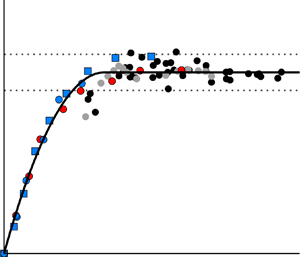
 Figure 8(a), obtained from the cited experimental study of the authors, shows the influence of the Reynolds number on the normalised interaction length for different shock-intensity levels (pressure coefficients  $c_{p}$). Figure 8(b) demonstrates the application of the modified scaling method to all obtained experimental data, indicating a pronounced joint path of the dependence of the normalised interaction length on the normalised interaction strength. The dashed line corresponds to the best-fit approximation of the data and thus represents the desired scaling law for quasi-stationary SWTBLI. The solid lines sorted by the pressure coefficient (shock intensity) in figure 8(a) represent the paths of interaction length versus Reynolds number reconstructed using this scaling law.

Figure 8. Mach 3 experiment results from Touré & Schülein (Reference Touré and Schülein2020): (a) Reynolds number influence on the scaled interaction length; (b) modified scaling approach (2.1) and (2.2) considering the Reynolds number impact on the interaction length.
The reference scaling law for steady interacting flows was needed to analyse the impact of travelling impinging shocks on the non-dimensional interaction length. To achieve steady-state flow with respect to the travelling shock wave, an originally stationary SWTBLI was brought to an almost constant travelling speed relative to the stationary plate model in the wind tunnel experiment. Due to the expected technical problems, wind tunnel tests could only be successfully carried out in a limited range of shock-front speeds (up to approximately  $90\ {\rm m}\ {\rm s}^{-1}$ or 15 % of free-stream velocity). Nevertheless, the data obtained were reproducible and quantitatively valuable. Although the measured interaction length $L$ of the travelling SWTBLI was smaller than that of the stationary interaction in all cases, the scaled results were in each case within the scattering range of the stationary scaling law as soon as the true shock wave Mach number of $M_{s}=(U_\infty +U_{trav})/a_\infty$ was taken into account (figure 9). The reduction in the absolute interaction length could thus be attributed to the thinning of the boundary layer with a decreasing $x$ coordinate and, on the other hand, to the effectively higher Mach number. No other effects of the shock-front movement could be shown.

Figure 9. Experimental results from Touré & Schülein (Reference Touré and Schülein2020) showing that at  $M_\infty = 3$, the shock-front motion with $M_{trav} \approx 0.5$ has no influence on the normalised interaction length.
In the technically limited range of the shock-front speeds, it was simply not possible to determine and exceed the limit of the assumption for a steady flow of the modified scaling law. Therefore, it remains unclear above which shock-front speed this law may no longer be applied to predict the interaction length. Additionally, the role of the originally existing separation bubble in the resulting topology of the travelling SWTBLI (possible historical effects) could not be experimentally clarified. For this reason, the current study was conducted using numerical simulations.
3. Numerical approach
The CFD simulations in this study are carried out with the DLR-TAU code (Schwamborn et al. Reference Schwamborn, Gardner, von Geyr, Krumbein, Lüdeke and Strümer2008). The applied method is described as follows. To validate the code, seven steady, three-dimensional (3-D) RANS simulations corresponding to experimental test cases are carried out. To investigate the effect of shock-travelling speed, 14 simplified, steady, two-dimensional (2-D) RANS simulations serve as references for 2-D unsteady simulations, with varying impinging shock strengths and varying isothermal wall temperatures. Three of those 2-D steady set-ups are utilised for unsteady simulations to investigate the effect of the shock travelling speed for high and low impinging shock strengths and high and low isothermal wall temperatures. All cases with their parameters and results are listed in tables 5, 6 and 8 in the results section. Three-dimensional unsteady simulations were not feasible due to the necessary computation times being approximately 3.2 mio CPUh per investigated shock travelling speed. This high number results from the physical time steps needed of  $O(10\ {\rm ns})$ combined with a high number of inner iterations per physical time step of $O(100)$ and a large domain size needed for one to reach large travelling distances for a completely transitioned, fully uniform SWTBLI movement from an initial stationary state.
The DLR-TAU code uses a 3-D compressible finite-volume method with hybrid grids. A backwards Euler relaxation solver is utilised for fully turbulent simulations, in which the RANS equations are closed by the shear stress transport model by Menter, Kuntz & Langtry (Reference Menter, Kuntz and Langtry2003) (Menter-SST). Simulations using the explicit algebraic Reynolds stress model of Rung et al. (Reference Rung, Lübcke, Franke, Xue, Thiele and Fu1999) (EARSM) were conducted for turbulence model comparisons (Touré Reference Touré2022). The inviscid fluxes are solved by using a second-order upwind method with a flux splitting scheme (AUSMDV; Wada & Liou Reference Wada and Liou1994).
3.1. Grid refinement study for steady 3-D simulations
The simplified 3-D CFD set-up is shown in figure 10 with domain sizes of  $L_x=770$ mm, $L_y=500$ mm and $L_z=250$ mm. As boundary conditions, a supersonic inlet and supersonic outlet are selected. The wind tunnel walls are modelled as Euler walls, and all model surfaces are modelled as viscous walls. To save computational costs, only a half-model with a symmetry plane at $z=0\ {\rm mm}$ is used, and the span of the flat-plate model is assumed to be simplified over the entire width of the test section (full span). A structured grid is utilised for the boundary layer areas of the flat plate and part-span shock generator with a width of 122.5 mm (half-model). For the outer flow field, an unstructured grid is used. For simulations with SWTBLI, the wider shock area in the outer flow field was additionally manually refined.

Figure 10. Sketch of the simulated CAD half-model ( $x$–
$x$– $y$ symmetry plane), with a full-span plate and part-span shock generator.
The grid changes applied for the grid refinement study are shown in table 2. The total grid point number of the analysed grid (Grid 1) is  $38.8 \times 10^6$. The grid influence on the solution is analysed by varying the minimum grid spacing in the plate boundary layer region in the wall-normal direction from $y^+ < 1$ (Grid 2) to $y^+ < 0.1$ (Grid 1). For Grid 3, the outer flow field resolution was automatically doubled by the TAU-Code adaptation module in the regions with high computed density, velocity, total enthalpy or total pressure gradients. This step results mainly in a higher grid resolution of the impinging shock front, which lies within the manually refined area. Furthermore, the structured grid resolution was alternatively doubled in the $x$-axis direction (in a large area around the interaction region) for Grid 4 and in the $z$-axis direction for Grid 5.
Table 2. Grid set-ups for the grid refinement study.

The results of the grid refinement study are shown in figure 11 with the corresponding discrepancy values listed in table 3. The normalised discrepancies for each individual flow parameter were uniformly calculated according to the scheme  $\Delta X \equiv ( X_{fine} - X_{initial\ grid} ) /X_{initial\ grid}$. Here, $X$ represents each examined parameter ( $\,p_{max}$, $\dot {q}_{max}$ or $L_{sep}$). Figure 11(a) shows the dimensionless first-cell-distance distribution $y^+(x)$ for Grids 1 and 2. A tenfold increase in the minimum spacing compared with the fine mesh results in only minor savings in the total grid point number. Nevertheless, the pressure distributions in figure 11(b) and the heat-flux distributions in figure 11(c) are similar for both grids. The largest difference between the solutions for Grid 1 and Grid 2 occurs in the prediction of the separation length $L_{sep}$ ( $\Delta L_{sep} = -4.5\,\%$). Separation and reattachment points were determined in each case as usual from the skin-friction distributions (figure 11d). All other mesh refinements have only minor effects on the separation length, as shown in table 3. Only the difference in the maximum heat-flux density is noticeable with $\Delta \dot {q}_{max} = 3.3\,\%$ for Grid 5.

Figure 11. Grid refinement results for steady 3-D simulations with  $T_{w} / T_{r} = 1.2$: (a) dimensionless wall distance $y^+$, (b) mean wall pressure $p$, (c) heat-flux density $\dot {q}$ and (d) skin-friction coefficient $c_f$.
Table 3. Discrepancy values of the grid refinement study, always relative to Grid 1.

3.2. Time-convergence study for unsteady 2-D simulations
To save computing resources, most of the numerical simulations have been performed on 2-D grids, which corresponds to the simplified view of an infinitely wide test model. Although in the present work unsteady SWTBLI simulations were carried out for both cooled walls and heated walls, the influence of the physical time step size  $\Delta t$ is analysed here only for the cooled wall case. The numerical flow simulation with a cooled wall nominally requires a higher spatial resolution near the wall (smaller first-cell distance) and is thus more sensitive in terms of the required number of iterations.
The starting condition of the unsteady simulation was the stationary separated SWTBLI solution. Since at high shock-front speeds  $U_{trav}$ the jump in the conditions from the quasi-stationary simulation ( $U_{trav} = 0$) to the simulation with a running shock front would be too great, the speed had to be successively increased. During this transient phase, the target speed of the shock front was reached in steps of $50\ {\rm m}\ {\rm s}^{-1}$, with each individual speed jump being followed by a short settling phase of 25 time steps. The maximum distance travelled during the transient phase was approximately 4.3 mm for $U_{trav} = 450\ {\rm m}\ {\rm s}^{-1}$. Since the simulations with a moving shock generator each start from a stationary solution, the distance between the initial position and final position of the shock generator was used to achieve a steady movement of the shock-impingement position and a stationary contour of the shock front. Even at the highest shock-front speed, the duration of the transient phase was less than 2 % of the total simulated test time.
For the time convergence study, the test case with a shock front speed of  $U_{trav} =\Delta x_{\Delta t} / \Delta t =300\ {\rm m}\ {\rm s}^{-1}$ was chosen. Table 4 shows the four physical time steps $\Delta t$ investigated in this study as well as the path distances $\Delta x_{\Delta t}$, which correspond to each time step. In each case, the number of inner iterations per time step was set to 600. In figure 12, the influence of the time-step sizes on the simultaneous distributions of the unsteady wall pressure, heat-flux density and skin-friction coefficient along the flat plate is shown.
Table 4. Investigated physical time step sizes.

Figure 12. Convergence of the solutions with a reduction in the time step  $\Delta t$ for a 2-D SWTBLI travelling with $U_{trav} = 300\ {\rm m}\ {\rm s}^{-1}$ at $T_{w}/T_{r} = 0.4$: (a) mean wall pressure, (b) heat-flux density and (c) skin-friction coefficient.
Particularly striking is the instantaneous pressure distribution for the coarsest time step of 120 ns, which shows a large-scale ripple far downstream of the interaction region that quickly disappears at finer time steps. Similar patterns are visible in the distributions of the heat-flux density and skin-friction coefficient. At finer time steps, a convergence of the results for all three parameters to the solutions of the two finest time steps is visible. In conclusion, for the investigated shock-front speed of  $300\ {\rm m}\ {\rm s}^{-1}$, the time-step size of 40 ns and the corresponding path distance $\Delta x_{\Delta t}$ of $12\ \mathrm {\mu }{\rm m}$ proved to be sufficient. To obtain a guideline for the required time-step size at other shock-front speeds, the value $\Delta x_{\Delta t} = 12\ \mathrm {\mu }{\rm m}$ was kept constant in the main study.
4. Results and discussion
4.1. Validation of CFD simulations
4.1.1. Topology of quasi-stationary interacting flow
The 3-D RANS simulations, comprising seven individual test cases listed in table 5, were carried out to produce a numerical reference dataset as accurately as possible. A validation of these simulations against the experimental data from Touré & Schülein (Reference Touré and Schülein2020) is aimed at identifying possible uncertainties that can be taken into account in the analysis of the simplified 2-D simulations. The numbering of the test cases (first column) was performed according to the interaction strength. The nominal shock intensity  $\xi _{imp} = p_2/p_1$ is defined as the inviscid pressure ratio that is expected locally at the virtual impingement location in the absence of the flat plate. The test matrix of 2-D RANS simulations performed under steady flow conditions is shown for comparison in table 6. In this case, two separate sets of simulations were performed (B and C) to better illuminate the influence of the wall temperature ratio on the steady-state SWTBLI. The stationary interaction datasets that were investigated contain a variation in $\xi _{imp}$ between 1.82 and 3.81.
Table 5. Test matrix and results of steady 3-D RANS simulations.

Table 6. Test matrix and results of steady 2-D RANS simulations.

Figure 13 shows example shadowgrams for test case A3 that were experimentally obtained (figure 13a) and numerically predicted (figure 13b). The numerical and experimental images show qualitative agreement. The interaction of the impinging shock (IS) with the incoming boundary layer (BL) leads to the formation of a separation bubble. The separation bubble itself is normally not directly visible in shadowgrams. However, its existence can be indirectly detected by means of two isolated shock waves (SS and RS), which are typical for separated flows. The separation shock (SS) occurs near the separation zone and physically corresponds to the reflected shock. The recompression shock (RS) occurs behind the recirculation zone and is perceived as a compression fan that transforms into a shock with increasing distance from the wall.

Figure 13. Experimentally obtained (a) and numerically predicted (b) shadowgrams for test case A3.
The numerically predicted surface pressure distribution on the flat plate in this case is shown in figure 14. Upstream of the interaction region, the simulation adequately reproduces the undisturbed turbulent boundary layer. The arc-shaped path of the upstream-influence line suggests a three-dimensionality of the interacting flow, which is attributed to the finite span of the shock generator of 245 mm. Downstream of the interaction area, an additional reflection of the impinging shock on the sidewalls of the wind tunnel ( $z = \pm 0.25$ m) is visible, which could not have any influence on the flow in the investigated area along the centre line.

Figure 14. Pressure coefficient distribution on the flat-plate surface predicted for test case A3, with a shock generator spanwise length of 245 mm (solution mirrored on the symmetry plane).
Figure 15(a) shows a detailed view of figure 14 in the area of the separation bubble with superimposed skin-friction lines. The numerically predicted streamline topology was verified by corresponding skin-friction-line patterns obtained in wind tunnel tests using the oil film interferometry technique (Schülein Reference Schülein2006) and shown in figure 15(b). In agreement, both skin-friction-line patterns show a gently curved shape of the separation line  $S$, while the reattachment line $R$ runs almost linearly and parallel to the $z$ axis. The visualised and predicted skin-friction lines show that outside the symmetry axis, there is basically a transverse secondary flow component, each pointing outwards from the symmetry axis and increasing with distance from it. When this mass flow component in the $z$ direction of the nominal 2-D flow is taken into account, as in the experiments or the 3-D simulations, the flow is defined as 3-D in the context of this work. According to critical-point theory, it is therefore expected that there are at least two singular (critical) points on the symmetry axis, a separation saddle point $S_1$ and an attachment node point $R_1$, from which the corresponding separation and reattachment lines originate (see e.g. § 2 of Babinsky & Harvey (Reference Babinsky and Harvey2011)). The separation lengths between points $S$ and $R$ slightly differ due to an overestimation in the simulation. The determined flow topology is plausible and was expected due to the finite span of the shock generators. However, this finding should not call into question the validity of the results, which are consistent in themselves but should only be taken into account accordingly in the data analysis.

Figure 15. Visualisation of the wall streamline topology on the plate to illustrate the lateral flow component inside the separation bubble for test case A3: numerical wall streamlines (a) and experimental skin-friction lines detected using the oil film interferometry technique (b).
A quantitative comparison of the interaction length between the simulation and the experiment is possible, for example, by using the pressure distributions along the centre line of the flat plate. Figure 16 shows the numerical and experimental pressure distributions for test cases A3 ( $\xi _{imp} = 2.557$) and A6 ( $\xi _{imp} = 3.584$) listed in table 5. At first glance, the results show relative agreement, but they also reveal some problem areas that vary by test case. If in the first case the prediction of the maximum wall pressure behind the separation bubble is satisfactory, in the second case, this value is obviously slightly underestimated. Discrepancies in the location of the upstream impact point indicate in both cases a systematic overestimation of the interaction length, which can be given as $\Delta L = 10\,\%$ (2.8 mm) and $\Delta L = 6\,\%$ (3.1 mm). Considering all seven test cases from table 5, the predicted interaction length overestimates the experiment by 7.5 % on average. Although this result seems to be an acceptable accuracy for RANS modelling (cf. Brown Reference Brown2013), in the current study, we need a higher degree of confidence that the numerical simulations are trustworthy. For this reason, in the next section, we perform a targeted and comprehensive validation of the numerical simulations using an improved empirical scaling law for the interaction length.

Figure 16. Wall pressure distributions along the axis of experimentally measured symmetry and numerically simulated symmetry for test cases A3 ( $\xi _{imp} = 2.557$) and A6 ( $\xi _{imp} = 3.584$).
4.1.2. Validation by enhanced scaling approach for interaction length
The need to further develop the scaling approach of Touré & Schülein (Reference Touré and Schülein2020) arose from the idea of validating all simulation data of the current study with the collection of empirical data used in the cited work. The existing scaling approach, as explained in § 2.1, does not take into account the influence of the wall temperature effect on the interaction length, which has an important role in the current study. This disregard in the existing scaling is demonstrated in figure 17(a), where a distinct stacking of the path according to the wall temperature ratio is observed using the experimental data of Jaunet et al. (Reference Jaunet, Debiève and Dupont2014). Varying the shock strengths at a Mach number of 2.3 and a Reynolds number of  $Re_{\delta } = 0.58 \times 10^5$, two different wall temperature ratios were investigated in this work with $T_{w} / T_{r} = 1$ (adiabatic wall) and $T_{w} / T_{r} = 1.9$ (heated wall).

Figure 17. Interaction-strength scaling for two datasets from Jaunet et al. (Reference Jaunet, Debiève and Dupont2014): (a) without wall temperature correction (equation (2.1)); (b) with the new correction for the wall temperature effect (equation (4.1)).
Jaunet et al. (Reference Jaunet, Debiève and Dupont2014) had tried to extend the scaling approach of Souverein et al. (Reference Souverein, Bakker and Dupont2013) by the wall temperature effect by adding the skin-friction coefficient of the undisturbed flow  $c_{f}$ to the scaling function. This approach was justified with reference to the classical free-interaction theory (Chapman, Kuehn & Larson Reference Chapman, Kuehn and Larson1958). Although the scaling method adapted in this way gave good results for the validation cases and could later be extended to variable Mach numbers by Volpiani et al. (Reference Volpiani, Bernardini and Larsson2020), it unfortunately proved unsuitable for Reynolds numbers $Re_{\delta } > 10^5$. The reason for this outcome is the free-interaction theory itself, which only considers the viscous forces in balance with the pressure gradient, so that a decrease in the skin-friction coefficient with increasing $Re_{\delta }$ automatically increases the interaction length. However, this finding is demonstrably true only for laminar and low-Reynolds-number turbulent flows (see e.g. Babinsky & Harvey Reference Babinsky and Harvey2011, pp. 55, 61). As the Reynolds number is further increased, the momentum of the near-wall turbulent flow gradually takes over the dominant role in SWTBLI zones. Any attempt to explain the complex influence of the Reynolds number on the interaction length in relevant turbulent flows on the basis of skin-friction variations alone is still condemned to failure.
In the present work, an independent attempt has been made to account for the wall temperature effect within the described scaling approach of Touré & Schülein (Reference Touré and Schülein2020). For simplification, similar to the scaling factor  $K_1 = f(Re_{\delta }, c_{p})$ in (2.1), an additional scaling factor $K_{2} = f(T_{w} / T_{r}) = (T_{w} / T_{r})^n$ is introduced, which directly depends on the temperature ratio and includes only one free parameter $n$ for fitting. Using the best-fit approximation performed on the available empirical data listed in table 7, the value for the exponent was determined to be $n = 0.15$. Although the Reynolds numbers $Re_{\delta }$ in the dataset of Jaunet et al. (Reference Jaunet, Debiève and Dupont2014), which maps the effect of wall temperature, were slightly smaller than the discussed limit of $10^5$, this uncertainty had to be accepted due to the lack of well-documented alternatives. The new normalisation of the interaction strength is
 \begin{equation} c_{p}^*= K_{1}K_{2}c_{p} = \left( \frac{Re_{\delta}}{2\times 10^5}\right) ^{-0.27 c_{p}^{1.41}}\left( \frac{T_{w}}{T_{r}}\right)^{0.15}c_{p} . \end{equation}
Figure 17(b) again shows the data from Jaunet et al. (Reference Jaunet, Debiève and Dupont2014) to demonstrate the effect of this new wall temperature correction. Building on this, figure 18 shows the effect of the proposed temperature compensation in determining the interaction strength using all the data listed in table 7. It is evident that the temperature compensation has also purposefully led to further consolidation of the data (figure 18b), which previously showed a distinct layering by wall temperature ratio (figure 18a). Another point stands out when analysing data in figure 18(b). By comparing the results of 2-D simulations (green crosses, tabulated in table 6) with the experimental results (black dots), the influence of the slenderness level of the shock generator on the scaled interaction length  $L^*$ becomes visible. With increasing interaction strength, the scaled interaction length grows faster in the 2-D simulations than in the experiment, leading to increasingly divergent trends. This finding is plausible and attributed to the different topology of the separation bubbles in the 2-D and 3-D cases, as previously discussed. The slight deviations in the $L^*$ values in the 3-D CFD simulations from the experiment are attributed to a general overprediction of the interaction length in the RANS simulations, as discussed in § 4.1.1. However, the agreement of the data over a wide range of interaction strengths is consistent with expectations and considered a validation of the RANS code applied.

Table 7. Data collection considered in figure 18.
 $^{{a}}$Delft University of Technology. $^{{b}}$Institut Universitaire des Systémes Thermiques Industriels, Marseille. $^{{c}}$Chinese Academy of Sciences. $^{{d}}$University of Maryland. $^{{e}}$German Aerospace Center, Göttingen.
A correlation as accurate as possible describing the scaling law obtained for quasi-stationary 2-D flows is needed as a reference for the actual investigation of a moving 2-D SWTBLI. For this reason, two separate scaling laws are defined here: a scaling law for 2-D reference flows and a scaling law for more realistic (3-D) flows near shock generators with moderate slenderness ratios. The best approximation to the empirical correlation for the scaled interaction length, based on the literature data and present 2-D simulations, is described by the following polynomial (coefficient of determination  $R^2$ of 0.99):
 \begin{equation} L^* = 15.46 (c_{p}^*)^2 - 1.07 (c_{p}^*)^4 . \end{equation}
The best-fit approximation of the 3-D reference data considering the temperature ratio  $T_w/T_r=1.2$ is (with $R^2$ of 0.99)
 \begin{equation} L^* = 13.56 (c_{p}^*)^2 - 1.54 (c_{p}^*)^4 . \end{equation}
In summary, the established scaling law for 2-D steady simulations with cooled or heated walls (4.1) can serve as a reference to analyse travelling, 2-D SWTBLI in the subsequent part of this work.
4.1.3. Validation by new scaling approach for plateau pressure
The comparison of the pressure distributions in figure 16 also shows another problem of RANS modelling, which pertains to the insufficient prediction of the wall pressure level within the recirculation zone and is well known (see e.g. Brown Reference Brown2013). The qualitative path of the wall pressure along the interaction area, on the other hand, is well reproduced. This path includes, in particular, the formation of the characteristic pressure plateau on the wall, which is particularly striking in the case of extended separation bubbles. When the separation length is reduced, this plateau area shrinks accordingly until it can only be perceived as a kink in the pressure distribution. Due to this feature, the plateau pressure  $p_{p}$ over wide ranges of interaction strengths can be easily determined from the pressure distribution. The pressure ratio $p_{p}/p_1$ also characterises the cumulative separation-shock intensity and is an excellent comparison parameter for validation purposes.
Unfortunately, there is no generally valid empirical correlation that can be considered for the prediction of the plateau-pressure level completely independent of the Mach number, Reynolds number and shock-wave intensity in flows with SWTBLI. In turbulent flows at low and moderate Reynolds numbers, the correlation based on the free-interaction theory (Chapman et al. Reference Chapman, Kuehn and Larson1958) is often applied, which is well tested and at least takes into account the effects of the Mach and Reynolds numbers:
 \begin{equation} p_{p}/p_1 = 1 + 3 \gamma M_1^2 \sqrt{ \frac{2 c_{f,1}}{(M_1^2 - 1)^{0.5}}}. \end{equation}
For higher Reynolds numbers of interest ( $Re_{\delta } > 10^5$), where the classical free-interaction theory is not applicable (see discussion in § 4.1.2), some alternative correlations are known that explicitly map the mentioned pressure ratio as a function of Mach number only. The best known of these correlations was proposed by Zukoski (Reference Zukoski1967):
 \begin{equation} p_{p}/p_1 = 1 + 0.5 M_1. \end{equation}
None of these correlations includes the effect of interaction strength as the predicted plateau-pressure ratio is defined only as an asymptotically accessible maximum value, which can be expected accordingly for extended separation bubbles. Such a definition of the characteristic pressure ratio makes using the correlations for the validation of numerical simulations at low and moderate shock intensities almost impossible.
Inspired by the success of the scaling law for the normalised interaction length, an attempt was made here to represent the normalised plateau pressure as a function of the previously introduced normalised interaction strength  $c_{p}^*$ according to (4.1). The algorithm for determining the plateau pressure in individual test cases is presented in figure 19(a), where a series of pressure distributions from the current numerical study is shown. The values of the plateau pressure were determined either at the kink point of the pressure distribution (for small-scale separation) or at the local maximum of the pressure distribution within the recirculation zone (for large-scale separation). The dimensionless interaction strengths $c_{p}^*$ are listed in the figure and can be applied to obtain further details on the test cases from table 6. A systematic increase in the plateau pressure level with increasing interaction strength is visible in these numerical data.

Figure 19. New scaling approach for plateau pressure in flows with SWTBLI and validation of numerical simulations. (a) Plateau-pressure ratio determined for a numerical dataset listed in table 6. (b) Scaled plateau pressure as a function of the scaled interaction strength.
Figure 19(b) demonstrates the sought dependence of the scaled plateau pressure on the scaled interaction strength using the obtained and available data. To compensate for the influence of the Mach number on the plateau pressure, the normalised plateau pressure increase  $(\,p_{p}-p_1)/p_1$ was additionally scaled by the empirical factor $0.5 M_1$ of Zukoski (see (4.5)). Both the experimental results (blue dots) and numerical results (triangles) of the current study show a common and distinct correlation between the scaled plateau pressure and the scaled interaction strength. Additionally, particularly valuable are the data from an earlier numerical study (Schülein, Schnepf & Weiss Reference Schülein, Schnepf and Weiss2021) (crosses) in a wide Mach number range of $M_1 = 2\unicode{x2013}5$, which impressively confirm the empirical correlation. The scatter of the data is relatively low, especially when distinguishing between 2-D simulations and 3-D simulations. As expected, the numerical data of the 2-D simulations are somewhat higher than those of the 3-D simulations, which is particularly noticeable with increasing interaction strength. Validation of the 3-D simulations using the experimental data confirms a slight systematic underprediction of the plateau pressure level, which is particularly noticeable for weaker interactions. At higher interaction strengths, the scaled numerical and experimental data rapidly approach a value of 1; thus, the original correlation in (4.5) sufficiently describes the data.
The best-fit approximation of the entire reference data yielded a scaling law for the plateau pressure that maps the influences of Mach number, Reynolds number, wall temperature ratio and interaction strength. The derived correlation equation is converted into a generalised form of the Zukoski formula:
 \begin{equation} p_{p}/p_1 = 1 + 0.5 M_1 \tanh(1.7 c_{p}^*), \end{equation}
with the proposed extension of the original correlation appearing as an additional factor  $\tanh (1.7 c_{p}^*)$. The empirical scaling law found should continue to be tested or specified using independent experimental data to serve as a reliable basis for validating numerical simulations in the future.
4.2. Effect of the shock-travelling speed on the SWTBLI
In this section, unsteady 2-D numerical simulations are used to analyse the transition from an initially steady SWTBLI case with a recirculation bubble to an interaction case with a uniformly travelling shock wave. Based on the numerical results obtained, a new semiempirical scaling approach to describe the interaction length of a uniformly moving SWTBLI could be developed, which allows a simplified prediction of the flow topology and interaction length in such flows. This approach is presented at the end of this section.
Table 8 contains all investigated test conditions based on three test cases (B3, B7 and C3). These three cases with different starting conditions are chosen as they highlight the effect of the wall temperature ratio on the travelling SWTBLI (cases B for cooled wall and cases C for slightly heated wall) and, on the other hand, the effect of the impinging shock strength (case B7 corresponds to a stronger SWTBLI than in case B3). The designation of the underlying test cases corresponds to table 6, where the missing reference values for the respective quasi-stationary interaction ( $U_{trav} = 0\ {\rm m}\ {\rm s}^{-1}$) are also obtained. In each individual test case, the shock-travelling speed was increased step by step until the induced separation bubble could no longer be detected. For each pair of analysed test cases, either the diameter of the shock generator or the wall temperature ratio are different. All parameters in table 8 with a subscript ‘ $s$’ correspond to the condition associated with the uniformly moving coordinate system of the shock-front impingement at $x_{imp,s}=291.6 \pm 1.2\ {\rm mm}$. As described in § 3.2, the final uniformly moving impinging shock for each analysed shock-travelling speed is simulated starting from a fully developed steady SWTBLI following a short transient phase.
Table 8. Test matrix and results of unsteady 2-D RANS simulations.

For a better understanding of the effects of the uniform shock-front motion, figure 20 shows the flow topology as sound-velocity distributions for different shock-travelling speeds  $U_{trav}$ using the example of test case B3. Figure 21 illustrates the corresponding quantitative effect of $U_{trav}$ on the separation-bubble length using the skin-friction distributions along the longitudinal coordinate. Test case B3 examined the shock generator configuration with a moderate diameter $d$ of 16 mm, which maintained an axial distance from the plate surface $\Delta y$ of 80 mm during movement. The wall temperature was also kept constant in each case with $T_w$ = 96 K, so that in individual simulations, the ratio of wall to recovery temperature $T_{w}/T_{r, s}$ slightly varied depending on the shock-travelling speed. The variations in all other parameters that are dependent on the shock-travelling speed are obtained from table 8.

Figure 20. Speed of sound distributions for test case B3 (table 8) at various shock-travelling speeds  $U_{trav}$ of $50\ {\rm m}\ {\rm s}^{-1}$ (a), $100\ {\rm m}\ {\rm s}^{-1}$ (b), $150\ {\rm m}\ {\rm s}^{-1}$ (c), $200\ {\rm m}\ {\rm s}^{-1}$ (d), $250\ {\rm m}\ {\rm s}^{-1}$ (e) and $300\ {\rm m}\ {\rm s}^{-1}$ (f). Shock impingement position at $x_{imp,s}=291.05 \pm 0.35\ {\rm mm}$.

Figure 21. Effect of the uniform shock-travelling speed on the skin-friction coefficient of separated SWTBLI (test case B3). Shock impingement position at  $x_{imp,s}=291.05 \pm 0.35\ {\rm mm}$.
With an increase in  $U_{trav}$, two distinct trends are visible: first, a decrease in the size of the separation bubble; and, second, an increase in the speed of sound in the interaction zone. The first trend is illustrated by figure 21, in which the two zero crossings of each $c_f$ distribution move closer together as $U_{trav}$ increases. To quantify the second trend, the temperature ratio between the maximum temperature within the separation bubble $T_{max,bubble}$ and the constant wall temperature $T_w$ of 96 K is shown in figure 22. This temperature ratio increases to the maximum value of 2.96 at $U_{trav}=250\ {\rm m}\ {\rm s}^{-1}$ and then reverses its trend at approximately $U_{trav}=300\ {\rm m}\ {\rm s}^{-1}$.

Figure 22. Effect of the uniform shock-travelling speed on the normalised maximum temperature inside the bubble (test case B3).
One reason for the temperature rise in the separation bubble is the additional kinetic energy introduced by the moving shock generator, which is perceived as an increase in the recovery temperature  $T_{r,s}$ corresponding to the true Mach number of the travelling shock wave $M_{s} = (U_{trav} + U_\infty ) / a_\infty$:
 \begin{equation} T_{r,s} = T_\infty \left(1+r\frac{\gamma-1}{2} M_{s}^2\right). \end{equation}
The relationship between the induced recovery temperature  $T_{r,s}$ and the maximum temperature in the separation bubble $T_{max,bubble}$ is shown in figure 23 for all test cases investigated. Figure 23(a) shows that an increase in shock-travelling speed (arrow) leads to increases in both $T_{r,S}$ and $T_{max,bubble}$. In contrast, figure 23(b) shows the ratio of the wall temperature to the recovery temperature as a function of the ratio of the maximum static temperature in the separation bubble to the wall temperature. A distinct common linear relationship (solid line) forms among these logarithmic coordinates, describing all available data with an accuracy of ${\pm }3.8\,\%$ using the following equation:
 \begin{equation} T_{max,bubble} / T_{w} = 1.06 \left(T_{w}/T_{r,s}\right)^{-0.77}. \end{equation}
The slight layering of the data by interaction strength (dashed lines) can simply be disregarded as a first approximation. Note that this linear dependence only occurs for separated flows.

Figure 23. Influence of the uniform shock-travelling speed on the induced recovery temperature  $T_{r,s}$ and maximum temperature in the separation bubble $T_{max,bubble}$ in absolute (a) and normalised (b) representation.
To quantitatively assess the influence of the shock-travelling speed on the interaction length, the enhanced scaling approach accounting for the wall temperature effect, e.g. discussed in § 4.1.2, is applied to the current numerical data. Figure 24(a) shows the normalised interaction length as a function of normalised interaction strength for all analysed cases. The true shock-front Mach number  $M_{s}$, the corresponding wall temperature ratio $T_{w}/T_{r,s}$ and the shock wave parameters are employed for scaling in cases with travelling shock fronts. In this way, the influence of the shock-travelling speed can initially only be reduced to the effect of the shock-front Mach number to understand to what extent the quasi-stationary 2-D scaling law is still able to describe the conditions in the travelling 2-D SWTBLI. If one takes the quasi-stationary scaling law (4.2) in the form of the plotted correlation (black line) with an uncertainty measure of $\pm$10 % as a decision aid, this critical shock-travelling speed would fall between 200 and $250\ {\rm m}\ {\rm s}^{-1}$ for cases B7 and C3 and between 50 and $100\ {\rm m}\ {\rm s}^{-1}$ for case B3. For higher $U_{trav}$, the influence of the shock-front movement can no longer be described by considering the shock-front Mach number alone. The small number of points that can be described by the quasi-stationary law in figure 24(a) is somewhat deceptive as all true stationary test cases with $U_{trav} = 0\ {\rm m}\ {\rm s}^{-1}$ (green crosses in figure 18b), which are not listed here, also belong to it. The results of this scaling are additionally included in tables 5 and 6 for steady 3-D and 2-D RANS simulations and in table 8 for unsteady 2-D RANS simulations.

Figure 24. Influence of shock-travelling speed on interaction length using the modified scaling approach (4.1) (a) and considering normalised interaction length as a function of normalised shock-travelling speed (b).
In figure 24(b), the scaled interaction lengths  $L^*$ are additionally normalised in each case with the appropriate reference value predicted by (4.2) at a given interaction strength $c_p^*$. The ratio $L^*/L^*_{ref}$ is plotted against the shock-travelling speed $U_{trav}$ normalised by the maximum speed of sound in the separation bubble $a_{bubble}$. Based on the definition, all selected test cases are expected to have a normalised interaction length close to 1 at the smallest shock-travelling speeds. This condition is true at least for test cases B3 and C3 with weak-to-moderate interaction strengths. The results of the ‘strong-shock’ test case B7, on the other hand, tend towards slightly higher values. This discrepancy shows the limitations of the analogy used to determine the ‘equivalent’ interaction strength by simply considering the true shock-front Mach number $M_{S}$. However, as the normalised shock-travelling speed increases, the data points converge towards $U_{trav}/a_{bubble} \approx 1$, where the interaction length approaches zero. Regardless of the wall temperature or the interaction strength, this condition has been reached, which is shown with the three data points at $L^*=0$. As $a_{bubble}$ increases with $U_{trav}$ (consistent with $T_{max,bubble}$), the conditions at reaching $U_{trav}/a_{bubble} = 1$ are a priori unknown. The critical interaction strength, which in each individual case corresponds to the state $U_{trav}/a_{bubble} = 1$ (or $L^*=0$), is referred to here and in the following as $c_{p,1}^*$.
To understand what exactly causes the end of the ‘quasi-stationary’ phase, the hypothesis of an undercutting of a virtual ‘separation criterion’ is explored. As explained in detail in § 1, studies of 2-D quasi-steady SWTBLI flows have shown that the method of Elfstrom (Reference Elfstrom1972) is good at predicting the critical pressure rise at which ‘macro’ separation occurs. The adaptation of the Elfstrom (Reference Elfstrom1972) criterion, analogous to quasi-stationary 2-D flows, could also allow a prediction for travelling SWTBLI (cf. figure 4). For this purpose, the effective Mach number  $M_{slip}$ is determined from the Mach number profiles of the undisturbed boundary layer, similar to the scheme shown in figure 2. Figure 25(a) shows Mach number profiles in the moving coordinate system ( $M_{s,y}=(U_{y} + U_{trav}) / a_{y}$) for test case B7 at two different shock-travelling speeds of $U_{trav}=50\ {\rm m}\ {\rm s}^{-1}$ and $450\ {\rm m}\ {\rm s}^{-1}$ (black lines). Both profiles consist of five superimposed black profiles each, taken from numerical simulations at five different $x$ positions along the plate ( $x=0.153$ m to 0.393 m in steps of 60 mm). The agreement of the respective profiles in normalised coordinates only confirms the expected self-similarity in undisturbed turbulent flows. The extrapolations of the linear part of the Mach-number profiles are shown as blue lines for all investigated $U_{trav}=50\ {\rm m}\ {\rm s}^{-1}$ to $450\ {\rm m}\ {\rm s}^{-1}$ in $50\ {\rm m}\ {\rm s}^{-1}$ steps. Since the initial profiles of the undisturbed flow are independent of the shock-travelling speed, the slope of the tangents shown remains constant. The increasing shock-travelling speed leads to an increase in the $M_{slip}$ value and thus to an increase in the critical pressure coefficient, which is necessary according to the Elfstrom criterion to maintain a separation bubble. The effect of the wall temperature ratio on the effective Mach number $M_{slip}$ is illustrated in figure 25(b). The extrapolated tangents to the linear parts of the undisturbed Mach number profiles differ in the two test cases shown (B7 and C3) due to the different wall temperature ratios. The fundamentally different shock intensities do not play a role in this consideration.

Figure 25. Influence of the shock-travelling speed  $U_{trav}$ (a) and the wall temperature ratio (b) on the effective Mach number at the wall $M_{slip}$ according to Elfstrom (Reference Elfstrom1972): (a) undisturbed Mach number profiles for case B7 at $U_{trav}=50\ {\rm m}\ {\rm s}^{-1}$ and $450\ {\rm m}\ {\rm s}^{-1}$ (black lines), and $M_{s,y}$-profile tangents at examined $U_{trav}$ (blue lines); (b) $M_{s,y}$-profile tangents for case B7 (blue lines: $U_{trav} =50\ {\rm m}\ {\rm s}^{-1}$ and $450\ {\rm m}\ {\rm s}^{-1}$) and case C3 (red lines: all examined $U_{trav}$).
According to Elfstrom (Reference Elfstrom1972), the threshold  $\xi _{elf}$ is the maximum pressure rise for an inviscid regular shock reflection $\xi _{elf} = p_{elf}/p_1$ and a function of ${M}_{slip}$. Table 9 lists the thresholds for nine shock-travelling speeds for both the cold-wall case (B7) and warm-wall case (C3). To relate the SWTBLI to the threshold, the viscous pressure rise $\xi _{visc} = p_{max}/p_1$ at the plate is employed. The expansion waves induced by the shock generator cylinder significantly reduce the pressure jump at the wall compared with the inviscid result. Accordingly, $\xi _{visc}$ must be determined from the wall pressure distribution at each travelling speed and cannot be easily predicted for this set-up.
Table 9. Thresholds  $\xi _{elf}$ for the pressure jump at the plate, due to the interaction, using the method of Elfstrom (Reference Elfstrom1972) (figure 4) for the undisturbed Mach number profiles from figure 25(b).

Figure 26 shows the scaled interaction lengths normalised by the quasi-stationary reference value  $L^*/L^*_{ref}$ and plotted against the normalised pressure jump of the SWTBLI at the wall $\xi _{visc}/\xi _{elf}$. The quasi-stationary reference correlations $L_{ref}$ are different in the 2-D RANS simulation (4.2) and the experiment (4.3). All three test cases investigated (C3, B3, B7) obviously show a similar trend in this diagram. The scaled interaction length $L^*/L^*_{ref}$ approaches a constant when the normalised value $\xi _{visc}/\xi _{elf}$ is significantly larger than 1. Since for true steady-state SWTBLI flows with $U_{trav} =0\ {\rm m}\ {\rm s}^{-1}$ the limit for $L^*/L^*_{ref}$ is a priori 1, an uncertainty measure of $\pm 10\,\%$ (solid grey lines) is assumed on the basis of steady-state SWTBLI flows from this study (grey dots) and from Touré & Schülein (Reference Touré and Schülein2020) (black dots). Approaching the range with $\xi _{visc}/\xi _{elf} \approx 1.2\unicode{x2013}1.3$, the normalised interaction length $L^*/L^*_{ref}$ starts to decrease. However, for the steady-state cases it is a symptom of greater uncertainty for the weakest interactions measured. Below this range, the trend sharply intensifies. With a further decrease in $\xi _{visc}/\xi _{elf}$ due to the successive increase in the shock-travelling speed $U_{trav}$, the parameter $L^*/L^*_{ref}$ inevitably decreases towards zero.

Figure 26. Normalised interaction length as a function of interaction intensity related to Elfstrom's critical shock reflection intensity.
Using the three depicted trends (C3, B3, B7), a limit for  $\xi _{visc}/\xi _{elf}$ is defined, above which the interaction length is approximately described by the quasi-stationary scaling law, as denoted by the dashed square on the $x$ axis. Due to the existing scatter of the normalised interaction length of approximately $\pm 10\,\%$ (solid grey lines), the corresponding critical range is given as approximately $\xi _{visc}/\xi _{elf}=1.25 \pm 0.05$ (dashed area). The corresponding critical value of the scaled interaction strength $c_{p,2}^*$ depends on the initial quasi-stationary condition. The interaction region is compressed compared with the quasi-stationary case if $c_{p}^*$ is smaller than $c_{p,2}^*$.
The final presentation of the numerical results is shown in figure 27 with the scaled interaction length  $L^*/L^*_{ref}$ plotted against the new scaled interaction strength $\tilde {c}_{p}$ for moving and quasi-stationary SWTBLIs:
 \begin{equation} \tilde{c}_{p} = \left(c_{p}^* - c_{p,1}^*\right) / \left(c_{p,2}^* - c_{p,1}^*\right) . \end{equation}
For the steady-state interactions it is assumed that the equivalent critical interaction strength  $c_{p,1}^*$ should be zero, because they follow the reference scaling laws in figure 18(b). Parameter $c_{p,2}^*$ still corresponds to the situation $\xi _{visc} = 1.25\xi _{elf}$. For this reason, $\tilde {c}_{p} = c_{p}^* / c_{p,2}^*$ applies to these data.

Figure 27. Generalised scaling approach for the simultaneous representation of the normalised interaction length as a function of the normalised interaction strength for stationary and moving 2-D SWTBLIs when increasing the shock-travelling speed from zero to arbitrarily large.
Starting from a quasi-stationary solution at any value greater than 1, the rescaled interaction strengths  $\tilde {c}_{p}$ for cases C3, B3 and B7 steadily decrease with increasing shock-travelling speed. Traversing the $\tilde {c}_{p}$ range between 1 and 0 describes the transition range from a quasi-stationary interaction case with a fully developed (normal-sized) separation bubble to a case in which a separation bubble cannot exist. Accordingly, in the transition region, the normalised interaction length $L^*/L^*_{ref}$ gradually shrinks from 1 to 0. The chosen dimensionless representation reveals a common trend in the range of the shrunken SWTBLI, which can be well described by the following polynomial:
 \begin{equation} L^*/L^*_{ref} =-0.963\,\tilde{c}_{p}^{\,2} + 1.963\,\tilde{c}_{p}. \end{equation}
Thus, the influence of the shock-travelling speed is divided into three groups:
(i) the effect is described by quasi-stationary scaling laws ( $\tilde {c}_{p} > 1$);
(ii) the effect noticeable by the shrunken interaction length (
$0 < \tilde {c}_{p} \leq 1$); and(iii) the absence of upstream influence due to local supersonic speed (
$\tilde {c}_{p} \leq 0$).


The first group covers technically relevant supersonic scenarios, such as travelling shock fronts during ramjet takeoff or angle-of-attack sweep in flight (Liu & Zhang Reference Liu and Zhang2011). The second and third groups are investigated for academic reasons.
The numerical results confirm and explain the experimental results of our own earlier study. The shock-travelling speeds of  $U_{trav}=90\ {\rm m}\ {\rm s}^{-1}$ achieved in that study were simply too low and in the first group under the given inflow conditions to show their influence on the interaction length.
With the knowledge gained from the present work, it is possible to predict by how much the interaction length of a SWTBLI shrinks due to the influence of the shock-travelling speed. In Appendix A, the determined scaling laws are presented in a bundled and application-oriented form for this purpose. This situation also provides an opportunity to test the predictive ability of the scaling approaches on new datasets that were not employed in the development of the approach. The authors are not aware of any comparable study in the literature that has investigated a steady moving SWTBLI that has dynamically evolved from a stationary SWTBLI.
5. Conclusion
Experimental and numerical investigations of separated, quasi-stationary and moving SWTBLIs were performed at a Mach number of 3 and a unit Reynolds number of  $46\times 10^6\ {\rm m}^{-1}$. The main findings of the study are summarised as follows.
(i) New and existing empirical data on quasi-stationary SWTBLI have been thoroughly analysed over a wide range of interaction strengths to identify a scaling approach that allows the prediction of the scaled interaction length and normalised plateau pressure with sufficient accuracy. This success is based on a significant improvement in the scaling approach for the interaction strength known from the literature, which was primarily achieved by a more adequate modelling of the effects of the Reynolds number and wall temperature.
(ii) Two resulting empirical scaling laws for the interaction length and plateau pressure, both as a function of the rescaled interaction strength, were successfully applied to comprehensively validate the results of the 3-D RANS simulations for quasi-stationary SWTBLI cases. The agreement between the experimental and numerical data slightly exceeded expectations based on known comparable validation studies.
(iii) Based on the extensive numerical results of 2-D unsteady RANS simulations for moving SWTBLI, which were validated with the previously obtained experimental data in the limited range of shock-travelling speeds, we discovered that the quasi-stationary SWTBLI corresponds to the maximum possible interaction length at a given interaction strength. An increase in the Mach number of the shock front due to steady upstream motion leads to a decrease in both the scaled interaction length and scaled interaction strength. Three speed ranges with distinctly different properties are identified and described:
(a) At low shock-travelling speeds (range 1), the decrease in interaction length shows quantitative agreement with the prediction of the quasi-stationary scaling law if one corrects the interaction strength according to the shock-front Mach number. The distance between this adjusted interaction strength and the critical strength that would be necessary to basically obtain a recirculation bubble in the boundary layer (Elfstrom criterion) decreases with increasing shock-travelling speed.
(b) As soon as this critical interaction strength is undershot, a new velocity range begins (range 2), in which the dependence of the interaction length on the interaction strength is explicitly influenced by the shock movement. With increasing shock-travelling speed, the scaled interaction length decreases at a significantly faster rate than in the quasi-stationary reference case, which is mainly attributed to the accelerated shift of the sonic line (in the coordinate system of the impinging shock) towards the wall. The end of this velocity range is reached when the subsonic region in the incoming flow completely disappears and the interaction length thus becomes zero.
(c) From this shock-travelling speed onwards (range 3), the impinging shock penetrates the boundary layer up to the wall as the local shock Mach number (local ratio of the absolute shock-front speed to the speed of sound) is greater than 1 everywhere, and shock reflection becomes possible without classical upstream influence. Since the maximum speed of sound cannot be calculated exactly in SWTBLI flows in general and still depends on the shock-travelling speed here, this physical relationship could only be demonstrated by analysing the current numerical results.
(iv) With the knowledge gained, the scaled interaction length can be predicted for both quasi-stationary shock waves and moving shock waves. The identified physical criteria characterising the individual stages of the transformation of the interaction zone by the increase in the shock-travelling speed enabled a targeted and adequate application of the empirical correlations for the prediction of the interaction length.
In the present study, the influence of the shock-travelling speed on the SWTBLI was characterised in detail using a canonical geometry, but some aspects remain unanswered. The realisable shock-front speeds in the experiment were not large enough to validate all numerical findings on the moving SWTBLI, which is therefore still pending. Furthermore, the presented methodology for predicting the interaction length in quasi-stationary and moving SWTBLIs (Appendix A) still needs to be tested with more independent data.
Declaration of interests
The authors report no conflict of interest.
Appendix A
A method to predict the interaction length of a moving SWTBLI is schematically explained for a wedge-shaped shock generator of infinite depth with a deflection angle of the incident flow  $\varphi$, which induces an impinging shock with a constant shock angle up to the impingement point on a flat plate. Starting from a quasi-stationary SWTBLI, the shock generator is accelerated to an arbitrary speed $U_{trav}$. Furthermore, the flow conditions $M_\infty$ and $Re_{\delta }$, as well as the wall temperature $T_{w}$ must be given. The undisturbed boundary-layer velocity profile must also be known or predicted according to the inflow conditions (see e.g. Elfstrom Reference Elfstrom1972).
First, the scaled interaction strength  $c_{p,s}^*$ is determined from the true shock-front Mach number ${M}_{s} = (U_{trav} + U_\infty ) / a_\infty$ and the deflection angle $\varphi$. For this purpose, the resulting inviscid pressure jump $\xi_{s}=p_{out}/p_{in} = p_3/p_1$ as pressure coefficient $c_{p,s}$ as well as the recovery temperature $T_{r,s}$ are calculated and inserted into the corresponding equation (4.1):
 $$\begin{gather} c_{p,s} = \frac{2}{\gamma} \frac{\xi_{s} - 1}{{M}_{s}^2} , \end{gather}$$
 $$\begin{gather}T_{r,s} = T_\infty \left(1+r \frac{\gamma-1}{2} \, {M}_{s}^2\right), \end{gather}$$
 $$\begin{gather}c_{p,s}^*= \left( \frac{Re_{\delta}}{2\times 10^5}\right) ^{-0.27 c_{p,s}^{1.41}} \left( \frac{T_{w}}{T_{r,s}}\right)^{0.15}c_{p,s}. \end{gather}$$
 The limit  $c_{p,1}^*$, which corresponds to the condition $U_{trav} = a_{bubble}$, can only be iteratively determined, e.g. by gradually increasing the sought shock-front Mach number $M_{i}$. At each iteration step, the recovery temperature $T_{r,i}$ and the maximum temperature inside the bubble $T_{i}$ are calculated to determine the maximum induced speed of sound $a_{i}$ and the shock-travelling speed $U_{trav,i}$:
 \begin{equation} \left.\begin{gathered} \mathrm{repeat} \\ \quad M_{i} = M_{i-1} + \Delta M,\\ \quad T_{r,i} = T_\infty \left(1+r \frac{\gamma-1}{2} \, {M}_{i}^2\right),\\ \quad T_{i} = 1.06 \, \left(T_{w}/T_{r,i}\right)^{-0.77} T_w ,\\ \quad a_{i} = \sqrt{\gamma RT_{i}} ,\\ \quad U_{trav,i} = M_{i}a_{i} - U_\infty ,\\ \mathrm{until} \ U_{trav,i} = a_{i}. \end{gathered}\right\}\end{equation}
Using the known flow deflection angle  $\varphi$ and the iteratively obtained Mach number $M_{i}$, the expected pressure jump at inviscid shock reflection $\xi _{i} =p_3/p_1$ can be calculated to determine the critical pressure coefficient $c_{p,1}$ as well as the corresponding critical interaction strength $c_{p,1}^*$:
 $$\begin{gather} c_{p,1} = \frac{2}{\gamma} \frac{\xi_{i} - 1}{M_{i}^2}, \end{gather}$$
 $$\begin{gather}c_{p,1}^* = \left( \frac{Re_{\delta}}{2\times 10^5}\right) ^{-0.27 c_{p,1}^{1.41}}\left( \frac{T_{w}}{T_{r,i}}\right)^{0.15}c_{p,1} . \end{gather}$$
 The limit  $c_{p,2}^*$ can also only be iteratively determined, e.g. by gradually increasing $M_{i}$. This result corresponds to the condition $1.25\,\xi _{elf,i} = \xi _{i}$ respectively $1.25~\xi _{elf,i} = \xi _{visc}$. The inviscid pressure jump $\xi _{i}$ (for $M_{i}$) is applied if expansion waves of a wedge-shaped shock generator induced by the trailing edge have a negligible effect on the interaction zone; otherwise, the viscous pressure jump at the wall must be applied $\xi _{visc}$. To calculate $\xi _{elf,i}$, the effective Mach number at the wall $M_{slip}$ shall be determined in the coordinate system of the moving shock wave from the undisturbed velocity profile and the gradually increasing shock-travelling speed $U_{trav,i}$ corresponding to $M_{i}$ (figure 25). Hence, $\xi _{elf,i} = p_{elf}/p_1$ is a function of $M_{slip}$ and the corresponding maximum deflection angle without shock detachment of the impinging or reflected shock. If the condition is met, the inviscid interaction strength is used to calculate the critical pressure coefficient $c_{p,2}$ as well as the corresponding critical interaction strength $c_{p,2}^*$:
 $$\begin{gather} c_{p,2} = \frac{2}{\gamma} \frac{\xi_{i} - 1}{{M}^2}, \end{gather}$$
 $$\begin{gather}c_{p,2}^*= \left( \frac{Re_{\delta}}{2\times 10^5}\right) ^{-0.27 c_{p,2}^{1.41}} \left( \frac{T_{w}}{T_{r}}\right)^{0.15}c_{p,2} . \end{gather}$$
 From the two critical values  $c_{p,1}^*$ and $c_{p,2}^*$, the normalised interaction strength $\tilde {c}_{p,s}$ can be determined, which is utilized to calculate the scaled interaction length $L^*$:
 $$\begin{gather} \tilde{c}_{p,s} = \left(c_{p,s}^* - c_{p,1}^*\right) / \left(c_{p,2}^* - c_{p,1}^*\right), \end{gather}$$
 $$\begin{gather}L^*_{ref} = 15.46(c_{p,s}^*)^2 - 1.07(c_{p,s}^*)^4, \end{gather}$$
 $$\begin{gather}L^*/L^*_{ref} =-0.963\tilde{c}_{p,s}^{\,2} + 1.963\tilde{c}_{p,s}. \end{gather}$$
Depending on the value of  $\tilde {c}_{p,s}$, there can be three possibilities: (1) for $\tilde {c}_{p,s} \geq 1$, $L^*$ is directly determined from (A10) ( $L^* = L^*_{ref}$); (2) for $0 < \tilde {c}_{p,s} < 1$, $L^*$ is calculated using (A10) and (A11); and (3) for $\tilde {c}_{p,s} \leq 0$, $L^*$ is always zero.
The interaction length  $L$ of the moving SWTBLI is calculated via (2.2), with the shock angle $\beta$ at a given shock-front Mach number ${M}_{s}$ and given $\varphi$:
 \begin{equation} L = L^* \delta^* \frac{\sin(\beta-\varphi)}{\sin\beta\sin\varphi}. \end{equation}


 Open access